

Abstract
In electrocoalescence, an electric field is applied to a dispersion of conducting water droplets in a poorly conducting oil to force the droplets to merge in the direction of the field. Electrocoalescence is used in petroleum refining to separate water from crude oil and in droplet-based microfluidics to combine droplets of water in oil and to break emulsions. Using a microfluidic design to generate a two-dimensional (2D) emulsion, we demonstrate that electrocoalescence in an opaque crude oil can be visualized with optical microscopy and studied on an individual droplet basis in a chamber whose height is small enough to make the dispersions two dimensional and transparent. From reconstructions of images of the 2D electrocoalescence, the electrostatic forces driving the droplet merging are calculated in a numerically exact manner and used to predict observed coalescence events. Hence, the direct simulation of the electrocoalescence-driven breakdown of 2D emulsions in microfluidic devices can be envisioned.
1. Introduction
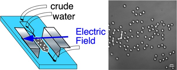
Electric field-mediated coalescence of conducting water droplets dispersed in a continuous, poorly conducting dielectric oil phase (Figure 1) is a long-standing technology in the petroleum refining industry. This technology has been used to remove emulsion droplets of water in crude oil,1−7 particularly in the context of the desalting operation of electrocoalescers. In this operation, fresh water is first introduced into the crude at the inlet to the electrocoalescer to remove organic salts by transferring into the water phase. The introduction of the water creates an emulsion of the water in oil, which is passed between electrodes. The electric field between the electrodes coalesces the salt-laden droplets in the direction of the field. Successive coalescence events between droplets produce progressively larger droplets that settle under gravity into a bulk water phase that can be easily removed. Generally, these water in crude oil emulsions are strongly stabilized against coalescence by the adsorption onto the water/oil interface of surface-active components from the oil, particularly the alkylated, polyaromatic asphaltenes (for reviews, see Mullins et al.8−10). Asphaltenes adsorb onto the interface to form interfacial layers, which in time age and give rise to highly elastic skins that resist droplet coalescence under typical conditions (for reviews, see refs (11, 12) and the studies13−18). In an electrocoalescer, these highly stabilized droplets are forced to merge at sufficiently high electric field strengths. Despite the importance of the electrocoalescence process in the refining industry, the fundamentals of this phenomenon are still evolving. This is in part due to the difficulty of examination of electrocoalescence in crudes because of the oil opacity. Therefore, many studies thus far substitute oil with a clean, transparent fluid that may not reproduce the crude oil environment, e.g., refs (19−23).
Figure 1.

Induced dipole formation on the surfaces of a pair of spherical conducting aqueous droplets in a poorly conducting oil phase due to an imposed uniform electric field E̅ and the dipole–dipole interaction between the droplets, which creates an interdroplet attractive force.
Microfluidics can enable a direct visualization of electrocoalescence in crudes by generating emulsions in which the droplets are arranged in a single layer with a small depth transparent to optical microscopy, e.g., refs (24, 25). Microfluidics also offers the ability to form emulsions of controlled and uniform size (e.g., through the use of “T” junctions, flow-focusing orifices, and capillary tips).26−29 The first goal of this study is to demonstrate these unique fluid handling and visualization capabilities of microfluidics using crude oil to demonstrate how the electrocoalesence process in crudes can be examined in situ using microfluidics.
More recently, interest in electrocoalesence has focused on lab on chip devices30−40 in which two-dimensional (2D) water-in-oil emulsions are used for chemical or biological assays, extractions, and separations. In this context, electrocoalescence has drawn interest as a means for combining droplets and breaking water-in-oil emulsions to complete the chip operations (see for example41−50). As explained below, the model problem of the electrocoalescence of droplet pairs has been theoretically and experimentally examined as in Figure 1. However, few studies have examined theoretically the dynamics of electrocoalescence of emulsions in which the breakdown process is determined by multiple attractive and repulsive forces exerted on each droplet. This multidroplet process underlies the breakdown of water-in-crude oil emulsions and the combining of droplets and the breakdown of emulsions on lab on-chip processes. The second goal of this study is to obtain theoretical solutions for the electric field in the continuous phase of a microfluidically generated uniform 2D emulsion to predict electrocoalescence forces and coalescence events and to compare these predictions with the experiments.
In this study, we use a microfluidic arrangement to generate a train of water droplets in a continuous crude oil phase in a channel. The train is directed to a wide chamber in which the droplets are arranged in a single layer lubricated from above and below by very thin layers of oil. We term this freely moving, two-dimensional assembly a “2D emulsion”. We apply an electric field along the layer to cause the droplets to merge and the emulsion to breakdown. Numerical configurations of droplet arrangements in this 2D emulsion are reconstructed from images of electrocoalescence experiments in a microfluidic chamber. The electrical forces exerted on the droplets are computed to predict merging events. These predictions coincide with the merging events observed in the experiment, suggesting the breakdown can be simulated and potentially programmed, and this is the second motivation of our study.
We begin with a brief review.
Electrocoalescence of an isolated
pair of droplets of water in a continuous oil under a uniform applied
electric field, Figure 1, has been studied theoretically22,51−68 and experimentally.19−22,62,68−77 The electrohydrodynamic forces, which cause the droplets to merge
in the direction of the field, have been described by the field-induced
charge distribution on the surface of the droplets. For an isolated
spherical water droplet of radius a placed in a uniform
oscillating field (E̅ eiωt where E̅ is the amplitude, t is the time, and ω is
the frequency), mobile ions in the water and possibly oil phases are
conducted in the field direction. In electrocoalesence, the conductivities
and dielectric constants of the droplet phase, σp and εp, are larger than those of the oil continuous
phase, σm and εm. Therefore, free
and bound positive (negative) charges accumulate at the side of the
droplet facing (opposite) to the direction of the electric field.
To leading order, an oscillating electric dipole aligned with the
field,  , is induced as given by78−81
 . Here,
  denotes the real part of the bracketed
expression,
denotes the real part of the bracketed
expression,  is the Clausius Mossotti factor defined
in terms of the complex dielectric constants of the oil and water
phases with
is the Clausius Mossotti factor defined
in terms of the complex dielectric constants of the oil and water
phases with  and
and  , and
εo is the permittivity
of free space. Typically, σp ≫ σm and εp ≫ εm, and
hence,
, and
εo is the permittivity
of free space. Typically, σp ≫ σm and εp ≫ εm, and
hence,  . For
a droplet pair, interaction forces
arise principally because the dipole induced on each of the droplets
falls within the dipole electric field created by its neighbor. For
spherical droplets, the interaction depends on the angle of orientation
of the droplet pair axis with the field, θ, and the edge-to-edge
separation distance, s (Figure 1). If the electric field acting on each droplet
is approximated by the far field dipole field of its neighbor, then
the time average pairwise interaction force along the centerline is19−21,82
. For
a droplet pair, interaction forces
arise principally because the dipole induced on each of the droplets
falls within the dipole electric field created by its neighbor. For
spherical droplets, the interaction depends on the angle of orientation
of the droplet pair axis with the field, θ, and the edge-to-edge
separation distance, s (Figure 1). If the electric field acting on each droplet
is approximated by the far field dipole field of its neighbor, then
the time average pairwise interaction force along the centerline is19−21,82
| 1 |
where E̅RMS, the root mean square of the oscillating
field, is
equal to E̅/√2. The dipole field of
the neighbor and correspondingly the force on the droplet intensify
as the droplets approach one another. When the droplets are aligned
with the field, θ = 0, the force is attractive as dipoles line-up
end-to-end. Whereas, when the droplets are alongside each other, θ
= π/2, the force is repulsive as the dipoles are parallel. Exact
solutions for the interaction force between spherical conductors in
a perfectly insulating dielectric ( ) subject to a uniform electric
field are
obtained by Davis83 using bispherical coordinates.
For θ = 0, the interaction force is written in terms of the
nondimensional function
) subject to a uniform electric
field are
obtained by Davis83 using bispherical coordinates.
For θ = 0, the interaction force is written in terms of the
nondimensional function  , i.e.,
  . The bispherical exact solution
for the
force demonstrates that the dipole approximation is valid for s/a > 1, but the exact solution increases
much more rapidly than the dipole approximation for s/a < 1. For 10–3 < s/a < 10–1, a numerical
fit22 is
. The bispherical exact solution
for the
force demonstrates that the dipole approximation is valid for s/a > 1, but the exact solution increases
much more rapidly than the dipole approximation for s/a < 1. For 10–3 < s/a < 10–1, a numerical
fit22 is  . For θ = 0, the
bispherical solution
shows that the maximum value of the electric field is at the poles
of the droplets facing each other and is given by
. For θ = 0, the
bispherical solution
shows that the maximum value of the electric field is at the poles
of the droplets facing each other and is given by  . This can be approximated as22,59
 for 10–3 < s/a < 10–1.
For a single aqueous droplet in oil subject to a uniform field
(e.g., refs (53, 84−86)), the applied field exerts an electrical normal traction (Maxwell
stress) on the induced free or bound surface charge. This, in turn,
causes the droplets to deform in the field direction as prolate figures,
which adopt conical tips (“Taylor” cones) at higher
field strengths before bursting. This deformation scales as the electrocapillary
number  where γ is the interfacial tension.
For isolated droplet pairs approaching each other due to dipolar attraction
and small Ec ≪ 1, the droplets
remain spherical for s/a > 1.
Assuming
spherical shapes (Ec ≪ 1) and balancing
the dipolar interaction force and viscous resistance with the lubrication
theory for close enough separations (typically inertial forces are
negligible), Eow et al.19 and Chiesa et
al.20,21 compute trajectories starting from large
separation distances s/a > 1
and
up to coalescence. Their results agree well with corresponding experimental
trajectories. More recent studies58,60−62,66,67,77 account for interface deformation and again
map successfully theoretical predictions with experimental results
on the trajectories of droplet pairs driven together by electrocoalescence.
where γ is the interfacial tension.
For isolated droplet pairs approaching each other due to dipolar attraction
and small Ec ≪ 1, the droplets
remain spherical for s/a > 1.
Assuming
spherical shapes (Ec ≪ 1) and balancing
the dipolar interaction force and viscous resistance with the lubrication
theory for close enough separations (typically inertial forces are
negligible), Eow et al.19 and Chiesa et
al.20,21 compute trajectories starting from large
separation distances s/a > 1
and
up to coalescence. Their results agree well with corresponding experimental
trajectories. More recent studies58,60−62,66,67,77 account for interface deformation and again
map successfully theoretical predictions with experimental results
on the trajectories of droplet pairs driven together by electrocoalescence.
The details of the final stages of electrocoalescence as the droplets approach to within a few tenths of a radius of each other and merge are more complicated. The merging process takes place on time scales of tens of milliseconds, which are typically much shorter than the time scale for the approach of droplets. As relatively spherical droplets approach (Ec ≪ 1) one another, the electric field exerted on the facing poles intensifies, and pronounced opposing prolate deformations develop that precede coalescence. These deformations have been examined theoretically by accounting for interface deformation in continuum computational simulations61−66 and molecular dynamics simulations.68
The final stages in the electrocoalescence process have also
been
visualized in small fluidic cells or microfluidic arrangements in
which, in a continuous oil phase, an electric field is applied across
free aqueous droplet pairs along their line of centers70−74 or anchored droplets at a fixed potential difference are arranged
to face one another.75,87−94 The dynamics are visualized over a time interval of hundreds of
milliseconds from an initial separation distance so/a. Three regimes are recognized: (i)
no coalescence due to a large gap distance or a too small field strength,
(ii) coalescence at large enough field strengths, or (iii) partial
coalescence and repulsion at typically larger field strengths than
necessary for coalescence. Coalescence is observed as a liquid bridge
forms between the droplets from their individual prolate deformations.
The liquid bridge then grows in radius to the order of the droplet
radii bringing the droplets together into one fluid mass. In partial
coalescence, the facing droplet interfaces are deformed into cones
that connect to form a narrow bridge that becomes unstable, breaks,
and drives a recoil. In the case of coalescence, which is of interest
here, for anchored droplets at fixed potentials, Atten et al.89 measured the critical potential difference Vcrit at which the droplet faces merge. They
correlated their results as the critical electrical capillary number  as a function of so/a < 1 and find critical capillary numbers
in the range of 0.2–0.4. These values agreed with their numerical
calculations and are in the range of other theoretical calculations
of anchored or suspended droplets in close proximity (so/a < 1), e.g., Latham and Roxburgh,51 Taylor,52 and Atten.59
as a function of so/a < 1 and find critical capillary numbers
in the range of 0.2–0.4. These values agreed with their numerical
calculations and are in the range of other theoretical calculations
of anchored or suspended droplets in close proximity (so/a < 1), e.g., Latham and Roxburgh,51 Taylor,52 and Atten.59
The dynamics of electrocoalescence of
multiple water droplets in
water-in-oil emulsions has only been examined recently by Garstecki
et al.95 They generated a 2D emulsion with
flow focusing of water and hexadecane in a microfluidic cell and observed
electrocoalescence across the emulsion under an AC field. They find
a critical field strength necessary for electrocoalescence, which
decreases with decreasing ω and increasing σp. This suggests that the faster the free charge relaxation in the
water droplet phase (time scale  ) relative to the AC
oscillation (1/ω),
the greater is the charge separation (dipole strength) for an applied
field. This is due to a redistribution of more free charge on the
surface and higher droplet polarization, resulting in a greater dipolar
attraction.
) relative to the AC
oscillation (1/ω),
the greater is the charge separation (dipole strength) for an applied
field. This is due to a redistribution of more free charge on the
surface and higher droplet polarization, resulting in a greater dipolar
attraction.
2. Results and Discussion
2.1. Visualization of Electrocoalesence in Crudes in a Microfluidic Cell
Our microfluidic experiments on the visualization of electrocoalescence of water droplets in an opaque petroleum crude are undertaken in a polydimethylsiloxane (PDMS) transparent cell using flow focusing at an orifice to form water droplets in the crude in a channel as a droplet train and directing the train to a wide chamber in which an AC field is applied to the 2D emulsion, which forms cf. Figure 2. (The fabrication of the cell, the material properties of the crude (including the dynamic oil/water tension), and the details of the applied field and frequency are described in the Experimental Section.) Figure 2 shows the flow-focusing production of the water droplets in oil at the orifice and the 2D emulsion of the droplets in the chamber prior to the application of the field. As is clear from the images, the droplets in the crude (which appears opaque and black in a 10 mL test tube) are readily visualized in the microfluidic cell due to the small thickness of the optical slice (60 μm). The droplets are monodisperse in size with a diameter of 2a = 36–48 μm. The assembled 2D emulsion presents interdroplet distances s, which vary from under one droplet diameter to several diameters. The separation distances are quantified when the droplet configuration is rendered for numerical calculation of the electric field and interdroplet forces. Under most circumstances in the flow-focusing generation of water drops in oil, surfactants are required in the oil phase to reduce the oil/water tension. This is necessary so that the water phase, drawn into a thread in the orifice, breaks into droplets.96 Here, the surface-active molecules native to the crude (e.g., asphaltenes) serve this role, and importantly, electrocoalescence of water droplets in crude can be examined in situ without any additional surfactants. The naturally reduced interfacial tensions of crudes against water (here 28 mN/m, Figure 8 in Experimental Section) allow a large deformability of the interface, ensuring that the water is easily segmented into drops at the flow-focusing orifice.
Figure 2.

Schematic of the microfluidic cell including the arrangement of the flow-focusing orifice to form individual droplets and the chamber in which the droplets assemble into a 2D emulsion and the electric field is applied. Shown also are images of the drop generation at the orifice (the schematic and the frame from the video) and the 2D emulsion in the chamber (the frame from the video). The scale bars are 50 μm.
Figure 3 shows an illustrative sequence of images of electrocoalescence
events in the chamber, over a period of approximately 1/2 s, for a
field strength  = 250 V/mm. The images
are a bird’s
eye view of the 2D emulsion, with the field applied top-to-bottom,
and with the assigned times relative to the moment the field is energized
(the video is available in the Supporting Information.) For the first image shown in the sequence, no coalescence events
have occurred. The sequence in Figure 3 includes droplet pairs coalescing, as well as events
in which groups of three and four droplets coalesce. Also evident
(the lower right-hand side of the figure) is a cascading event where
two droplets merge, and the combined drop merges with a neighbor brought
closer due to the prior electrocoalescence event as also observed
by Garstecki et al.95 The coalescence events
are clearly between droplets close enough so that they are a few tenths
of a radius apart. Typically, coalescing droplets are aligned closely
with the field. For an isolated pair of droplets, the dipole interaction
force predicts an attractive force for 0 < θ < θc where θc is given by 3 cos2 θc – 1 =0, cf. eq (1), and is equal
to 54.8°. For all of the coalescence events in Figure 3, the angle between the field
and the line of centers between the droplet pair falls between 0 and
approximately 55° in agreement with the dipole force approximation.
Droplet pairs with angles larger than approximately 55° do not
coalesce, even at close separation distance. Isolated droplet pairs
that merge follow a common pattern in which they deform toward each
other to create a joining liquid bridge (Figure 3). The faces of each drop, which are opposite
to the bridging thread, remain more spherical as the field has not
intensified on those surfaces away from the region between the drops.
The connecting thread increases in radius until the drops merge and
readopt a spherical configuration. While the coalescence process itself
takes place on a time scale of milliseconds, the equilibration to
a spherical shape takes place on a time scale of hundreds of milliseconds
to 1 s. The triple droplet and quadruple droplet merging evident in
the sequence of Figure 3 appear as simultaneous events between the multiple droplets. In
these cases, connecting liquid threads form between adjoining pairs
to form a merged cylinder that eventually relaxes to a spherical shape.
Qualitatively, over the time frame studied, the coalescence events
appear without noticeable movement of the droplets toward each other.
Critical fields required for the coalescence of droplets a few tenths
of a radius close to one another appear to be reached, and the droplets
coalesce in place.
= 250 V/mm. The images
are a bird’s
eye view of the 2D emulsion, with the field applied top-to-bottom,
and with the assigned times relative to the moment the field is energized
(the video is available in the Supporting Information.) For the first image shown in the sequence, no coalescence events
have occurred. The sequence in Figure 3 includes droplet pairs coalescing, as well as events
in which groups of three and four droplets coalesce. Also evident
(the lower right-hand side of the figure) is a cascading event where
two droplets merge, and the combined drop merges with a neighbor brought
closer due to the prior electrocoalescence event as also observed
by Garstecki et al.95 The coalescence events
are clearly between droplets close enough so that they are a few tenths
of a radius apart. Typically, coalescing droplets are aligned closely
with the field. For an isolated pair of droplets, the dipole interaction
force predicts an attractive force for 0 < θ < θc where θc is given by 3 cos2 θc – 1 =0, cf. eq (1), and is equal
to 54.8°. For all of the coalescence events in Figure 3, the angle between the field
and the line of centers between the droplet pair falls between 0 and
approximately 55° in agreement with the dipole force approximation.
Droplet pairs with angles larger than approximately 55° do not
coalesce, even at close separation distance. Isolated droplet pairs
that merge follow a common pattern in which they deform toward each
other to create a joining liquid bridge (Figure 3). The faces of each drop, which are opposite
to the bridging thread, remain more spherical as the field has not
intensified on those surfaces away from the region between the drops.
The connecting thread increases in radius until the drops merge and
readopt a spherical configuration. While the coalescence process itself
takes place on a time scale of milliseconds, the equilibration to
a spherical shape takes place on a time scale of hundreds of milliseconds
to 1 s. The triple droplet and quadruple droplet merging evident in
the sequence of Figure 3 appear as simultaneous events between the multiple droplets. In
these cases, connecting liquid threads form between adjoining pairs
to form a merged cylinder that eventually relaxes to a spherical shape.
Qualitatively, over the time frame studied, the coalescence events
appear without noticeable movement of the droplets toward each other.
Critical fields required for the coalescence of droplets a few tenths
of a radius close to one another appear to be reached, and the droplets
coalesce in place.
Figure 3.

Image sequence of the electrocoalescence of droplets in
the chamber
at times of 1.94–2.56 s, referenced from the moment (t = 0) the field is energized. In the first configuration,
at 1.94 s, no droplets have yet coalesced. The scale bar is 50 μm.
The field is applied top-to-bottom with  = 250 V/mm.
2.2. Theoretical Calculation of Electric Field in the 2D Emulsion
Figure 3 makes clear that, upon application of the electric
field, the electrocoalescence events in the crude oil can be recognized,
cataloged, and sequenced. We demonstrate that these events can also
be predicted by first computing the electric field distribution in
the emulsion and then evaluating the field at the surfaces of the
droplets to calculate the interdroplet forces and identify pairwise
attractive interactions leading to the merging of droplet pairs. For
a given droplet in the emulsion, the electric field that is experienced
is determined by the imposed far field and by the droplets around
them, and therefore the computation of the field is a mulitibody calculation.
We use COMSOL Multiphysics 4.2 to obtain a numerical finite element
solution for the electric field in the continuous oil phase. We start
with an image captured at the beginning of an experiment in which
the field has been turned on, but no coalescence has occurred (e.g.,
the first image of Figure 3). We render the two-dimensional images, representing the
instantaneous configuration of uncoalesced droplets, into a three-dimensional
(3D) COMSOL computational domain. This is intended to reproduce the
observation chamber and the arrangements of droplets in the chamber.
The droplets are modeled as fluid spheres and positioned in the computational
domain at their exact locations in the image. The locations of the
perimeters of the droplets in the 2D images are obtained by edge detection.
The intensity range of each pixel is 0–255, and the perimeter
is located by identifying the change in pixel intensity from bright
(within the droplets) to dark (the exterior crude oil) along directions
approximately perpendicular to the perimeter. The change occurs over
the order of a few pixels, and the perimeter is demarcated as a set
of points at which the area under the intensity vs pixel position
on either side of a given point (relative to the asymptotic values
on either side) is equal. Using this algorithm, the edge is located
to an error of approximately one-half of a pixel or half a micron.
The points are then fit to a circle with a radius, which is assigned
to the radius of the droplet at that point. The center of the circle
is assigned the center location of the droplet. A sphere is constructed
from that center with the assigned radius and positioned halfway between
the top and bottom of the chamber. The domain height is set equal
to the chamber height  = 60 μm,
and the domain width (
= 60 μm,
and the domain width ( = 1 mm) and length (
 =1 mm section) are set equal to
the width
of the chamber and the length observed in the captured image. The
top and bottom are maintained at a potential difference
=1 mm section) are set equal to
the width
of the chamber and the length observed in the captured image. The
top and bottom are maintained at a potential difference  , which is computed from
the driving potential
difference applied across the electrodes inserted into the PDMS (
, which is computed from
the driving potential
difference applied across the electrodes inserted into the PDMS ( ). Values of the dielectric
constant of
the cured PDMS elastomer (2.0)97 are approximately
equal to the measured dielectric constant of the crude (2.5). Hence,
for the purposes of the calculation of
). Values of the dielectric
constant of
the cured PDMS elastomer (2.0)97 are approximately
equal to the measured dielectric constant of the crude (2.5). Hence,
for the purposes of the calculation of  ,
the PDMS and crude in the chamber are
considered as perfect dielectrics in capacitive series, leading to
,
the PDMS and crude in the chamber are
considered as perfect dielectrics in capacitive series, leading to  , which in the experiments is equal to 250
V/mm. Although the droplets settle downward during their residence
time in the chamber, the approximation that they are at the center
of the chamber for the electrostatic calculation is valid because
the dielectric constants of the PDMS and oil are nearly equal. The
applied potential is 0 V on the bottom, −250 V =
, which in the experiments is equal to 250
V/mm. Although the droplets settle downward during their residence
time in the chamber, the approximation that they are at the center
of the chamber for the electrostatic calculation is valid because
the dielectric constants of the PDMS and oil are nearly equal. The
applied potential is 0 V on the bottom, −250 V =  on the top. This is corresponding
to the
experimental gradient of 250 V/mm with the electric field directed
from top to bottom. As the potentials are fixed, the calculations
are undertaken assuming a static DC field is applied. As we demonstrate
below, the equations and solutions for the electric field are all
quasi-static. Hence from these solutions, to obtain the forces on
the droplets to compare to the AC experiments, the square of the DC
field strength used in the force calculations (
on the top. This is corresponding
to the
experimental gradient of 250 V/mm with the electric field directed
from top to bottom. As the potentials are fixed, the calculations
are undertaken assuming a static DC field is applied. As we demonstrate
below, the equations and solutions for the electric field are all
quasi-static. Hence from these solutions, to obtain the forces on
the droplets to compare to the AC experiments, the square of the DC
field strength used in the force calculations ( ) is replaced
by 1/2 the square of the field,
corresponding to the time average of the 250 V/mm AC field in the
experiments.
) is replaced
by 1/2 the square of the field,
corresponding to the time average of the 250 V/mm AC field in the
experiments.
To calculate the electric field, the crude, a poor
conductor, is modeled as a “leaky dielectric”98 with zero volume charge density. This satisfies
∇2ϕm = 0, where ϕm is the oil electrostatic potential (made dimensionless with  ) and formulated in COMSOL’s
cartesian
coordinate representation of the computational domain. Each of the
) and formulated in COMSOL’s
cartesian
coordinate representation of the computational domain. Each of the  spheres in
the computation domain is modeled
as ohmic conductors in which the volume free charge relaxes quickly
relative to 1/ω (i.e., Ω > 1). Therefore, the potential
field in the spheres is quasi-static and satisfies
spheres in
the computation domain is modeled
as ohmic conductors in which the volume free charge relaxes quickly
relative to 1/ω (i.e., Ω > 1). Therefore, the potential
field in the spheres is quasi-static and satisfies  where ϕp(i) is the nondimensional electrostatic potential within drop i. The boundary conditions on the surface of each of the
spheres are continuity of the electric potential, ϕm = ϕp(i), (
where ϕp(i) is the nondimensional electrostatic potential within drop i. The boundary conditions on the surface of each of the
spheres are continuity of the electric potential, ϕm = ϕp(i), ( ) and the surface charge density conditions,
  (charge balance) and ε*ρs(i) = ni ·{ε*∇ϕm – ∇ϕp(i)}
(Gauss’s law). Here, ni is the unit outward normal to the sphere i and
τ is the time nondimensionalized by 1/ω
and ρs(i) is the surface charge
density on droplet i nondimensionalized by
(charge balance) and ε*ρs(i) = ni ·{ε*∇ϕm – ∇ϕp(i)}
(Gauss’s law). Here, ni is the unit outward normal to the sphere i and
τ is the time nondimensionalized by 1/ω
and ρs(i) is the surface charge
density on droplet i nondimensionalized by  .
.  and
and  are, respectively,
the ratios of the conductivities
and dielectric constants of the continuous crude oil to the aqueous
droplet phase. For Ω large and ϵ* small, the surface charge
balance becomes quasi-static: ni·∇ϕp(i) = σ*ni·∇ϕm. We use this quasi-static formulation for the charge balance to
obtain the potential fields, which are thereby quasi-static. In fact,
since σ* ≪ 1, this quasi-static balance reduces to ni·∇ϕp(i) ≈ 0, which requires the electrostatic field
in each of the droplets to be equal to zero and the droplets to be
at uniform (though different) nondimensional potentials
are, respectively,
the ratios of the conductivities
and dielectric constants of the continuous crude oil to the aqueous
droplet phase. For Ω large and ϵ* small, the surface charge
balance becomes quasi-static: ni·∇ϕp(i) = σ*ni·∇ϕm. We use this quasi-static formulation for the charge balance to
obtain the potential fields, which are thereby quasi-static. In fact,
since σ* ≪ 1, this quasi-static balance reduces to ni·∇ϕp(i) ≈ 0, which requires the electrostatic field
in each of the droplets to be equal to zero and the droplets to be
at uniform (though different) nondimensional potentials  . The problem could be solved by
computing
the potential in the oil outside of the droplets subject to these
constant potential conditions, but the potentials would have to be
obtained by requiring zero charge on each of the droplets. Here, we
retain the quasi-static surface charge balance at the droplet interfaces,
using the measured values of the conductivities and dielectric constants
for the simulation, and solve for the potentials within each drop
as well as in the oil. In this way, the surface charge density can
later be computed from
. The problem could be solved by
computing
the potential in the oil outside of the droplets subject to these
constant potential conditions, but the potentials would have to be
obtained by requiring zero charge on each of the droplets. Here, we
retain the quasi-static surface charge balance at the droplet interfaces,
using the measured values of the conductivities and dielectric constants
for the simulation, and solve for the potentials within each drop
as well as in the oil. In this way, the surface charge density can
later be computed from  . This charge
density would automatically
satisfy zero net charge on each droplet interface since from the charge
balance
. This charge
density would automatically
satisfy zero net charge on each droplet interface since from the charge
balance  =
=  . Here,
  is the nondimensional area of
droplet i scaled by a2 and the last
equality follows because the droplet potential fields satisfy Laplace’s
equation. The three-dimensional simulation domain is then closed by
side walls in which the potential in the oil has assumed to relax.
We also require nw·∇ϕm = 0 where nw is the unit outward
normal to the side walls. To validate the calculations, we first compute
the electric field and the electrocoalescence force between a droplet
pair aligned with the field, see the Theoretical
Calculation of Electric Field in the 2D Emulsion Section.
is the nondimensional area of
droplet i scaled by a2 and the last
equality follows because the droplet potential fields satisfy Laplace’s
equation. The three-dimensional simulation domain is then closed by
side walls in which the potential in the oil has assumed to relax.
We also require nw·∇ϕm = 0 where nw is the unit outward
normal to the side walls. To validate the calculations, we first compute
the electric field and the electrocoalescence force between a droplet
pair aligned with the field, see the Theoretical
Calculation of Electric Field in the 2D Emulsion Section.
Figure 4a shows the COMSOL computational domain reproducing the configuration of the droplets in the 2D emulsion in Figure 3 for a time of 1.94 s, which is prior to any coalescence events. The figure also shows an overlay of a color map of the magnitude of the electric field in the droplets and continuous oil phase in the direction of the applied field. Although the field details are course, the enhanced electric fields between close droplet pairs whose center-to-center axes are approximately aligned with the applied field are clear. In comparison, the fields between droplet pairs aligned perpendicular to the field, even when they are very close together, are not as intensified. This can be understood if we consider, to a first approximation, the electric field between the droplets to be a superposition of the uniform far field and the dipolar fields generated by the dipoles created on the two droplets of the pair by the uniform field. Again to a first approximation, the droplet dipoles (Figure 1) lie in the uniform field direction. Each dipole field is strongest at the poles and weakest at the equator, and hence, the electric field is much larger in gaps between droplet pairs aligned with the uniform field. The electric fields within the droplets are zero. More details are provided in Figure 4b, which shows the electric field in the smaller region of the emulsion boxed in red in Figure 4a and in Figure 4c, which shows the electric potential of the larger region. Figure 4b clearly indicates the intensification of field strength between droplets aligned with the field. Note from the color map that the field is of order 5.0–7.5 × 10⁶ V/m between the closest droplets aligned with the field. This is approximately 20–30 times the applied gradient of 2.5 × 10⁵ V/m. The potential distribution, however, indicates that, for a given droplet pair, the dipolar fields generated from the assemblage of neighboring droplets also affect the field between the pair. The droplets are at uniform (though different) potentials as is clear from the color map of Figure 4c. Consequently, groups of droplets with uniform potentials within their interiors attenuate the up-down potential gradient imposed by the electrodes. This is clearly evident in the transverse zones of nearly uniform color in Figure 4c that widen as they envelop groups of droplets. If the conductivities of the droplets were equal to that of the oil, the applied potential gradient would be unattenuated, and the potential field would consist of straight, parallel stripes transversing the domain. The attenuation of the applied field and the local change in the gradient of the potential from the strictly up-down direction imposed by the electrodes affect the polarization of the droplets and the intensity and orientation of the dipoles induced on the droplets. Changes in dipolar intensity and direction affect the interdroplet forces and the pattern of droplet electrocoalescence.
Figure 4.

(a) Rendering of the COMSOL computational domain for the configuration of droplets in the 2D emulsion subject to a uniform field (up-to-down) as depicted in the image of Figure 2 at 1.94 s, prior to electrocoalescence events. Also shown is a superposition of the magnitude of the electric field (in the uniform field direction) in the oil and droplet phases. (b) Color map of the magnitude of the electric field for the inset region shown in (a). (c) Color map of the electrostatic potential around the droplets for the scale as in (a).
2.3. Theoretical Calculation of Electrocoalescence Forces
From the finite element simulations of the quasi-static
electric field around the droplets in their arrangement in the 2D
emulsion, the electrical forces on each of the droplets can be computed.
This provides a detailed understanding and prediction of the coalescence
events. We consider precoalescence arrangements at 1.94 s (i.e., Figure 3) and predict the
merging events for t > 1.94 s. Excepting coalescence
events, the fluids in the continuous and droplet phases are relatively
static. The hydrodynamic stresses due to the flow recirculation move
droplets relative to one another. However, Figure 3 indicates that this drifting does not move
the droplets appreciably over the half-second of the duration of the
sequence. (As the drift velocity is of order 20 μm/s, this short
time period would correspond to (1/2) of a radius in movement.) In
our consideration of the coalescence events, we only examine a window
of 100 ms from an observed configuration prior to any coalescence
(e.g., the first three snapshots in Figure 3). We therefore neglect the slow flow as
the integrated effects of the hydrodynamic drift forces are negligible.
For the static arrangement, the oil phase is only subject to the nondimensional
pressure pm, scaled by  , and the force of the field on
the polarization
charge Pm·∇Em = (1/2)(εm – 1)∇{|Em|2}. Here, Em = −∇ϕm is the nondimensional electric field scaled by
, and the force of the field on
the polarization
charge Pm·∇Em = (1/2)(εm – 1)∇{|Em|2}. Here, Em = −∇ϕm is the nondimensional electric field scaled by  and Pm is the nondimensional
polarization in the oil. The pressure is given by
and Pm is the nondimensional
polarization in the oil. The pressure is given by  where
where  is a constant.
The dimensionless force
on droplet i, Fi, scaled by
is a constant.
The dimensionless force
on droplet i, Fi, scaled by  , is the integration
of the dimensionless
Maxwell tension, Tm = εmEmEm – (1/2)|Em|2I,
and the pressure, where I is the unit
tensor. Thus,
, is the integration
of the dimensionless
Maxwell tension, Tm = εmEmEm – (1/2)|Em|2I,
and the pressure, where I is the unit
tensor. Thus,  =
=  where the
contribution of the tangential
component of the electric field is neglected due to the high conductivity
of the aqueous phase relative to the oil.
where the
contribution of the tangential
component of the electric field is neglected due to the high conductivity
of the aqueous phase relative to the oil.
For a pairwise set
of droplets (i, j) we compute the
nondimensional interdroplet interaction force as Fi,j = r̂i,j·{Fj – Fi}. Here, r̂i,j is the unit vector extending from droplet i to droplet j in the field. As shown in Figure 5a, for droplets “1” and “2” with
dimensionless position vectors r1 and r2 (scaled by a) from an origin
and forces F1 and F2,  . With this definition, negative values
of Fi,j indicate attraction between the pair along their line of centers
and positive values repulsion. Each droplet only has a certain number
of nearest neighbors, which block its potential coalescence with other
droplets. Therefore, an algorithm is employed to identify which droplet
pairs are not obstructed by a third droplet and are potentially able
to coalescence. For example (Figure 5b), droplet 2 is an accessible neighbor of droplet
1 if the distance d from droplet “3”
center to the line of centers from droplet 1 to droplet 2 is greater
than the radius of droplet 3.
. With this definition, negative values
of Fi,j indicate attraction between the pair along their line of centers
and positive values repulsion. Each droplet only has a certain number
of nearest neighbors, which block its potential coalescence with other
droplets. Therefore, an algorithm is employed to identify which droplet
pairs are not obstructed by a third droplet and are potentially able
to coalescence. For example (Figure 5b), droplet 2 is an accessible neighbor of droplet
1 if the distance d from droplet “3”
center to the line of centers from droplet 1 to droplet 2 is greater
than the radius of droplet 3.
Figure 5.

(a) Position and force vectors for defining the interdroplet force and (b) algorithm for identifying accessible neighbors.
Using these calculations, in Figure 6, the instantaneous
normalized, nondimensional force F̃i,j between pairs of droplets (i, j) of accessible neighbors acquired
from captured images is plotted as a function of the pair separation
distance, s/a. Circles denote the
fate of the pair over the following 100 ms, i.e., coalescence (red)
or noncoalescence (blue). Figure 6 displays the results of six sets of experiments, of
which Figure 3 represents
one set, with approximately 60–80 droplets in each set, and
with all drops considered in the simulation. The total number of droplet
pairs accessible for coalescence, which are reported in Figure 6, is 288 with 84 pairs coalescing.
In Figure 6, the nondimensional
force is scaled by the force between two isolated droplets, which
are subject to, and aligned with, a uniform field ( ) at one radius of separation as computed
by Davis;83 thus
) at one radius of separation as computed
by Davis;83 thus  . The dimensional interdroplet force is
therefore given by
. The dimensional interdroplet force is
therefore given by  . The factor of 1/2 accounting for the AC
applied field.
. The factor of 1/2 accounting for the AC
applied field.
Figure 6.
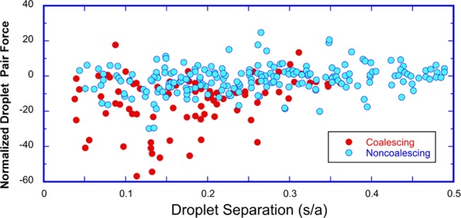
Plot of instantaneous normalized nondimensional electrostatic
force, F̃i,j calculated between droplet pairs in 2D emulsion configurations
as
obtained from captured images taken prior to any coalescence. The
nondimensional force F̃i,j is scaled by the Davis83 calculation of the force between a droplet pair aligned
with the field and at one radius separation, i.e.,  . Filled red (blue) circles indicate droplet
pairs that coalesce (do not coalesce) over an interval of 100 ms from
the time that the image configuration on which the forces are computed
is taken.
. Filled red (blue) circles indicate droplet
pairs that coalesce (do not coalesce) over an interval of 100 ms from
the time that the image configuration on which the forces are computed
is taken.
The interdroplet separation distances s/a plotted in Figure 6 are between 0.05 and 0.5. Separation distances s/a from 0.5 to about 2 are observed, but these typically correspond to pairs in which coalescence is not possible because of intervening neighbors (Figure 5b). For separations larger than approximately two with no intervening neighbors are present, but they are too far to coalesce in the 100 ms of observation from the frame capture. We also note that the shortest edge-to-edge separation distance observed in the plot is 0.05, which approaches the limit of the accuracy in the detection of the droplet edge (0.025).
Figure 6 makes clear
that large normalized, nondimensional attractive forces, from −20
to −40, develop between the droplets for separation s/a < 0.25. This is as expected, since
for the two-droplet problem, drops aligned with the field can, for
0.05 < s/a < 0.25, develop
attractive forces 10 to 100 times the force at one radius of separation
(the normalizing value in Figure 6). (See Figure 9 and the Atten et al.22 fit  for the two-droplet
forces.) For larger
values of the separation distance (0.5 > s/a > 0.25), the attractive forces drop off dramatically
to
the range of −10< F̃i,j < 0. This is also expected
due to the significant reduction in the dipolar force (Figure 9a). Repulsive forces (F̃i,j > 0) are small over the entire range of separation distances,
of
order 1–10. This is also in agreement with the repulsive interaction
force between two droplets aligned perpendicular to the field, where
the repulsive force in magnitude is 0.1.83 The calculated larger repulsive values are due to the attractive
interaction forces of neighboring droplets on the droplet pair, which
act to push the droplets away from each other.
for the two-droplet
forces.) For larger
values of the separation distance (0.5 > s/a > 0.25), the attractive forces drop off dramatically
to
the range of −10< F̃i,j < 0. This is also expected
due to the significant reduction in the dipolar force (Figure 9a). Repulsive forces (F̃i,j > 0) are small over the entire range of separation distances,
of
order 1–10. This is also in agreement with the repulsive interaction
force between two droplets aligned perpendicular to the field, where
the repulsive force in magnitude is 0.1.83 The calculated larger repulsive values are due to the attractive
interaction forces of neighboring droplets on the droplet pair, which
act to push the droplets away from each other.
Figure 9.

(a) Pair of isolated
droplets aligned with a uniform electric field
applied far away (up-to-down) and a color map of the electric field
in the uniform field direction as computed numerically (COMSOL). (b)
The nondimensionalized attractive force  exerted
on each of the pairs as a function
of the edge-to-edge separation s/a as computed from the COMSOL simulation and the bispherical analytical
solution83 and compared to the dipole approximation.
exerted
on each of the pairs as a function
of the edge-to-edge separation s/a as computed from the COMSOL simulation and the bispherical analytical
solution83 and compared to the dipole approximation.
From Figure 6, an assessment can be made on whether droplet pairs, which are calculated to be attractive in the instantaneous configuration in the images, do in fact coalesce in the 100 ms following the image capture. The figure indicates that almost all of the droplets with the largest attraction, |F̃i,j| > 20, which fall in the range s/a < 0.25, do coalesce. This is made clearer in a histogram plot, Figure 7a, of the count of the number of pairs, which coalesce (or do not coalesce), binned as a function of the normalized droplet pair force, |F̃i,j| > 20. The reason that the few pairs (3, cf. Figure 7a) that do not coalesce is the fact that one member of the pair coalesced with a member of another pair. However, less than half of the droplet pairs with smaller computed attractive forces, |F̃i,j| < 20, coalesces, even when the distance of separation is small (0.05 < s/a < 0.35). Pairs with even smaller attractions (|F̃i,j| < 10) and greater separations (0.35 < s/a < 0.5) do not coalesce at all.
Figure 7.
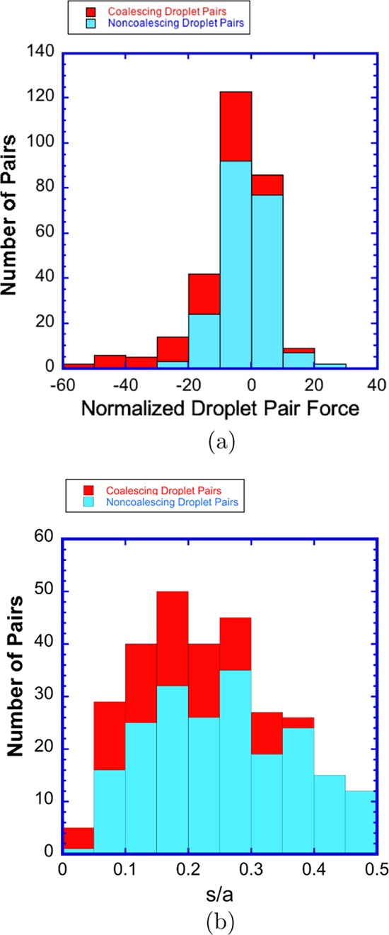
Histograms of the number of droplet pairs that coalesce or do not coalesce binned as a function of (a) normalized pairwise force F̃i,j and (b) separation distance s/a.
To understand these results, we
note that a coalescence event occurs
as droplet pairs approach to a critical distance where the field strength
is large enough that droplets deform significantly and join through
a liquid bridge, as seen in Figure 3. For the instantaneous configurations on which the
normalized attractive and repulsive forces are calculated, the measured
separation distances that are plotted are small (0.05 < so/a < 0.5). Coalescence
is achieved as long as the droplet pair, either initially or within
the 100 ms of observation, comes to a separation distance such that
the critical field strength (which is a function of the dipoles of
its neighbors) for coalescence is reached. To predict coalescence,
we can use the results on the merging of anchored droplets. As reviewed
in the introduction, in these studies (Atten et al.89), anchored, facing droplets are held at a fixed potential
difference V and positioned at initial separation
distances 10–3 < so/a < 1. The droplets deform and are found to
merge when the imposed potential difference V exceeds
a critical value Vcrit. The merging occurs
at a critical distance, scrit/a, which is approximately 0.6 so/a. At this critical distance, the Maxwell tensions
exerted by the normal electric field strengths at the facing poles
are large enough that equilibrium solutions for prolate shapes no
longer exist and droplets merge. This critical potential difference
is correlated in terms of a critical electrocapillary number, which
can be defined in terms of the electric field strength at the facing
poles of the droplet pair at the coalescence point, i.e.,  . This is equal to 0.2–0.4, depending
on the initial separation and the size of the capillary tips anchoring
the droplets to the droplet radii.
. This is equal to 0.2–0.4, depending
on the initial separation and the size of the capillary tips anchoring
the droplets to the droplet radii.
With the above as context,
consider first the droplet pairs with
a large net attractive force, |F̃i,j| > 20 (so/a < 0.25). By examining the droplet pairs
in this class, we observe that in most cases, the pair is aligned
along the field (or close to this orientation) and at a short enough
separation distance, so that the electric field at the facing poles
is large. In addition, in these cases, the neighbors are either located
at a far enough distance that they do not interact with the pair in
the calculation of the interdroplet force or are arranged around the
droplet pair perpendicular to the field so that only small repulsive
forces are exerted. In these cases, the field at the poles is large
enough that the critical capillary number is exceeded and the droplets
coalesce. From the color map in Figure 4b as an example and using the exact calculations, we
find that the droplets with large net attractive force (|F̃i,j| > 20) have electric
fields at their facing poles, which are 20–30 terms larger
than the applied field strength. The electrocapillary number corresponding
to the applied field strength of 250 V/mm and γ = 28 mN/m (the
value of the dynamic tension at the residence time for the droplets
in the wide chamber) is equal to  = 5 × 10⁻⁴ (using
the RMS value for the field). The droplets with large attractive force
|F̃i,j| > 20 (separations s/a <
0.25 and electric field amplification of 20–30 the applied
strength) have electrocapillary numbers in the range of 0.2–0.45.
This is in the interval for coalescence and explains why they coalesce.
It is also important to note that the electrocapillary numbers, at
the point of coalescence with amplification of the fields, are still
relatively small. Therefore, the droplets remain spherical until the
point of coalescence, as is evident in the images of Figure 3a,b, and this is true in all
of the remaining cases discussed below. The classes of droplets in Figure 6 with very small
mutual attraction forces |F̃i,j| < 10 and large separations 0.35 < s/a < 0.5, on examination, have electric
field values at their poles less than 10 times the applied strength.
This leads to electrocapillary numbers no greater than 0.05, insufficient
for coalescence.
= 5 × 10⁻⁴ (using
the RMS value for the field). The droplets with large attractive force
|F̃i,j| > 20 (separations s/a <
0.25 and electric field amplification of 20–30 the applied
strength) have electrocapillary numbers in the range of 0.2–0.45.
This is in the interval for coalescence and explains why they coalesce.
It is also important to note that the electrocapillary numbers, at
the point of coalescence with amplification of the fields, are still
relatively small. Therefore, the droplets remain spherical until the
point of coalescence, as is evident in the images of Figure 3a,b, and this is true in all
of the remaining cases discussed below. The classes of droplets in Figure 6 with very small
mutual attraction forces |F̃i,j| < 10 and large separations 0.35 < s/a < 0.5, on examination, have electric
field values at their poles less than 10 times the applied strength.
This leads to electrocapillary numbers no greater than 0.05, insufficient
for coalescence.
In the class of droplets in Figure 6 with small attractive forces
|F̃i,j| <20 for s/a < 0.35,
some merge and some do not.
An examination of the pairs in this category shows that the ones that
do not merge have field amplification at the poles, which are smaller
than 10, and hence electrocapillary numbers below the range required
for coalescence. The ones that do merge have the requisite amplification,
though, interestingly their attractive force is not as large as the
droplets in the class where |F̃i,j| > 20. Case by case examination
shows the coalescing pairs have neighbors in the field direction,
which are close enough to exert attractive forces that reduce the
net attractive interdroplet force between the pair. Thus, droplets
can merge even if the attraction is not large. For this same reason,
the few droplets pairs with net repulsion, which do merge in Figure 6 on examination,
have bounding neighbors in the field direction that exert strong attractions
on the pair members. This provides a resulting net repulsion between
the members, even though the field on the facing surfaces of the droplets
of the pair is large enough for coalescence. The above analysis of
the criteria for electrocoalescence does not take into account the
effect of the asphaltene film on the droplet interface on the coalescence.
When an asphaltene film is present with a large surface elasticity,
the elastic forces contribute to the restoring effects. This phenomenon
acts against the Maxwell stress, and thus the restoring forces due
to the tension are not the only surface restoring forces. The dynamics
of the interface for this case has not been studied in detail, but
a starting point would be to assume an equation of state for the tension,
which would include the elastic effect due to the stretching of the
asphaltene film. Following Rane et al.,17 we could start with their supposition that the Langmuir equation
of state is valid,  where Γ is the surface concentration
of the asphaltene, Γ∞ is the maximum packing
concentration of the asphaltene, and γo is the tension
in the absence of asphaltenes. As the area of the interface changes
during electrocoalescence, the surface concentration changes. If we
assume no additional adsorption during the time scale of the electrocoalescence
process, then the surface concentration is given by the conservation
equation, and the area expansion represents the strain on the film.
For this case, the elasticity of the layer, which would account for
the surface film, is
where Γ is the surface concentration
of the asphaltene, Γ∞ is the maximum packing
concentration of the asphaltene, and γo is the tension
in the absence of asphaltenes. As the area of the interface changes
during electrocoalescence, the surface concentration changes. If we
assume no additional adsorption during the time scale of the electrocoalescence
process, then the surface concentration is given by the conservation
equation, and the area expansion represents the strain on the film.
For this case, the elasticity of the layer, which would account for
the surface film, is  where Γo is the asphaltene
concentration at the point in which the field is applied. Following
in this way, two nondimensional groups would appear. The first group
is the electrocapillary number and a second group (
where Γo is the asphaltene
concentration at the point in which the field is applied. Following
in this way, two nondimensional groups would appear. The first group
is the electrocapillary number and a second group ( ) corresponding
to the ratio of the Maxwell
stress to the film elasticity. Note that in this formulation, the
surface concentration Γo is directly related to the
aging. For electrocoalesence, these ratios should exceed critical
values. We note that other elastomechanical expressions could be formulated
instead of the Langmuir equation of state, but in all cases, a second
group would appear representing a value for the characteristic Maxwell
stress to the characteristic film elasticity. Rane et al.17 undertake measurements of the film elasticity
by oscillating a pendant drop and find that Eo increases with the age of the drop, with values between 0
and 30 mN/m for aging between 0 and 120 min. Hence, the elasticity
is of the order of the tension. In our analysis, we base our criteria
for electrocoalescence on the values of Ec, stating that when Ec is large enough,
electrocoalescence occurs as the Mawell stresses are sufficiently
larger than the tension. Since the elasticity is the same order as
the tension, if Maxwell stresses are sufficiently large to exceed
the restoring force of tension, the same should be true for the restoring
force of elasticity. If the interfacial tension is extremely low (<1mN/m),
then the dominant effect would be the elastic resistance. Alternatively,
if the droplets are only aged a short amount of time, the elasticity
is very low and the dominant effect is the tension.
) corresponding
to the ratio of the Maxwell
stress to the film elasticity. Note that in this formulation, the
surface concentration Γo is directly related to the
aging. For electrocoalesence, these ratios should exceed critical
values. We note that other elastomechanical expressions could be formulated
instead of the Langmuir equation of state, but in all cases, a second
group would appear representing a value for the characteristic Maxwell
stress to the characteristic film elasticity. Rane et al.17 undertake measurements of the film elasticity
by oscillating a pendant drop and find that Eo increases with the age of the drop, with values between 0
and 30 mN/m for aging between 0 and 120 min. Hence, the elasticity
is of the order of the tension. In our analysis, we base our criteria
for electrocoalescence on the values of Ec, stating that when Ec is large enough,
electrocoalescence occurs as the Mawell stresses are sufficiently
larger than the tension. Since the elasticity is the same order as
the tension, if Maxwell stresses are sufficiently large to exceed
the restoring force of tension, the same should be true for the restoring
force of elasticity. If the interfacial tension is extremely low (<1mN/m),
then the dominant effect would be the elastic resistance. Alternatively,
if the droplets are only aged a short amount of time, the elasticity
is very low and the dominant effect is the tension.
3. Conclusions
This study has examined the process of electrocoalescence in a 2D emulsion of conducting water droplets in an insulating oil phase, which is generated in a microfluidic cell. An electric field applied across the emulsion induces charge separation and dipole formation in the conducting water droplets. The polarized droplets attract each other through dipolar forces, which intensify as the droplets approach to within a few tenths of a radius of each other. Petroleum crude is used for the oil because of the important applications of electrocoalescence to the removal of water from the crude. However, current interest is focused on the “droplet-based” microfluidic lab on chip applications that use electrocoalescence to combine droplets and break emulsions. Our microfluidic design uses flow focusing of water in oil to generate water droplets of uniform size, which are guided downstream as a single layer into a wide observation chamber. The 2D emulsion forms as the droplets collect in the chamber and an electric field is applied across the chamber to induce electrocoalescence. Our study provides two unique contributions: We demonstrate that our microfluidic design enables the electrocoalescence process in an opaque continuous phase to be visualized on the scale of the droplets with optical microscopy because the narrow chamber height allows the emulsion to become transparent. Electrocoalescence events are observed on an individual droplet basis, allowing an in situ examination of the merging process. Our study also demonstrates that the droplet scale data can be modeled to identify critical conditions for electrocoalescence using a local electrocapillary number. Numerical simulations for the electric field around the droplets in 2D configurations rendered directly from frame captures of microscopy images are obtained and used to compute the forces on the droplets. From the calculated forces, the mutual forces of attraction (or repulsion) between droplet pairs in the rendered images are examined as a function of the pair separation distance. These calculations are correlated with whether the droplet pair coalesced in the short (100 ms) time interval that followed from the captured frame on which the force calculation was based. Large mutual attractive forces at small separations (a few tenths of a droplet radius) correlated to electrocoalescence of the pair as the electric field between the droplets exceeded the value necessary for coalescence. Larger separations (approximately one-half of a radius) and very small attractive (or repulsive) forces correlated to noncoalescing droplets as the electric field strengths are too low. Almost all droplet pairs with repulsive interactions did not coalesce. For droplet pairs at close separation (a few tenths of a droplet radius) and intermediate values for mutual attraction, some pairs coalesced and some did not. An examination of the electric field on the droplet surfaces showed that for droplet pairs in this class that did coalesce the field strength between the droplets became large enough for coalescence. However, the net forces on each of the droplets (and hence the mutual force of attraction) were reduced because of the attractive interactions with neighboring droplets. Our demonstration that the electric field in a 2D emulsion can be computed exactly from rendered images and used to correlate coalescence events allows for a more in-depth study of the factors affecting electrocoalesence. This can open the possibility of programming the electrocoalesence process by manipulation of the applied electric field. Our approach of simulating directly the multiple droplet electrocoalescence to identify critical field strengths is also applicable to a three-dimensional study, although the visualization of the droplets in 3D would require other techniques such as pulsed field gradient (PFG) NMR since the 3D crude would be opaque in a microfluidic arrangement in which the channel height was larger to accommodate a 3D dispersion of droplets. The use of PFG-NMR to study water in crude oil emulsions has been undertaken by Sjoblom et al.99−101
4. Experimental Section
A petroleum crude (ExxonMobil) with εm = 2.5 and σm = 1.1 × 10⁻⁸ S/m (measured by an impedance analyzer, Agilent), viscosity μm = 0.023 kg m–1 s–1 (cone and plate viscometer), and density ρm = 8.75 × 10² kg/m3 is used, and the aqueous droplet phase is DI water with an assumed εp of 80, a measured σp of 1.2 × 10⁻⁵ S/m (conductivity meter), and ρp = 1.0 × 10³ kg/m3. The crude oil/DI water dynamic interfacial tension, γ, is measured using a pendant drop tensiometer (Kruss) and is shown in Figure 8. (All data at 20 °C, the temperature of experiments). The asphaltene content of the crude was obtained by extraction of the asphaltene with heptane (see e.g., ref (9) ASTM 863-69 standard), and the asphaltene content was 0.5 percent by weight and visually the crude appeared opaque.
Figure 8.
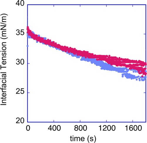
Dynamic interfacial tension between a crude oil droplet and DI water over a period of 2000 s; the graph shows three realizations.
The microfluidic cell is made using soft lithography102 and fabrication of two layers of polymerized
and cured PDMS. One layer containing the open fluidic channels and
chamber inscribed on one face is molded by curing PDMS (Sylgard 184,
Dow Corning) over a negative epoxy master of the fluidic features.
The second is a flat layer to seal the channel. The two layers are
bonded together following exposure to an oxygen plasma and mounted
on a standard glass microscope slide. Access ports cored into the
top layer using a biopsy punch allow the introduction of the oil and
aqueous streams via polyethylene tubing (1.5 mm OD) inserted into
the ports and connected to syringe pumps (Harvard Apparatus PHD).
The exit port allows the emulsion to exit through inserted tubing.
A monodisperse train of water droplets suspended in the crude is generated
by flow-focusing streams of crude and water through separate channels
from entry ports to an orifice where the droplets are formed. The
train is directed through a feeding channel to a holding chamber (width  = 3 mm and
length
= 3 mm and
length  = 10 mm) in
which the droplets arrange
themselves in an arbitrary configuration to form the 2D emulsion,
and in which the electric field is applied. Droplets leave the chamber
through an exiting channel ending in an exit port. Feeding and exit
channel widths to the chamber are 300 μm and 2 mm long, and
the height of the channels and chamber is
= 10 mm) in
which the droplets arrange
themselves in an arbitrary configuration to form the 2D emulsion,
and in which the electric field is applied. Droplets leave the chamber
through an exiting channel ending in an exit port. Feeding and exit
channel widths to the chamber are 300 μm and 2 mm long, and
the height of the channels and chamber is  = 60
μm, which (see below) is small
enough for the crude to be transparent. The flow-focusing orifice
is 50 μm in width, and at the flow rates of oil and water used
(qm = 0.2 μL/min and qp = 0.02 μL/min, respectively), droplets approximately
40 μm in diameter are generated. The droplets move through the
feeding channel and the chamber as a single layer. For the field generation,
planar electrodes of aluminum are inserted through the cell, perpendicular
to its lateral plane, and sited parallel to the chamber at a distance
= 60
μm, which (see below) is small
enough for the crude to be transparent. The flow-focusing orifice
is 50 μm in width, and at the flow rates of oil and water used
(qm = 0.2 μL/min and qp = 0.02 μL/min, respectively), droplets approximately
40 μm in diameter are generated. The droplets move through the
feeding channel and the chamber as a single layer. For the field generation,
planar electrodes of aluminum are inserted through the cell, perpendicular
to its lateral plane, and sited parallel to the chamber at a distance  . The electrodes
were connected to an amplifier
(TeK) controlled by a frequency generator (Agilent), which applied
a potential
. The electrodes
were connected to an amplifier
(TeK) controlled by a frequency generator (Agilent), which applied
a potential  across the electrodes.
To prevent accumulation
of charge and reduction of field strength, a sinusoidal AC rather
than a DC driving potential is applied across the electrodes. The
applied field is oscillated at a frequency ω = 500 Hz so that
across the electrodes.
To prevent accumulation
of charge and reduction of field strength, a sinusoidal AC rather
than a DC driving potential is applied across the electrodes. The
applied field is oscillated at a frequency ω = 500 Hz so that  and the free volume charge in the conducting
aqueous phase relaxes quickly relative to the inverse of the frequency.
Droplet coalescence events in the chamber are visualized by optical
microscopy using a microscope (Nikon) in the bright-field mode and
recorded with a high-speed camera (Redlake, 50 frames/s) with a 10×,
N.A. 1.4 (air) objective. The sensor has a pixel area of 1280 ×
1024, and the field of view in the observation cell was 1 mm ×
1 mm or a resolution of approximately 1 μm per pixel.
and the free volume charge in the conducting
aqueous phase relaxes quickly relative to the inverse of the frequency.
Droplet coalescence events in the chamber are visualized by optical
microscopy using a microscope (Nikon) in the bright-field mode and
recorded with a high-speed camera (Redlake, 50 frames/s) with a 10×,
N.A. 1.4 (air) objective. The sensor has a pixel area of 1280 ×
1024, and the field of view in the observation cell was 1 mm ×
1 mm or a resolution of approximately 1 μm per pixel.
The experiments are undertaken in a continuous flow-through mode.
The width of the chamber in the microfluidics device is much larger
than the width of the microchannel, which feeds the droplets into
the chamber. Therefore, the droplet movement in the chamber is relatively
slow, and the droplets appear to drift very slowly across the field
of view. At the oil flow rate qm used,
the characteristic velocity of the droplets in the channel is  ≈
200 μm/s and in the chamber
is ⟨v⟩ =
≈
200 μm/s and in the chamber
is ⟨v⟩ =  . In the absence of an
applied field, a
steady state is established, the field is then energized for a few
seconds, and a video of the coalescence dynamics in the chamber is
recorded from the moment the potential is applied. The field is then
turned off, and the slow flow in the chamber flushes the coalesced
drops out. The experiment is then repeated after microscopy observation
reveals there are no coalesced droplets in the chamber. Thus, for
the droplets observed in the chamber during an experiment, the approximate
time between their formation at the orifice and the initiation of
the field is approximately 500 s (
. In the absence of an
applied field, a
steady state is established, the field is then energized for a few
seconds, and a video of the coalescence dynamics in the chamber is
recorded from the moment the potential is applied. The field is then
turned off, and the slow flow in the chamber flushes the coalesced
drops out. The experiment is then repeated after microscopy observation
reveals there are no coalesced droplets in the chamber. Thus, for
the droplets observed in the chamber during an experiment, the approximate
time between their formation at the orifice and the initiation of
the field is approximately 500 s ( /⟨v⟩)
as the residence time
of the droplets in the channel feeding the chamber is only approximately
10 s (2 × 103 μm/200 μm/s). This 500 s time represents the approximate
“aging time” of the droplets from their formation at
the flow-focusing orifice. This time is important in applying the
results of this microfluidic electrocoalescence study to the operation
of field electrocoalescers. The residence time of the droplets in
the electrocoalescer from their point of formation is important as
it determines how long asphaltenes (and other surface-active material
in the oil) have been allowed to adsorb from the oil onto the droplet
surface. As we noted in the introduction, the greater this aging time
the more elastic the interfacial layer and the more difficult it becomes
for the droplets to merge. Conventional coalescers operate with a
residences time of 30–40 min103 to
deliver production rates of tens to hundreds of kilobarrales of oil/day.
Newer compact designs, which have improved the efficiency of the electrocoalescence
process, operate with lower holding volumes that have reduced this
residence time.6,7 The residence times of 10 min
in our experiments are of the order of the times for more compact
electrocoalescers, so our study reflects realistic conditions. More
importantly, the aging time can be increased (or adjusted to a desired
value) within our microfluidic chip design by using longer, serpentine-shaped
channels feeding into the chamber as undertaken by Nowbahar et al.24
/⟨v⟩)
as the residence time
of the droplets in the channel feeding the chamber is only approximately
10 s (2 × 103 μm/200 μm/s). This 500 s time represents the approximate
“aging time” of the droplets from their formation at
the flow-focusing orifice. This time is important in applying the
results of this microfluidic electrocoalescence study to the operation
of field electrocoalescers. The residence time of the droplets in
the electrocoalescer from their point of formation is important as
it determines how long asphaltenes (and other surface-active material
in the oil) have been allowed to adsorb from the oil onto the droplet
surface. As we noted in the introduction, the greater this aging time
the more elastic the interfacial layer and the more difficult it becomes
for the droplets to merge. Conventional coalescers operate with a
residences time of 30–40 min103 to
deliver production rates of tens to hundreds of kilobarrales of oil/day.
Newer compact designs, which have improved the efficiency of the electrocoalescence
process, operate with lower holding volumes that have reduced this
residence time.6,7 The residence times of 10 min
in our experiments are of the order of the times for more compact
electrocoalescers, so our study reflects realistic conditions. More
importantly, the aging time can be increased (or adjusted to a desired
value) within our microfluidic chip design by using longer, serpentine-shaped
channels feeding into the chamber as undertaken by Nowbahar et al.24
5. Computational Methods
To validate the COMSOL calculation of the electrostatic field in
the 2D emulsion of multiple water droplets in oil and the calculations
of the forces on the droplets, we first simulate the electric field
between two equally sized spherical droplets (radius a = 20 μm). The simulation is carried out for droplets in our
computational chamber with the center-to-center axis between the droplets
perpendicular to the top and bottom walls on which the potential difference  is applied. The bounding
surfaces of the
chamber are set to be far from the droplet pair (
is applied. The bounding
surfaces of the
chamber are set to be far from the droplet pair ( =
=  =
=  = 10a). This represents
the condition of a uniform electric field applied at infinity to two
isolated drops, as solved by Davis83 analytically
using bispherical coordinates. In Figure 9, we provide a color
map of the field strength in a slice perpendicular to the top and
bottom of the chamber. It contains the equatorial planes of both droplets
for the conductivity and viscosity ratios of our multidroplet water-in-oil
simulations (σ* = 10–3, ε* = 0.03).
Since the droplets are so much more conductive than the oil, their
electric fields are essentially zero in the droplets, as evident from
the map. The intensification of the field between the droplets, which
is the driving force of the electrocoalescence, is apparent with the
highest field strengths at the poles of the facing droplets. Quantitatively,
we obtain the attractive electrical force between the droplets, scaled
by
= 10a). This represents
the condition of a uniform electric field applied at infinity to two
isolated drops, as solved by Davis83 analytically
using bispherical coordinates. In Figure 9, we provide a color
map of the field strength in a slice perpendicular to the top and
bottom of the chamber. It contains the equatorial planes of both droplets
for the conductivity and viscosity ratios of our multidroplet water-in-oil
simulations (σ* = 10–3, ε* = 0.03).
Since the droplets are so much more conductive than the oil, their
electric fields are essentially zero in the droplets, as evident from
the map. The intensification of the field between the droplets, which
is the driving force of the electrocoalescence, is apparent with the
highest field strengths at the poles of the facing droplets. Quantitatively,
we obtain the attractive electrical force between the droplets, scaled
by  , (denoted by
  as in the introduction) through
the integration
of the normal electric field on the surface of the droplets. This
force is compared in Figure 9 with the exact analytical solution obtained by Davis.83 The agreement is excellent, demonstrating that
because of the very low conductivity ratio of the oil to the water
droplet phase, the field is essentially that of a continuous phase.
The agreement also provides confidence in our COMSOL solutions for
the multidroplet simulations. We also note that the dipole–dipole
approximation for the force is satisfactory for interdroplet separations s/a larger than one.
as in the introduction) through
the integration
of the normal electric field on the surface of the droplets. This
force is compared in Figure 9 with the exact analytical solution obtained by Davis.83 The agreement is excellent, demonstrating that
because of the very low conductivity ratio of the oil to the water
droplet phase, the field is essentially that of a continuous phase.
The agreement also provides confidence in our COMSOL solutions for
the multidroplet simulations. We also note that the dipole–dipole
approximation for the force is satisfactory for interdroplet separations s/a larger than one.
Acknowledgments
This work was partially supported by an NSF grant to the Center for the Exploitation of Nanostructures in Sensors and Energy Systems (CENSES), an Army Research Office grant ARO W911NF-11-1-0161, the Donors of the American Chemical Society Petroleum Research Fund, and ExxonMobil Research and Engineering Co.
Supporting Information Available
The Supporting Information is available free of charge at https://pubs.acs.org/doi/10.1021/acsomega.9b04259.
The authors declare no competing financial interest.
Supplementary Material
References
- Waterman L. Electrocoalescers. Chem. Eng. Prog. 1965, 61, 51–57. [Google Scholar]
- Galvin C. Design principles for electrocoalescers. IChemE Symp. Ser. 1986, 88, 101–113. [Google Scholar]
- Eow J.; Ghadiri M.; Sharif A.; Williams T. Electrostatic enhancement of coalecence of water droplets in oil: A review of the current understanding. Chem. Eng. J. 2001, 84, 173–192. 10.1016/S1385-8947(00)00386-7. [DOI] [Google Scholar]
- Eow J.; Gadhiri M. Electrostatic enhancement of coalescence of water droplets in oil: a review of the technology. Chem. Eng. J. 2002, 85, 357–368. 10.1016/S1385-8947(01)00250-9. [DOI] [Google Scholar]
- Lundgaard L.; Berg G.; Ingebrigtsen S.; Atten P.. Emulsions and Emulsion Stability; Sjoblom J., Ed.; Taylor and Francis, 2006; pp 549–592. [Google Scholar]
- Less S.; Vilagines R. The electrocoalescers’ technology: Advances, strengths and limitations for crude oil separation. J. Pet. Sci. Eng. 2012, 81, 57–63. 10.1016/j.petrol.2011.12.003. [DOI] [Google Scholar]
- Mhatre S.; Vivacquaa V.; Ghadiri M.; Abdullaha A.; Al-Marri M.; Hassanpour A.; Hewakandamby B.; Azzopardi B.; Kermani B. Electrostatic phase separation: a review. Chem. Eng. Res. Des. 2015, 96, 177–195. 10.1016/j.cherd.2015.02.012. [DOI] [Google Scholar]
- Mullins O. C. Review of the molecular structure and aggregation of asphaltenes and petroleomics. SPE J. 2008, 13, 48–57. 10.2118/95801-PA. [DOI] [Google Scholar]
- Mullins O. C. The asphaltenes. Ann. Rev. Anal. Chem. 2011, 4, 393–418. 10.1146/annurev-anchem-061010-113849. [DOI] [PubMed] [Google Scholar]
- Mullins O. C.; Sabbah H.; Eyssautier J.; Pomerantz A. E.; Barré L.; Andrews A. B.; Ruiz-Morales Y.; Mostowfi F.; McFarlane R.; Goual L. Advances in asphaltene science and the Yen-Mullins model. Energy Fuels 2012, 26, 3986–4003. 10.1021/ef300185p. [DOI] [Google Scholar]
- McLean J. D.; Spiecker P. M.; Sullivan A. P.; Kilpatrick P. K.. Structures and Dynamics of Asphaltenes; Springer, 1998; pp 377–422. [Google Scholar]
- Kilpatrick P. K. Water-in-crude oil emulsion stabilization: Review and unanswered questions. Energy Fuels 2012, 26, 4017–4026. 10.1021/ef3003262. [DOI] [Google Scholar]
- Ese M.-H.; Sjoblom J.; Fordedal H.; Urdahl O.; Ronningsen H. P. Ageing of interfacially active components and its effect on emulsion stability as studied by means of high voltage dielectric spectroscopy measurements. Colloids Surf., A 1997, 123, 225–232. 10.1016/S0927-7757(97)03963-0. [DOI] [Google Scholar]
- Yarranton H. W.; Hussein H.; Masliyah J. H. Water-in-hydrocarbon emulsions stabilized by asphaltenes at low concentrations. J. Colloid Interface Sci. 2000, 228, 52–63. 10.1006/jcis.2000.6938. [DOI] [PubMed] [Google Scholar]
- Verruto V. J.; Le R. K.; Kilpatrick P. K. Adsorption and molecular rearrangement of amphoteric species at oil- water interfaces. J. Phys. Chem. B 2009, 113, 13788–13799. 10.1021/jp902923j. [DOI] [PubMed] [Google Scholar]
- Pauchard V.; Rane J. P.; Zarkar S.; Couzis A.; Banerjee S. Long-term adsorption kinetics of asphaltenes at the oil-water interface: A random sequential adsorption perspective. Langmuir 2014, 30, 8381–8390. 10.1021/la500384r. [DOI] [PubMed] [Google Scholar]
- Rane J. P.; Zarkar S.; Pauchard V.; Mullins O. C.; Christie D.; Andrews A. B.; Pomerantz A. E.; Banerjee S. Applicability of the Langmuir equation of state for asphaltene adsorption at the oil-water interface: Coal-derived, petroleum, and synthetic asphaltenes. Energy Fuels 2015, 29, 3584–3590. 10.1021/acs.energyfuels.5b00179. [DOI] [Google Scholar]
- Qiao P.; Harbottle D.; Tchoukov P.; Masliyah J.; Sjoblom J.; Liu Q.; Xu Z. Fractionation of asphaltenes in understanding their role in petroleum emulsion stability and fouling. Energy Fuels 2017, 31, 3330–3337. 10.1021/acs.energyfuels.6b02401. [DOI] [Google Scholar]
- Eow J.; Ghadiri M. Drop-drop Coalescence in an electric field: The effects of applied electric field and electrode geometry. Colloids Surf., A 2003, 219, 253–279. 10.1016/S0927-7757(03)00051-7. [DOI] [Google Scholar]
- Chiesa M.; Melheim J.; Pedersen A.; Ingebrigtsen S.; Berg G. Forces acting on water droplets falling in oil under the influence of an electric field: numerical predictions versus experimental observations. Eur. J. Mech. B-Fluids 2006, 24, 717–732. 10.1016/j.euromechflu.2005.03.005. [DOI] [Google Scholar]
- Chiesa M.; Ingebrigtsen S.; Melheim J.; Hemmingsen P.; Hansen E.; Hestad O. Investigation of the role of viscosity on electrocoalescence of water droplets in oil. Sep. Purif. Technol. 2006, 50, 267–277. 10.1016/j.seppur.2005.12.003. [DOI] [Google Scholar]
- Atten P. Electrohydrodynamics of dispersed drops of conducting liquid: From drop deformation and interaction to emulsion evolution. Int. J. Plasma Environ. Sci. Technol. 2013, 7, 2–12. [Google Scholar]
- Yeganeh M.; Hegner J.; Lewandowski E.; Mohan A.; Lake L. W.; Cherney D.; Jusufi A.; Jaishankar A. In Capillary Desaturation Curve Fundamentals, SPE improved oil recovery conference. Tulsa, Oklahoma, USA, 2016.
- Nowbahar A.; Whitaker K. A.; Schmitt A. K.; Kuo T.-C. Mechanistic study of water droplet coalescence and flocculation in diluted bitumen emulsions with additives using microfluidics. Energy Fuels 2017, 31, 10555–10565. 10.1021/acs.energyfuels.7b01619. [DOI] [Google Scholar]
- Lin Y.-J.; Perrard A.; Biswal S. L.; Hill R. M.; Trabelsi S. Microfluidic investigation of asphaltenes-stabilized water-in-oil emulsions. Energy Fuels 2018, 32, 4903–4910. 10.1021/acs.energyfuels.8b00249. [DOI] [Google Scholar]
- Baroud C. N.; Gallaire F.; Dangla R. Dynamics of microfluidic droplets. Lab Chip 2010, 10, 2032–2045. 10.1039/c001191f. [DOI] [PubMed] [Google Scholar]
- Gu H.; Duits M.; Mugele F. Droplets formation and merging in two-phase flow microfluidics. Int. J. Mol. Sci. 2011, 122, 2572–2597. 10.3390/ijms12042572. [DOI] [PMC free article] [PubMed] [Google Scholar]
- Bremond N.; Bibette J. Exploring emulsion science with microfluidics. Soft Matter 2012, 8, 10549. 10.1039/c2sm25923k. [DOI] [Google Scholar]
- Huerre A.; Miralles V.; Jullien M. Bubbles and foams in microfluidics. Soft Matter 2014, 10, 6888–6902. 10.1039/C4SM00595C. [DOI] [PubMed] [Google Scholar]
- Theberge A. B.; Courtois F.; Schaerli Y.; Fischlechner M.; Abell C.; Hollfelder F.; Huck W. T. S. Microdroplets in microfluidics: An evolving platform for discoveries in chemistry and biology. Angew. Chem., Int. Ed. 2005, 49, 5846–5868. 10.1002/anie.200906653. [DOI] [PubMed] [Google Scholar]
- Urbanski J. P.; Thies W.; Rhodes C.; Amarasinghe S.; Thorsen T. Digital microfluidics using soft lithography. Lab Chip 2006, 6, 96–104. 10.1039/B510127A. [DOI] [PubMed] [Google Scholar]
- Huebner A.; Sharma S.; Srisa-Art M.; Hollfelder F.; Edel J. B.; deMello A. J. Microdroplets: A sea of applications. Lab Chip 2008, 8, 1244–1254. 10.1039/b806405a. [DOI] [PubMed] [Google Scholar]
- Teh S.-Y.; Lin R.; Hung L.-H.; Lee A. P. Droplet microfluidics. Lab Chip 2008, 8, 198–220. 10.1039/b715524g. [DOI] [PubMed] [Google Scholar]
- Chiu D.; Lorenz R.; Jeffries G. Droplets for ultra small-volume analysis. Anal. Chem. 2009, 81, 5111–5118. 10.1021/ac900306q. [DOI] [PMC free article] [PubMed] [Google Scholar]
- i Solvas X. C.; deMello A. Droplet microfluidics: recent developments and future applications. Chem. Commun. 2010, 47, 1936–1942. 10.1039/C0CC02474K. [DOI] [PubMed] [Google Scholar]
- Joensson H. N.; Andersson-Svahn H. Droplet microfluidics-a tool for protein engineering and analysis. Lab Chip 2011, 11, 4144–4147. 10.1039/c1lc90102h. [DOI] [PubMed] [Google Scholar]
- Joensson H. N.; Andersson Svahn H. Droplet microfluidics a tool for single-cell analysis. Angew. Chem., Int. Ed. 2012, 51, 12176–12192. 10.1002/anie.201200460. [DOI] [PubMed] [Google Scholar]
- Guo M. T.; Rotem A.; Heyman J. A.; Weitz D. A. Droplet microfluidics for high-throughput biological assays. Lab Chip 2012, 12, 2146–2155. 10.1039/c2lc21147e. [DOI] [PubMed] [Google Scholar]
- Seemann R.; Brinkmann M.; Pfohl T.; Herminghaus S. Droplet based microfluidics. Rep. Prog. Phys. 2012, 75, 016601 10.1088/0034-4885/75/1/016601. [DOI] [PubMed] [Google Scholar]
- Sesen M.; Alan T.; Neild A. Droplet control technologies for microfluidic high throughput screening (micro HTS). Lab Chip 2017, 17, 2372–2394. 10.1039/C7LC00005G. [DOI] [PubMed] [Google Scholar]
- Schwartz J. A.; Vykoukal J. V.; Gascoyne P. R. C. Droplet-based chemistry on a programmable micro-chip. Lab Chip 2004, 4, 11–17. 10.1039/b310285h. [DOI] [PMC free article] [PubMed] [Google Scholar]
- Kralj J.; Schmidt M.; Jensen K. Surfactant enhanced liquid-liquid Extraction in microfluidic channels with inline electric field enhanced coalescence. Lab Chip 2005, 5, 531–535. 10.1039/b418815b. [DOI] [PubMed] [Google Scholar]
- Ahn K.; Agresti J.; Chong H.; Marquez M.; Weitz D. A. Electrocoalescence of drops synchronized by size-dependent flow in microfluidic channels. Appl. Phys. Lett. 2006, 88, 264105–3. 10.1063/1.2218058. [DOI] [Google Scholar]
- Wang W.; Yang C.; Li C. Efficient on-demand compound droplet formation: From microfluidics to microdroplets as miniaturized laboratories. Small 2009, 5, 1149–1152. 10.1002/smll.200801598. [DOI] [PubMed] [Google Scholar]
- Niu X.; Gielen F.; deMello A. J.; Edel J. B. Electro-coalescence of digitally controlled droplets. Anal. Chem. 2009, 81, 7321–7325. 10.1021/ac901188n. [DOI] [PubMed] [Google Scholar]
- Zagnoni M.; Cooper J. M. On-chip electrocoalescence of microdroplets as a function of voltage, frequency and droplet size. Lab Chip 2009, 9, 2652–2658. 10.1039/b906298j. [DOI] [PubMed] [Google Scholar]
- Zagnoni M.; Lain G. L.; Cooper J. Electrocoalescence mechanisms of microdroplets using localized electric fields in microfluidic channels. Langmuir 2010, 26, 1443–14449. 10.1021/la101517t. [DOI] [PubMed] [Google Scholar]
- Gu H.; Murade C.; Duits M.; Mugele F. A microfluidic platform for on-demand formation and merging of microdroplets Using Electric Control. Biomicrofluidics 2011, 5, 011101 10.1063/1.3570666. [DOI] [PMC free article] [PubMed] [Google Scholar]
- Chokkalingam V.; Ma Y.; Thiele J.; Schalk W.; Tei J.; Huck W. An Electro-coalescence chip for effective emulsion breaking in droplet microfluidics. Lab Chip 2014, 14, 2398–2402. 10.1039/C4LC00365A. [DOI] [PubMed] [Google Scholar]
- Bhattacharjee B.; Vanapalli S. Electrocoalescence based serial dilution of microfluidic droplets. Biomicrofluidics 2014, 8, 044111 10.1063/1.4891775. [DOI] [PMC free article] [PubMed] [Google Scholar]
- Latham J.; Roxburgh I. Disintegration of pairs of water drops in an electric field. Proc. R. Soc. London, Ser. A 1966, 295, 84–97. 10.1098/rspa.1966.0227. [DOI] [Google Scholar]
- Taylor G. The coalescence of closely spaced drops when they are at different electric potentials. Proc. R. Soc. London, Ser. A 1968, 306, 423. 10.1098/rspa.1968.0159. [DOI] [Google Scholar]
- Brazier-Smith P.; Latham J. Numerical computations of the dynamics of disintegration of a drop Situated in an Electric Field. Proc. R. Soc. London, Ser. A 1969, 312, 277–289. 10.1098/rspa.1969.0153. [DOI] [Google Scholar]
- Brazier-Smith P.; Jennings S.; Latham J. An investigation of the behavior of drops and drop-pairs subjected to strong electrical forces. Proc. R. Soc. London, Ser. A 1971, 325, 363–366. 10.1098/rspa.1971.0174. [DOI] [Google Scholar]
- Atten P. Electrocoalescence of water drops in an insulating liquid. J. Electrost. 1993, 30, 259–270. 10.1016/0304-3886(93)90080-Q. [DOI] [Google Scholar]
- Zhang X.; Basaran O.; Wham R. Theoretical prediction of electric field enhanced coalescence of spherical drops. AIChE J. 1995, 41, 1629–1639. 10.1002/aic.690410704. [DOI] [Google Scholar]
- Baygents J.; Rivette N.; Stone H. Electrohydrodynamic Deformation and interaction of drop pairs. J. Fluid Mech. 1998, 368, 359–375. 10.1017/S0022112098001797. [DOI] [Google Scholar]
- Adamiak K. Interaction of two dielectric or conducting droplets aligned in the uniform electric field. J. Electrost. 2001, 51, 578–584. 10.1016/S0304-3886(01)00059-6. [DOI] [Google Scholar]
- Atten P.; Lundgaard L.; Berg G. A simplified model of electrocoalescence of two close water droplets in oil. J. Electrost. 2006, 64, 550–554. 10.1016/j.elstat.2005.10.009. [DOI] [Google Scholar]
- Mohammadi M.; Shahhosseini S.; Bayat M. Numerical study of the collision and coalescence of water droplets in an electric field. Chem. Eng. Technol. 2014, 37, 27–35. 10.1002/ceat.201200479. [DOI] [Google Scholar]
- Mohammadi M. Numerical and experimental study on electric field driven coalescence of binary falling droplets in oil. Sep. Purif. Technol. 2017, 176, 262–276. 10.1016/j.seppur.2016.12.015. [DOI] [Google Scholar]
- Mhatre S.; Deshmukh S.; Thaokar R. M. Electrocoalescence of a drop pair. Phys. Fluids 2015, 27, 092106 10.1063/1.4931592. [DOI] [Google Scholar]
- Bartlett C. T.; Généro G. A.; Bird J. C. Coalescence and break-up of nearly inviscid conical droplets. J. Fluid Mech. 2015, 763, 369–385. 10.1017/jfm.2014.664. [DOI] [Google Scholar]
- Lu J.; Fang S.; Corvalan C. M. Coalescence dynamics of viscous conical drops. Phys. Rev. E 2016, 93, 023111 10.1103/PhysRevE.93.023111. [DOI] [PubMed] [Google Scholar]
- Garzon M.; Gray L.; Sethian J. Electrohydrodynamic coalescence of droplets using an embedded potential flow model. Phys. Rev. E 2018, 97, 033112 10.1103/PhysRevE.97.033112. [DOI] [PubMed] [Google Scholar]
- Anand V.; Roy S.; Naik V. M.; Juvekar V. A.; Thaokar R. M. Electrocoalescence of a pair of conducting drops in an insulating oil. J. Fluid Mech. 2019, 859, 839–850. 10.1017/jfm.2018.849. [DOI] [Google Scholar]
- Anand V.; Patel R.; Naik V. M.; Juvekar V. A.; Thaokar R. M. Modelling and particle based simulation of electro-coalescence of a water-in-oil emulsion. Comput. Chem. Eng. 2019, 121, 608–617. 10.1016/j.compchemeng.2018.12.003. [DOI] [Google Scholar]
- Zhou Y.; Dong H.; Liu Y.-H.; Yang Z.-J.; Liu T.; Li M. Molecular dynamics simulations of the electrocoalescence behaviors of two unequally sized conducting droplets. Langmuir 2019, 35, 6578–6584. 10.1021/acs.langmuir.9b00744. [DOI] [PubMed] [Google Scholar]
- Allan R.; Mason S. Particle motions in sheared suspensions. XIV. Coalescence of liquid drops in electric and shear fields. J. Colloid Sci. 1962, 17, 383–408. 10.1016/0095-8522(62)90016-8. [DOI] [Google Scholar]
- Chabert M.; Dorfman K.; Viovy J. Droplet Fusion by Alternating Current (AC) Field Electrocoalescence in microchannels. Electrophoresis 2005, 26, 3706–3715. 10.1002/elps.200500109. [DOI] [PubMed] [Google Scholar]
- Thiam A. R.; Bremond N.; Bibette J. Breaking of an emulsion under an ac electric field. Phys. Rev. Lett. 2009, 102, 188304 10.1103/PhysRevLett.102.188304. [DOI] [PubMed] [Google Scholar]
- Priest C.; Herminghaus S.; Seemann R. Controlled electrocoalescence in microfluidics: Targeting a single lamella. Appl. Phys. Lett. 2006, 89, 134101–3. 10.1063/1.2357039. [DOI] [Google Scholar]
- Luo X.; Yin H.; Yan H.; Huang X.; Yang D.; He L. The electrocoalescence behavior of surfactant-laden droplet pairs in oil under a DC electric field. Chem. Eng. Sci. 2018, 191, 350–357. 10.1016/j.ces.2018.07.002. [DOI] [Google Scholar]
- Luo X.; Yin H.; Ren J.; Yan H.; Lü Y.; He L. Electrocoalescence criterion of conducting droplets suspended in a viscous fluid. J. Phys. Chem. C 2019, 123, 19588–19595. 10.1021/acs.jpcc.9b04357. [DOI] [Google Scholar]
- Bird J.; Ristenpart W.; Belmonte A.; Stone H. Critical Angle for Electrically driven coalescence of two conical droplets. Phys. Rev. Lett. 2009, 103, 164502 10.1103/PhysRevLett.103.164502. [DOI] [PubMed] [Google Scholar]
- Mohammadi M.; Shahhosseini S.; Bayat M. Electrocoalescence of binary water droplets falling in oil: Experimental study. Chem. Eng. Res. Des. 2014, 92, 2694–2704. 10.1016/j.cherd.2014.01.019. [DOI] [Google Scholar]
- Xia Y.; Reboud J.-L. Hydrodynamic and electrostatic interactions of water droplet pairs in oil and electrocoalescence. Chem. Eng. Res. Des. 2019, 144, 472–482. 10.1016/j.cherd.2019.02.012. [DOI] [Google Scholar]
- Jones T. B.; Jones T. B.. Electromechanics of Particles; Cambridge University Press, 2005. [Google Scholar]
- Pethig R. Review Article—Dielectrophoresis: Status of the the theory, technology and applications. Biomicrofluidics 2010, 4, 022811 10.1063/1.3456626. [DOI] [PMC free article] [PubMed] [Google Scholar]
- Kirby B. J.Micro-and Nanoscale Fluid Mechanics: Transport in Microfluidic Devices; Cambridge University Press, 2010. [Google Scholar]
- Pethig R. R.Dielectrophoresis: Theory, Methodology and Biological Applications; John Wiley & Sons, 2017. [Google Scholar]
- Eow J.; Ghadiri M.; Sharif A. Experimental studies of deformation and break-up of aqueous drops in high electric fields. Colloids Surf., A 2003, 225, 193–210. 10.1016/S0927-7757(03)00330-3. [DOI] [Google Scholar]
- Davis M. H. Two charged spherical conductors in a unifrom electric field: forces and field strength. Q. J. Mech. Appl. Math. 1964, 17, 499–511. 10.1093/qjmam/17.4.499. [DOI] [Google Scholar]
- Taylor G. Disintegration of water drops in am electric field. Proc. R. Soc. London, Ser. A 1964, 280, 383–397. 10.1098/rspa.1964.0151. [DOI] [Google Scholar]
- Stone H.; Lister J.; Brenner M. Drops with conical ends in electric and magnetic fields. Proc. R. Soc. London, Ser. A 1999, 455, 329–347. 10.1098/rspa.1999.0316. [DOI] [Google Scholar]
- Rhodes A.; Yariv E. The elongated shape of a dielectric drop deformed by a strong electric field. J. Fluid Mech. 2010, 664, 286–296. 10.1017/S0022112010004581. [DOI] [Google Scholar]
- Ristenpart W.; Bird J.; Belmonte A.; Dollar F.; Stone H. Non-Coalescence of oppositely charged drops. Nat. Lett. 2009, 461, 377–380. 10.1038/nature08294. [DOI] [PubMed] [Google Scholar]
- Hamlin B.; Creasey J.; Ristenpart W. Electrically tunable partial coalescence of oppositely charged drops. Phys. Rev. Lett. 2012, 109, 094501 10.1103/PhysRevLett.109.094501. [DOI] [PubMed] [Google Scholar]
- Raisin J.; Reboud J.; Atten P. Electrically induced deformations of water-air and water-oil interfaces in relation to electrocoalescence. J. Electrost. 2011, 69, 275–283. 10.1016/j.elstat.2011.03.017. [DOI] [Google Scholar]
- Wang J.; Wang B.; Qiu H. Coalescence and breakup of oppositely charged droplets. Sci. Rep. 2014, 4, 7123 10.1038/srep07123. [DOI] [PMC free article] [PubMed] [Google Scholar]
- Liu Z.; Wyss H. M.; Fernandez-Nieves A.; Shum H. C. Dynamics of oppositely charged emulsion droplets. Phys. Fluids 2015, 27, 082003 10.1063/1.4928854. [DOI] [Google Scholar]
- Liu Z.; Chan S. T.; Faizi H. A.; Roberts R. C.; Shum H. C. Droplet-based electro-coalescence for probing threshold disjoining pressure. Lab Chip 2015, 15, 2018–2024. 10.1039/C5LC00177C. [DOI] [PubMed] [Google Scholar]
- Anand V.; Juvekar V. A.; Thaokar R. M. Modes of coalescence of aqueous anchored drops in insulating oils under an electric field. Colloids Surf., A 2019, 568, 294–300. 10.1016/j.colsurfa.2019.02.002. [DOI] [Google Scholar]
- Chen X.; Liu P.; Qi C.; Wang T.; Liu Z.; Kong T. Non-coalescence of oppositely charged droplets in viscous oils. Appl. Phys. Lett. 2019, 115, 023701 10.1063/1.5109181. [DOI] [Google Scholar]
- Szymborski T.; Korczyk P.; Holyst R.; Garstecki P. Ion Polarization of liquid-liquid interfaces; Dynamic control of the rate of electro-coalescence. Appl. Phys. Lett. 2011, 99, 094101 10.1063/1.3629783. [DOI] [Google Scholar]
- Baret J.-C. Surfactants in droplet-based microfluidics. Lab Chip 2011, 12, 422–433. 10.1039/C1LC20582J. [DOI] [PubMed] [Google Scholar]
- Gaiser P.; Binz J.; Gompf B.; Berrier A.; Dressel M. Tuning the dielectric properties of metallic-nanoparticle/elastomer composites by strain. Nanoscale 2015, 7, 4566–4571. 10.1039/C4NR06690A. [DOI] [PubMed] [Google Scholar]
- Saville D. A. Electrohydrodynamics: The Taylor-Melcher leaky dielectric model. Annu. Rev. Fluid Mech. 1997, 29, 27–64. 10.1146/annurev.fluid.29.1.27. [DOI] [Google Scholar]
- Balinov B.; Urdahl O.; Soderman O.; Sjoblom J. Characterization of water-in-crude oil emulsions by the NMR self-diffusion technique. Colloids Surf., A 1994, 82, 173–181. 10.1016/0927-7757(93)02618-O. [DOI] [Google Scholar]
- Hjartnes T. N.; Mhatre S.; Gao B.; Sørland G. H.; Simon S.; Sjöblom J. Demulsification of crude oil emulsions tracked by pulsed field gradient NMR. Part II: Influence of chemical demulsifiers in external AC electric field. Colloids Surf., A 2019, 586, 124188 10.1016/j.colsurfa.2019.124188. [DOI] [Google Scholar]
- Hjartnes T. N.; Sørland G. H.; Simon S.; Sjöblom J. Demulsification of Crude Oil Emulsions Tracked by Pulsed Field Gradient (PFG) Nuclear Magnetic Resonance (NMR). Part I: chemical demulsification. Ind. Eng. Chem. Res. 2019, 58, 2310–2323. 10.1021/acs.iecr.8b05165. [DOI] [Google Scholar]
- McDonald J. C.; Duffy D. C.; Anderson J. R.; Chiu D. T.; Wu H. K.; Schueller O. J. A.; Whitesides G. M. Fabrication of microfluidic systems in poly(dimethylsiloxane). Electrophoresis 2000, 21, 27–40. . [DOI] [PubMed] [Google Scholar]
- Urdahl O.; Wayth N. I.; Fórdedal H.; Williams T. J.; Bailey A. G.. Encyclopedic Handbook of Emulsion Technology; CRC Press, 2001; pp 678–693. [Google Scholar]
Associated Data
This section collects any data citations, data availability statements, or supplementary materials included in this article.