Obtaining Tertiary Protein Structures by the ab Initio Interpretation of Small Angle X-ray Scattering Data

Abstract

Small angle X-ray scattering (SAXS) is an important tool for investigating the structure of proteins in solution. We present a novel ab initio method representing polypeptide chains as discrete curves used to derive a meaningful three-dimensional model from only the primary sequence and SAXS data. High resolution structures were used to generate probability density functions for each common secondary structural element found in proteins, which are used to place realistic restraints on the model curve’s geometry. This is coupled with a novel explicit hydration shell model in order to derive physically meaningful three-dimensional models by optimizing against experimental SAXS data. The efficacy of this model is verified on an established benchmark protein set, and then it is used to predict the lysozyme structure using only its primary sequence and SAXS data. The method is used to generate a biologically plausible model of the coiled-coil component of the human synaptonemal complex central element protein.

Introduction

Biological small angle X-ray scattering (BioSAXS) is an increasingly important method for characterizing protein structures in solution.¹⁻³ Its primary advantage over techniques such as crystallography and NMR is its ability to provide information under native conditions about large protein molecules not accessible by complementary methods. However, there is a price to pay for this advantage: the random motion and orientation of molecules in solution leads to a loss of information due to an effective averaging of the scattering, leaving only information about the protein’s intramolecular distances, not their spatial orientations.⁴ Because of these challenges, correctly interpreting BioSAXS data to realize meaningful results remains a challenging task.⁵

Two main methods have been developed to interpret BioSAXS data. The first assumes an accurate three-dimensional (3D) model of the protein backbone, usually derived from X-ray crystallography.⁶⁻⁹ This model is used to calculate the X-ray scattering curve once the excluded solvent volume is taken into account. A major advance, first presented in the CRYSOL algorithm,⁶ was the inclusion of the solvation layer—the ordered water molecules at the surface of the protein. CRYSOL and the FoXS package, which was developed by Schneidman-Duhovny et al.,⁷ adjust an implicit “shell” of scattering (“implicit” meaning they do not model individual solvent molecules). Other packages treat the shell explicitly using either molecular dynamics (AquaSAXS)⁸ or a geometric filling approach (the SCT suite).⁹ Allowing for a shell that can have gaps and fill cavities in the protein model gives a more reliable fit to the data.⁵ An extension of this approach is to use all atomistic modeling with Protein Data Bank (PDB) structures as a starting point.^10,11 The application of such techniques, however, can require significant technical expertise. The second method does not assume an initial structure (ab initio) but simplifies the protein model as either a volume¹² or a chain¹³ of scattering beads without explicit secondary structure. These methods are hence applicable to de novo structural prediction, but the lack of secondary structure means interpreting these predictions is a difficult task.⁵

Here we propose an alternative ab initio technique that uses a curve model of the 3D structure of the polypeptide chain. This description has a much reduced number of parameters by comparison to all atomistic models. Similar curve models have been previously proposed¹⁴⁻¹⁶ but not applied to the interpretation of BioSAXS data. The model is parametrized by consecutive discretized descriptions of the four major secondary structural elements: α-helices, β-strands, flexible sections, and random coils. The permissible geometry of these curves is restricted by empirically determined constraints, which are akin to Ramachandran constraints.¹⁷ To use the model for the interpretation of BioSAXS data, the polypeptide chain model is combined with a water model for the first hydration shell and an empirically calibrated scattering model. The geometry of the model can then be optimized against the experimental BioSAXS data. A critical factor, novel to our curve representation of the polypeptide chain, is the construction of empirical probability distributions for the model parameters. These distributions serve the dual purpose of preferencing commonly observed secondary structures in the set of potential chain models, while simultaneously allowing for predictions with rare/novel but physically permissible secondary structure. An advantage of this method for ab initio interpretation of BioSAXS data, by comparison to the established bead models,^12,13 is that by accurately characterizing the protein’s secondary structure it can reliably incorporate additional structural information in order to improve the results of the technique. In this study, contact predictions, based on sequence alignments alone, are used to improve the model predictions. A final advantage of the code developed is that its only input requirements are the primary sequence and scattering data, so it places only basic technical requirements on the user for its use.

We first applied this new methodology to data of well-characterized model protein lysozyme before moving to the BioSAXS data of the structural core of the human synaptonemal complex central element protein 1 (SYCE1). This protein represents an essential structural component of the synaptonemal complex (SC) that binds together homologous chromosomes during meiosis and provides the necessary three-dimensional environment for crossover formation.¹⁸⁻²⁰ The SC is formed of oligomeric α-helical coiled-coil proteins that undergo self-assembly to create a latticelike assembly.²¹⁻²³ In a recent biochemical and biophysical study, human SYCE1 was shown to adopt a homodimeric structure in which its structural core is provided by residues 25–179 forming an antiparallel coiled coil.²⁴ Further, the structural core was expressed in an engineered construct in which two SYCE1 25–179 sequences were tethered together through a short linker sequence (GQTNPG). This construct faithfully reproduced the native structure, and substantially improved protein stability in solution²⁴ (by comparison to the unlinked core). In this study, using secondary structure predictions and distance restraints purely based on the sequence of the protein alone, an excellent model of an antiparallel extended but bent coiled coil is derived, which is fully consistent with biological data.

Methods

First we describe the reduced parameter protein model we use to interpret BioSAXS data. This is composed of a polypeptide chain curve model with a surrounding explicit hydration shell. Empirically calibrated structure factor functions for each constituent element of the model are constructed to produce theoretical scattering curves for this tertiary structure model.

Polypeptide Chain

The polypeptide chain is represented as a set of points in 3D space {c_i}_i=1ⁿ, the positions of the C^α atoms in each amino acid. The geometry of four consecutive points (c_i, c_i+1, c_i+2, c_i+3) can be characterized by two parameters: the curvature κ and torsion τ. κ is defined by the unique sphere made by the center of the joining edges (see Figure 1a); the smaller the sphere the more tightly the curves joining the points fold on themselves. τ is determined by how sharply the curve bends away from its plane of curvature, and its sign denotes the curve section’s chirality (it is positive for right-handed coiling and negative for left-handed coiling). More precise definitions are as follows.

Figure 1.

Figures depicting elements of the backbone model. (a) Curve subsections (c_i, c_i+1, c_i+2, c_i+3) (red points) and their midsection points (c_m1, c_m2, c_m3) (blue). The first example is more tightly wound and has a smaller sphere, hence a higher κ value. The sphere defined by these midsection points is shown; the inverse of its radius is the curvature κ. (b) α-Helical section with uniformly similar (κ, τ) values. (c) Flexible (linker) section with varying (κ, τ) values.

Curvature κ

A section of four residues defined by the points (c_i, c_i+1, c_i+2, c_i+3) defines three edges with midpoints c_ml = (c_i+l–1 + c_i+l)/2, which in turn define the curvature sphere.¹⁻³ The curvature, the inverse of its radius, is

1

where θ₁₂₃ is the angle between the vectors c_m1 – c_m3 and c_m2 – c_m3.

Torsion τ

Three points define a plane (with unit normal vector n), and the four points (c_i, c_i+1, c_i+2, c_i+3) define two planes through their unit normal vectors n₂ and n₂, respectively:

2

The torsion is the (length weighted) angle these planes make with each other:

3

with θ_n is the angle between n₁ and n₂; see, e.g., ref (25).

The algorithm for generating a curve of length n from n – 3 pairs of values of (κ_i, τ_i) is as follows: Consider a section of curve of length m and m – 3 pairs (κ_i, τ_i), whose three initial points c₁, c₂, and c₃ are randomly chosen (with fixed separation distance R = 3.8). Since scattering expressions are invariant under an arbitrary translation and rotation,⁴ the exact values of the first two points do not matter (as long as their separation is R). The third point is a structural degree of freedom, but it is restricted such that the C^α–C^α distance between c₁ and c₃ is greater than R. Once these points are specified the fourth point will be

4

with θ = ∈ [0, π], ϕ ∈ [0, 2π]. The set (c₁, c₂, c₃, θ, ϕ) defines four points and hence κ and τ values. Using values of κ₁ and τ₁, eqs 1 and 3 are solved for θ and ϕ; this gives c₄. The next point c₅ can similarly be found from the values κ₂ and τ₃, and so on until all m – 3 (κ_i, τ_i) have been used to yield the m points c_i. Examples of an α-helical and flexible linker sections (taken from the structure of bovine serum albumin (PDB 3V03)²⁶) are shown in Figure 1b,c.

Secondary Structure Geometry Restraints

In order to derive geometric constraints, C^α coordinates were extracted from a set of over 60 protein structures for which high resolution crystal structures are available in the PDB and the κ and τ values calculated for all subsections (c_i, c_i+1, c_i+2, c_i+3). The κ–τ pairs are shown in Figure 2a. There are three main populations of values (preferential regions). As shown in section 1.3 of the Supporting Information, these regions of (κ, τ) space correspond to the three preferential domains of Ramachandran space.¹⁷ Using the PDB’s secondary structure annotation, this data was split into categories of β-strands, α-helices, and the rest which are not identified (referred to here as linkers). To account for random coils, the data was further divided into subsets whose values remained in one preferential domain (as in Figure 1b) and those whose κ–τ values belong to multiple domains (as in Figure 1c). For each set of data a representative probability density function (PDF) was calculated using kernel smoothing techniques²⁷ (for details see sections 1.4 and 1.5 of the Supporting Information); an example is shown in Figure 2b.

Figure 2.

Illustrations of κ–τ spaces used to impose realistic geometry constraints on the polypeptide chain. (a) (κ, τ) pairs obtained from crystal structures, plotted as points with κ on the horizontal axis and τ on the vertical axis. (b) PDF, created from the data in (a), which correspond to linker sections. There are three distinct domains of high probability corresponding to the preferred secondary structural elements.

Generating Models from Secondary Structure Annotation

In order to generate models based on secondary structure information alone, a protein of n amino acids is split into l distinct subdomains of length m_i (∑_i=1^l m_i = n). Each section l is classified as α-helical, β-strand, or linker; for the purpose of testing and calibration the PDB file’s secondary structure assignment was used to perform this task. For each section of length m_i, m_i – 3 (κ, τ) pairs are drawn from an appropriate PDF and the section is constructed. This process creates the l individual sections of secondary structure elements, which must then be linked together. Two neighboring sections with specified geometry (for example, an α-helix and linker) still have a relative rotational degree of freedom. To ensure this remains physically realistic, the geometry of the last three and first C^α positions of neighboring secondary sections were extracted from the PDB set and further PDFs for the set of permissible (κ, τ) pairs of these joining sections were generated for each type of join (i.e., α-helix to linker or linker to β-strand). Therefore, the final step of the process is to obtain all (κ, τ) values for the joint geometry and then construct the whole backbone. A precise mathematical description of this algorithm, constrained backbone algorithm (CB), is given in section 1.6 of the Supporting Information. One example of a structure generated using this algorithm is shown in Figure 6b; this particular structure was used as a starting point for an ab initio structure optimization in this study.

Figure 6.

Secondary knot fingerprint analysis of the lysozyme structure. (a) C^α trace of lysozyme (PDB 1LYZ(41)). The α-helices are shown in red, β-strand structures are in green, and linker sections are in light blue. (b) Random structure generated using the CB algorithm which has the same secondary structural elements as lysozyme. This could be a starting model for the fitting procedure. Panels c and d are secondary fingerprints of two different crystal structures of lysozome (1LYZ and 1AKI, respectively). The knot types are indicated (Rolfsen classification⁴²); white spaces indicate no secondary knots (all knots were of the primary type). (e) Secondary fingerprint for the random structure shown in (b); it differs significantly from (c) and (d) and has a larger range of knots present.

The Hydration Layer

Once the curve representation is obtained, it is crucial to include a model of the hydration layer in order to generate realistic scattering curves. To this aim, solvent molecules are placed between a pair of cylindrical surfaces surrounding the axis of a section of the backbone (Figure 3a). This layer is then reduced by removing all overlapping solvent molecules. This ensures the shell remains in hollow sections between the fold and on the protein surface, while the water molecules are removed from significantly folded regions. This is a crucial aspect of our hydration layer model, as it has been shown that one needs to allow for inhomogeneous hydration layers in order to avoid inaccurate predictions from BioSAXS data.²⁸ This method is illustrated in Figure 3, where the two cylinders of radius R_c (core) and R_o (outer), R_o > R_c, are centered on a section i’s helical axis (Figure 3a). Consider a solvent molecule belonging to another section j whose nearest distance from the axis of section i is R_s. If R_s < R_c, the solvent is too close to the backbone and removed. If R_c < R_s < R_o, the solvent is classed as being shared by the sections i and j and only counted once.

Figure 3.

Visualizations of the hydration layer model. (a) Initial solvent layer, shown as silver spheres with the core R_c and outer R_o cylinders surrounding the axis of the section (red curve). (b) Overlapping sections and solvent layers. (c) In blue, the removed solvent molecules of the pair of sections shown in (b).

This process is applied to all solvent molecules from sections i and j on each other; an example of the outcome is shown in Figure 3b,c. Applying this process pairwise to all sections of a C^α backbone yields the final hydration layer. The exact mathematical description of this hydration layer is detailed in sections 2.1–2.3 of the Supporting Information. The values of the radii (R_c, R_o) and a number of other parameters controlling the solvent density were determined by fitting the model to high resolution crystal structures which contained the first hydration shell. An example model shell, generated with these parameters, is shown in comparison to the model solvent positions from the subatomic resolution structure of a phosphate binding protein from the PDB 4F1V(29) in Figure 4. It is shown the two distributions are statistically similar in section 2.4 of the Supporting Information and hence that the model is a realistic representation of the average positions of the inner hydration shell.

Figure 4.

Comparisons of crystallographic and model solvent positions from the crystal structure of a phosphate binding protein PDB 4F1V, determined at ultrahigh resolution of 0.88 Å.²⁹ (a) PDB backbone and relevant solvent molecules. (b) Model solvent positions (surrounding the same curve as in (a)) obtained with the experimentally determined hydration shell model parameters.

Scattering Formula

Once the polypeptide chain and hydration layer models are determined, the Debye formula³⁰

5

is used to calculate the scattered intensity I(q) as a function of momentum transfer, q = π sin(θ)/λ. Here N is total number of C^α atoms and solvent molecules and f_i(q) is the form factor for residue i. There are two types, one for an amino acid with an excluded volume correction and one for a solvent molecule, which are defined in the following section.

Amino Acid Form Factors

The form factor f_am of an amino acid, centered on the C^α atom position, is

6

where f_b is the scattering of the amino acid in a vacuum, f_ex is the adjustment due to the excluded volume of solvent, and ρ_ex is a constant. Each amino acid is assigned the same scattering function f_b(q), a five-factor exponential representation:

7

where {A_i, B_i}_i=1⁵ and C are empirically determined constants (a standard form used to fit molecular form factors³¹). The excluded volume effect is captured using an exponential model in the form

8

where r_w is the average atomic radius of the atom.^6,7,13 To calculate the excluded volume for amino acids, coordinates for all 20 amino acids³² and values of r_w for carbon, nitrogen, oxygen, hydrogen, and sulfur (e.g., ref (33)) were used to compute the excluded volume scattering, centered at the C^α, through

9

where r_i^α is the distance of atom i from the C^α molecule and N_am is the number of atoms in the amino acid. Since f_b does not discriminate individual amino acids, this value f_ex was averaged over all 20 amino acids, weighted by their abundance in globular proteins (see ref (34)). This averaged function, shown in Figure 5e, gives f_ex(q). Finally, eq 6 includes a constant ρ_ex which modulates the effect of the excluded volume scatter by comparison to f_b; this value is constrained to lie within 0.75 and 1.25 (similar constraints are used in refs (6, 7, and 13)). The scattering form for an individual water molecule in the hydration layer is

10

where f_hy and f_ox are the vacuum scatterings of hydrogen and oxygen, respectively.³¹ The constant ρ_h was empirically determined (as in ref (7)). A detailed description of the parameter determination method is given in section 3 of the Supporting Information.

Figure 5.

Fits to scattering data for various molecules using appropriate C^α coordinates as a backbone model {c}_i=1ⁿ. (See section 3 of the Supporting Information for details.) In panels a–d, the data scattering data is shown overlaid by the smoothed data used for fitting (blue curve) and the model fit (red curve). Panel e is the averaged scattering function f_am obtained by averaging the scattering parameters obtained from fits like those shown in (a)–(d).

Evaluating Structural Similarity

In the next step the geometry of each model generated by the CB algorithm is optimized by refinement against the scattering data. However, since the problem is under-determined, many models will fit the experimental data, so a method is required to compare structures and determine which predictions are “essentially the same” in that they only differ by small local conformational changes (as one should expect in solution). The standard methods in protein crystallography for comparing similar protein structures are based on root-mean-squared deviations (RMSDs) where two structures are superimposed to minimize the sum of all distances of equivalent paired atoms.^35,36 This measure and variants on it are known to be overly sensitive to large deviations in single loops (as discussed in ref (35)). Unlike homologous crystal structures, which will often only differ by the change in a small subsection of the whole structure, the comparison here will be made between structures generated by a random algorithm, so the significant buildup of relatively small individual RMSD errors is likely. In section 2.1 of the Supporting Information, a number of additional problems with using the RMSD measure in this context are discussed in detail. To mitigate these problems, a novel and more robust approach based on knot theoretical techniques was developed.

Knot Fingerprints

Techniques from knot theory have previously been applied to identify specific (knotted) entanglements in protein structures.³⁷ To compare two protein structures using knot theory, the N- and C- termini need to be joined.³⁸ As demonstrated in ref (37), a sensible procedure for making this extension is to surround the backbone with a sphere, then choose two random points on the sphere and join the end termini to these points; finally, this extended curve is closed with a geodesic arc. The knot is then classified (e.g., via Jones polynomials). This procedure is repeated a significant number of times (10 000 in this study), and the most common knot (MCK) is chosen to indicate the knotting of the curve. To obtain additional information, the MCK is calculated for all subsets {c_i|i = k, k + 1, ..., j, j > k, j – k > 3} of the curve. One can then plot this data on a “staircase” diagram with j and k on the axes and each square of the domain colored by its most common knot (e.g., ref (39)) (examples of staircase diagrams are shown in Figure 6c–e). The fingerprint is found to be preserved across protein families,³⁹ even when there is low sequence identity.⁴⁰

Secondary Knot Fingerprints

Figure 6c is the knot fingerprint for one set of lysozyme coordinates (shown in Figure 6a), of the second most common knot identified during the random closure process. The secondary fingerprint shown in Figure 6d is from a second set of lysozyme coordinates; panels c and d of Figure 6 are significantly similar. The secondary fingerprint (Figure 6e) is derived from a CB generated backbone model, shown in Figure 6b, which has the same secondary structure sequence as 1LYZ. The secondary fingerprint differences between the correct structure (Figure 6c) and the randomly generated structure (Figure 6d) is immediately obvious. All primary fingerprints in these cases are identical, and all have the unknot as the most common knot. It is clear secondary (and possibly tertiary) knot fingerprints can differentiate unknotted folds. A knot fingerprint statistic is defined in section 4.2 of the Supporting Information which quantifies the weighted similarity of knot fingerprints at level l associated with the curves K₁ and K₂ (l = 2 for Figures 6c–e); it yields a value between 0, completely dissimilar, and 1, identically folded.

In section 4.3 of the Supporting Information it is demonstrated that the statistic has the following properties. First, it quantifies crystal structures of the same molecule as highly similar, , and randomly generated structures (with the same secondary structure sequence) as significantly dissimilar, generally (see Figure 7a). Second, it judges crystal monomer structures of different proteins with different 3D structures but with similar lengths as being significantly different (typically ); i.e. it can differentiate folds. Third, it is shown to have excellent properties under deformation. To demonstrate, n randomly distributed changes were applied to a lysozyme crystal structure K_pdb using the CB algorithm. For each n, 50 such structures K_n were generated and the values of the statistic were calculated. The results are plotted as a function of n in Figure 7b. The mean value drops off rapidly to the same value as the average of the randomly generated structures (after about 15 changes). The maximum value always remains significantly higher than the mean; it drops below PDB quality after only two changes. Therefore, a high value of >0.75 indicates the structure is likely largely the same as the original structure.

Figure 7.

Properties of the (secondary) knot fingerprint statistic based on variations of the lysozyme structure. (a) Secondary knot statistics of various structures K compared to the curve shown in Figure 6a. The two distinct sets are lysozyme coordinates from the PDB and random structures with secondary structure alignment to lysozyme (generated using the CB algorithm). (b) Plots of the mean, maximum, and minimum values of the 50 secondary knot statistics comparing the 1LYZ structure and the same structure subjected to n random changes in its secondary structure. The dotted lines show one standard deviation from the mean. The black line is the average of the PDB structure secondary fingerprint statistics (see (a)), the purple line is the random structure average (crossing the mean at about n = 15), and the yellow line is the average of secondary fingerprint values for models which fit the experimental data (crossing the mean at about n = 3).

Experimental Data Fitting

The following chi-square statistic χ_f² is used to to assess the fit quality of model predictions

11

where n_s is the discrete number of points on the domain q ∈ [0, 0.4] on which the scattering is sampled (a commonly used domain, e.g., ref (7)). I_m is the model scattering calculated using the Debye formula, eq 5, and I_e^s is the smoothed experimental data. The data is smoothed using the procedure described in ref (43) which is designed to avoid overfitting. The idea is that the maximum distance between two points on the molecule D_max can be used to identify the number of independent data points one needs to recreate the scattering data using the Shannon sampling theorem. This number is the nearest integer to n = D_maxq_maxπ^–1. One then separates the experimental data into n bins; as in ref (43) the bins are chosen to be evenly spaced on the domain of q values used. A data point is then selected from each bin; again we follow the established procedure in ref (43) that this data point is the median of 1001 randomly selected samples of the data from the given bin, akin to a robust least-trimmed-squares method (see ref (43) for more details). The factor L_d, which will superimpose identical curves that differ by a translation, is used because the protein concentration can only be measured with relatively low accuracy^6,7 (when taking a logarithm of the data, a scaling factor becomes a vertical translation). In addition, to prevent chemically unreasonable conformations, a penalty is applied if the C^α–C^α distance of ≤3.8 Å occurs for any pair of nonadjacent C^α positions; this quantity is labeled χ_nl. The initial model is optimized as described above until χ_f² + χ_nl < 0.008. Values below this threshold represent an excellent fit to the scattering data, as shown in Figure 8d. This value is based on a comparison to other studies (see section 3.6 of the Supporting Information).

Figure 8.

Illustrating the fitting process. (a) Initial configuration of the backbone based only on the secondary structure assignment of lysozyme (PDB 1LYZ). Also shown as spheres are the molecules of the hydration layer. (b) Model scattering curve comparing BioSAXS data. (c) Final structure (and hydration layer) obtained from the fitting process and its model scattering curve now fitting the BioSAXS data well (d).

Results

Validation of the Backbone Curve and Water Model

As discussed under Methods, each part of the model, the C^α backbone, the explicit hydration layer, and the scattering model have been individually designed and verified using actual structures from the PDB. However, it remains to demonstrate the composite model’s efficacy. To test this, it was applied to the benchmark set of proteins used to compare the set of atomistic small angle scattering verification methods in ref (44) (this is in addition to the cases shown in Figure 5). This set includes monomeric and multimeric proteins both globular and elongated. We allow the parameters of the scattering model to vary for each structure but fix the geometric hydration layer as described above. The scattering model is physically constrained in the same manner as in the FoXS⁷ and CRYSOL⁶ models, as discussed in detail in section 3 of the Supporting Information. For the sake of brevity we also detail these results in section 3.6 of the Supporting Information; it suffices to state here that the model performs comparably to the atomistic structure techniques and hence can be used to correctly infer protein structure from small angle scattering data.

Developing and Testing an Averaged Scattering Model for ab Initio Prediction

In an ab initio fitting it will be necessary to fix all parameters of the scattering model so that the algorithm only alters the protein backbone parameters (the pairs (κ_i, τ_i)); this will allow the model to run in a reasonable time frame. In section 3.61 of the Supporting Information, we detail the construction of an averaged scattering model based on the set of parameters used for each successful fitting detailed in section 3.6 of the Supporting Information. In general, if this average scattering model is then reapplied to the PDB structure and explicit hydration shell, we do not obtain a sufficiently good fit to the scattering data (although it is not too far off).

The aim of this section is to show that we can use this averaged model and distort an initial PDB curve representation model in order obtain a high quality fit to the scattering data while still retaining a sufficiently realistic structure (within a few angstroms on average). This demonstrates the ab initio technique proposed here contains within its potential prediction population a high quality representation of the actual protein structure. It will also highlight some properties of the knot fingerprint statistic, by comparison to the widely used RMSD structural comparison statistic.

To perform this test we selected three pairs of proteins and known crystal structures—lysozyme (PDB 1LYZ), ribonuclease (PDB 1C0B), and bovine serum albumin (BSA; PDB 3V03, selecting a monomer unit)—and scattering data obtained from the SAS database.⁴⁵ We used the PDB coordinates and secondary structure assignment as an initial input into the algorithm; then we altered each secondary section individually using Monte Carlo sampling of the κ–τ distributions and the CB algorithm to generate new structures. Using the hydration layer and scattering model, scattering curves were generated for these models. This process was run until a suitable fit to the scattering data was obtained.

Lysozyme and Ribonuclease

Examples of the derived models obtained for lysozyme are compared to subsections of the original PDB in Figure 9; we compare subsections for visual clarity. Typically the structures are nearly identical with only the occasional slight deviation in the geometry of some of the linker sections. This similarity is reflected in both the RMSD measures (calculated using the Biopython module⁴⁶) and the knot fingerprint statistics, as shown in Figure 10a. As expected, both indicate excellent fits to the structure. There is a (Pearson) correlation of −0.3 between the two measures, a value on the edge of weak and reasonable. The results for ribonuclease were very similar, and the fit statistics are shown in Figure 10b. Again there is also a clear relationship between the knot fingerprint statistic and the RMSD measure; in this case the correlation is very strong, −0.8. We see this correlation between the two measures as further justification of the knot statistic’s appropriateness as a measure of structure.

Figure 9.

Sections of the 1LYZ PDB structure and example fits obtained by fitting our model to the scattering data. Panels (a) and c are subsections of the PDB; (a) has the sheet. Panels b and d are composite visualizations of the predictions.

Figure 10.

Comparison of RMSD measures and knot fingerprint statistics for fittings of the model to scattering data for lysozyme and ribonuclease.These results are obtained using the PDB structure as the initial input to the algorithm and are by comparison to that PDB. (a) Lysozyme; (b) ribonuclease.

BSA

Example fits to the (parts of the) larger BSA structure are shown in Figure 11. We only display subsections as the full molecule is too complex for a clear visual comparison; the sections were chosen at random and are indicative of the general comparison. Once again it is clear the structures are very similar.

Figure 11.

Sections of the 3V03 PDB structure and example fits obtained by fitting our model to the scattering data. Panels a and c are subsections of the PDB. Panels b and d are example predictions.

Hence, we have shown that the model and method have the potential to correctly predict the tertiary structure of proteins accurately. From a purely ab initio perspective the question now is, how easy is it to get to the correct structure from a random initial guess? This question proves to be more complicated, requiring multiple predictions, so for this preliminary study we focus on a single structure: lysozyme.

Ab Initio Prediction

In the case where no crystal structure is available, the secondary structure prediction based on the sequence alone can be used as a starting point. In order to test this ab initio method, we used the small angle scattering data of lysozyme to make predictions of its structure. The process for obtaining a model is summarized in Figure 8. First, an initial structure is randomly generated by the CB algorithm and surrounded with an explicit hydration layer (Figure 8a). A model scattering curve is calculated and compared to the experimental data (Figure 8b). The curve is then changed by using a Monte Carlo algorithm to generate new secondary structure units (along with a new hydration shell), thus altering the model’s fold until it attains a sufficiently good fit to the scattering data (Figure 8c,d).

Once again we use the χ_f² statistic (eq 11), but this time with an additional constraint on the potential search space, contact predictions, based on a large number of homologous sequences. Data from the RaptorX web server⁴⁷ for the lysozyme primary sequence were obtained. The C^α pairs with the 10 highest correlations were selected. An extra potential χ_con was added to the optimization statistic to ensure the distance between these pairs was restricted to be within 5 and 15 Å. If l = 1, ..., n_c labels the n_c pairs of constrained points with mutual distances d_l^c, then the quality of contact match χ_con is defined as follows:

12

with C a constant and d_f^c a reference distance (7 was used in this study). The value of C controls the likely variation in the distances d_l; a value of C = 0.01 in this study was found to give good results. In the following a model was considered a valid prediction when both χ_f² + χ_nl + χ_con < 0.008 and χ_f < 0.008 so that predictions had to simultaneously fit the scattering data and minimize the geometric penalties of not overlapping and also satisfying the contact predictions (to within a specified tolerance dictated by the constant C).

The results of the ab initio fitting procedure are shown in Figure 12a. The RMSD and knot fingerprint statistics, compared to the 1LYZ crystal structure, are shown. The first observation is that the best knot fingerprint statistics are comparable to the lower end of the from-PDB predictions obtained in the previous section. The second is that these correspond to the best RMSD measures. The apparent correlation between the two measures seems to remain for knot fingerprint statistics above 0.6. However, there is a gap between the best RMSD for the ab initio predictions and those derived from the PDB structure. This is to be expected as the knot statistic is more tolerant of differences which preserve the entanglement (the general geometry of the fold). This difference can be seen visually in Figure 12, panels b and c, which respectively represent the first 10 secondary structure sections of the 1LYZ crystal structure and the best fit ab initio prediction (the one closest to the PDB predictions in Figure 12). The same fold back of the two significant α-helical sections is present in both cases, as is the fold back of the β-sheet (although the variability in strand geometry allowed in the algorithm means they are not identical). Further, the relative orientation of this helical pair and the strand section present is the same in both cases. Therefore, overall the basic fold geometry is correctly predicted, which is why the knot statistic is so close to the PDB values. There are, however, a number of sections with some reasonably significant distance differences, for example, the linker section joining the two helices; this means a bigger difference in the RMSD measure. Given all the difficulties associated with interpreting small angle scattering experiments, we suggest the knot statistic is a more appropriate measure of the accuracy of the prediction. One can see a similar conclusion can be applied to the rest of the molecule shown in Figure 12, panels d and e, for the PDB and fit, respectively.

Figure 12.

Ab initio predictions for lysozyme based on sequence data alone. Panel a depicts the RMSD and knot statistic values for the predictions K_n; these are indicated as blue circles with the from-PDB data (Figure 10) shown as brown squares for comparison. (b) Secondary structure sections 1–10 (residues 1–63) of the 1LYZ crystal structure. (c) Secondary structure sections 1–10 of the best ab initio fit. (d) Secondary structure sections 11+ (the reminder of the structure) of the 1LYZ crystal structure (residues 64–129). (e) Secondary structure sections 11+ of the best ab initio fit.

Objective Prediction Comparisons

Using only the protein sequence for secondary structure prediction and BioSAXS data, we have been able to obtain tertiary structure models which can be observed and quantified to have a fold geometry (topology) significantly similar to the lysozyme structure. However, a large number of predictions have knot statistics which suggest the structure’s fold topology differs significantly from that of the crystal structure (Figure 12a). The target applications for this method will be unknown structures, and it must be established whether one could have identified these were “bad” predictions without knowledge of the underlying structure.

To differentiate predictions, we should seek objective structure comparison measures which do not depend on comparison of known structural information (i.e., not to the PDB). One example would be the contact prediction statistic χ_con. This is objective in the sense that it only relies on sequence data, and it would generally be available. A scatter plot of the knot statistic indicates the high quality ab initio predictions (high ) are less likely to have a high χ_con than the worse predictions; see Figure 13d. If we were to run a significant number of predictions and then say select only those below the mean χ_con value and then most of the high χ_con predictions remain, this could be a first means of filtering the predictions, although we see it will still leave “bad” predictions and thus further analysis is required.

Figure 13.

Comparisons of high and low lysozyme predictions. (a) PDB 1LYZ crystal structure. (b) High quality fit (). (c) Low quality fit . (d) Comparison of the contact constraint χ_con and the knot fingerprint; the blue points (with larger values) are for the ab initio fits and the brown dots are from the PDB fits. (e) Two (green) sections of a sheet from lysozyme model. A plane and its normal bisecting the strand sections are shown; also shown are two sections of the rest of the molecule which bisect the plane between the two strands. (f) Fingerprint–RMSD comparison plot with screened ab initio predictions.

β-Sheet Model Variations and the Power of Knot Statistics

Figure 13 shows the full lysozyme crystal structure (a), a high model (0.73) (b) with RMSD 9.21 (by comparison to the crystal structure), and a low model (0.23) (c) with RMSD = 10.8. Therefore, there is a relatively small difference between the two predictions RMSD measures, but a significant one as measured by the knot topological method. One clear difference is the isolation of the β-sheet. In Figure 13a,b the sheet is at one edge of the structure, while in Figure 13c it is closer to the α-helical secondary units of the structure. Furthermore, because the constituent strands of the prediction shown in Figure 13c are not sufficiently closely related, there appears to be a section of α-helix passing between them. This is a significant difference in entanglement detected by the knot-based measure for Figure 13c compared to Figure 13a,b An inspection of the structures indicated that the better performing structures (in terms of their fingerprints) tended to have tighter and more isolated β-sheets, consistent with the examples illustrated. To try to quantify this, we created two mathematical measures. The first measure is the mean distance between sequentially paired C^α atoms of the predicted sheet structure (this sequential dependence can be determined by distance measures and does not need a predetermined knowledge of the strand orientation). We calculate this value for all predictions and choose those, say, less than the median value. The second is a discrete test as to whether any other section of the molecule passes “between the sheet”. We approximate a plane for the sheet as indicated in Figure 13e and then determine if any other arcs of the main C^α chain pierce this plane; if this does occur we simply reject the structure as being physically unrealistic (as is the case in Figure 13e). Both are objective measures.

When the combination of sheet measures and the contact prediction cutoffs are applied, we are left with a significant proportion of the high quality fits, including the one with the lowest RMSD (Figure 13d). Crucially all the lower quality fits are filtered out. It should be noted that one of the high quality predictions was lost during this filtering process, on the basis that its mean sheet distance was too high. This underlying selection mechanism should be generally applicable being based on basic principles, so there is an indication it will be possible to produce a general post hoc selection procedure. In future it might be also be useful to use information such as sulfide bonding and hydrophobic exposure to further classify predictions.

Application to a Novel Protein with Unknown 3D Structure: The Human SYCE1 Core

Based on the success of utilizing contact predictions to constrain potential models, we applied the algorithm on the structural core of the human SYCE1 protein, a tethered construct where the sequence is repeated to allow formation of extended antiparallel coiled coils with two short additional helices at each end that could fold back to form a small three-helix bundle. The secondary structure of the tethered protein construct resulted in eight stretches of α-helices where, based on the heptad repeats helices 2, 3, and 4, can be aligned to helices 6, 7, and 8 corresponding to the same sequence, respectively, in an antiparallel fashion. This resulted in 14 close contact predictions between helices 2 and 8, and helices 4 and 6, respectively, as shown in Figure 14.

Figure 14.

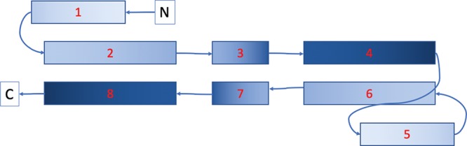
Schematic drawing of the SYCE1 construct with each box corresponding to one predicted α-helix. The SYCE sequence of approximately 120 amino acids corresponding to helices 1–4 is duplicated and linked by a tether to a repeat of the same sequence comprised of helices 5–8.

Deriving the Models

Based on the sequence and secondary structure predictions (a combination of those of RaptorX⁴⁷ and HHpred⁴⁸), 40 initial configurations were generated using the CB algorithm. An example is shown in Figure 15a along with its hydration layer; its scattering curve is compared to the experimental data (from ref (24)) in Figure 15b. As shown, the fitting is limited to the domain q ∈ [0, 0.3] Å^–1, which balances the twin considerations of a sufficient resolution and reliable signal-to-noise ratio. Using Monte Carlo optimization, the structure is altered until a reliable fit χ_f² + χ_nl + χ_con < 0.008 is obtained, where the potential χ_con is based on the contact predictions described above. One such model is shown in Figure 15c along with its scattering curve in Figure 15d. The identical chains of the structure have folded to lie (nearly) parallel with the end termini occupying a local neighborhood. Two example models for which χ_f² + χ_nl + χ_con < 0.008 are shown in Figure 16a,b. Panels c and d of Figure 16 indicate one of the coiled-coil structures and depict the pairwise distances associated with the contact prediction terms χ_con. All models share the elongated bend shape with a antiparallel coiled-coil arrangement of helix 2–4 to helix 6–8, respectively. The first helix in each helix (helices 1 and 5, respectively) show different orientations which reflect the expected conformational flexibility of the protein in solution. Importantly, the central coiled coil (made of helices 3 and 7, respectively) is not based on the constraints given a priori but is entirely based on the optimization against the experimental data. Although a bead model results in a similar overall shape,²⁴ our method is able to derive a more detailed molecular model with distinct structural features such as the central coiled coil.

Figure 15.

Illustrations of the optimization process used to obtain the model predictions for structural core of human SYCE1. (a) Initial starting configuration of the backbone based only on the sequence data shown in Figure 14. Also shown as spheres are the molecules of the hydration layer. Large black and white spheres indicate the end termini. (b) Scattering curve of the initial configuration (blue) overlaid on the scattering data (red). (c) Model prediction for which χ_f² + χ_nl + χ_con < 0.008; the end termini are next to each other. (d) Final scattering curve compared to experimental data.

Figure 16.

Illustrations of the model predictions. (a, b) All model predictions. (c) One of the coiled-coil units of (a) with black tubes representing the contact prediction distances, as seen along the axis of the unit. (d) Tilted helical structure of the coiled-coil unit. (e) Model obtained by minimizing the chi-squared measure χ_nl + χ_con only (i.e., without taking the scattering data into account).

Experimental Scattering Data Is Crucial to the Prediction Quality

One might ask if the contact predictions alone were sufficient to predict the structure, since they are crucial to forming (some of) the coiled-coil structure. To test this, we derived models by minimizing the chi-squared measure χ_nl + χ_con (i.e., ignoring the scattering data); a typical example is shown in Figure 16e. The outer α-helices are present as the contact prediction constraint χ_con forces these structures to form. However, the whole structure is significantly folded. This folding was found to be a typical property of models obtained by minimizing only χ_nl + χ_con, and the degree of folding was far from consistent. The clear effect of further enforcing the model fit the scattering data is twofold: first straightening out the whole structure and second, in doing so, developing a coiled-coil geometry in the middle of the structure.

Fitting to the Scattering Data and Contact Predictions Is Not Straightforward

As a final note, we note that of the 40 initial structures generated, only 5 obtained a suitably low combined chi-squared statistic (χ_f² + χ_nl + χ_con < 0.008). All five structures, two of which are shown in Figure 16, were basically identical in this case (comparative values > 0.9), so there was no need for any post hoc structural comparison analysis. By comparison all 40 lead to models for which χ_nl + χ_con < 0.008. As we have just seen, there is significant value in the extra information provided by the scattering data. The difficulty with obtaining suitable fits indicates that in the future more advanced optimization techniques than a straightforward Monte Carlo search may be needed.

Discussion

Summary of Results

This paper describes in-depth the development of a tertiary structure model for BioSAXS data interpretation. A number of key points have been demonstrated with regard to its potential use for the structural biology community. First, if the method starts with a known structure with a similar tertiary structure to the target structure, e.g., a homology model or an incomplete (core) model for a structure, then it will likely find a highly accurate fit to the presumably correct structure, as verified on a benchmark set of proteins. Second, given a near-complete absence of tertiary structural information, save that available from sequence data such as secondary structure predictions, the technique can generate realistic representations of the structure’s fold. Further, in this ab initio scenario there is the potential to reliably separate realistic predictions from those which are not biologically plausible, by both constraining the fitting procedure and applying optimization filtering. This final result, demonstrated here on lysozyme, is a significant result; there exists no purely ab initio SAXS technique so far which has achieved such detailed predictions of the protein’s fold (a number of techniques superimpose tertiary and secondary structures into ab initio bead predictions but this requires extra information such as a valid homologous structure). We now discuss various aspects of the predictions and compare them to existing methods.

Data Requirements

The fundamental information required to construct the backbone model is the sequence, used to identify secondary structures (linker, strand, and α-helix). This information can be obtained from the sequence using, for example, the publicly available jPred server.⁴⁹ Then we only need the scattering data to fit this model to. Therefore, in its most basic form the algorithm can yield predictions from only two files: a sequence file and a scattering data file.

We can also use the sequence file and existing spatial information to constrain the potential search space. In the case of the lysozyme predictions, the search space was additionally constrained using contact predictions. Contact predictions can be obtained based on the sequence using, for example, the RaptorX server. The server does include homology model generation if applicable, but we have only used the list of amino acid pairs which have a high sequence correlation. As discussed above, we constrain their mutual distance. Similarly, the SYCE1 protein models were additionally constrained using coiled-coil sequence alignments, as discussed under Results.

The technique can also accommodate the use of additional information; for example, PDB files could be used as initial homology models or partial structure specifications. In this case the necessary pieces information required are the secondary structure specifications and the C^α coordinates. In general, any additional information used to constrain the search space needs to provide information on the C^α coordinates, in particular what secondary structure type is it, and how does its constrain its spatial coordinates (i.e., a fixed location or a fixed distances for pairs of C^α coordinates)? It is possible, for example, to fix the coordinates of a subsection of the target structure and only vary the rest, if a partial prediction is already present.

Comparisons to Existing Techniques

With regard to comparisons to existing techniques there are two categories to be discussed. The first is the set of different experimental methods used to derive structures in the Protein Data Bank. The predictions from our methods, applied to small angle scattering data, can be near this level of quality if a reliable initial structural model is provided. This was demonstrated under Results when we used PDB structures as a starting model; the algorithm yielded structures with RMSD measures (by comparison to the PDB structure) highly comparable to experimentally obtained models (for α-carbon positions). In a purely ab initio scenario our results indicate it is currently difficult to obtain this level of accuracy on a reliable basis (although one can get single angstrom RMSD measures). However, as shown in Figure 13d, there is some indication that, if extra constraints such as contact predictions from homologous sequences can be enforced to a high degree of accuracy, there is the potential to reach similar levels of structural resolution to these alternative experimental techniques.

Ab Initio Methods

The second comparison would be to SAXS-specific ab initio techniques for interpreting BioSAXS data. These include the bead based models such as GASBOR and DAMMIN.^13,50 However, a direct comparison is difficult because the natures of predictions are different. Neither method makes explicit predictions of the sequence-ordered tertiary structure of the molecule. Both are composed of effective scattering beads. The DAMMIN model aims to predict the volume occupied by the molecule by creating a cloud of beads, while GASBOR aims for a structure with a chainlike nature constraining bead–bead distances, but there is no explicit secondary structure in the model. However, previously a technique for comparing bead models to tertiary structures was suggested, using a measurement, the normalized spatial discrepancy (NSD), derived from several metrics for comparing the distributional similarity of two sets of points.⁵¹ This calculation is implemented in the SUPCOMB routines, part of the ATSAS package. The SUPCOMB algorithm rotates (and translates) the bead clouds to minimize their NSD measure, as described in ref (51). This does not account for the sequential nature of the chain in the models derived here. Instead, it in effect measures the similarity of two point clouds, but it is a sensible means of comparing the results of the results obtained in this study to GASBOR predictions (the closest to the CB model in that it develops chainlike structures). We compared the GASBOR prediction for lysozyme (obtained from SASBDB,⁴⁵ code SASDAG2) for the same scattering data that was used in Results to obtain the CB algorithm prediction; note that both use the same q domain ([0, 0.4] Å^–1). In both cases the structures were compared to the 1LYZ structure via their NSD measures. An NSD value below 1 is generally considered a good match.⁵² A small subset of the results are indicated in Table 1; all values are below 1. The quality of this fit is illustrated in Figure 17, where the predictions are superimposed on the solvent-accessible surface area of the 1LYZ structure. Therefore, in terms of point cloud comparison, both prediction techniques can yield very similar predictions. This is not such a surprise as both fit the low q portion of the scattering curve, which contains the large scale structural information, very well.

Table 1. Various Structural Comparison Metrics for Predictions of Lysozyme Predictions, All by Comparison to the 1LYZ Structure and All Quoted to Three Significant Figures.

prediction type	SUPCOMB NSD		RMSD
GASBOR model	0.813	N/A	N/A
CB pred 1	0.880	0.729	9.77
CB pred 2	0.863	0.703	9.22
CB pred 3	0.889	0.708	10.3
CB pred 4	0.866	0.133	13.2

Figure 17.

GASBOR (obtained from SASBDB, code SASDAG2) and CB algorithm models for lysozyme superimposed on the 1LYZ crystal structure. (a) Bead cloud (red) of a GASBOR prediction for the same lysozyme scattering data as used above, obtained from SASBDB (code SASDAG2). A lysozyme prediction (blue curve) from Results for which the SUPCOMB NSD is 0.813 and knot fingerprint statistic (both by comparison to the 1LYZ PDB structure). (c) Lysozyme prediction (green curve) from Results for which the SUPCOMB NSD is 0.8664 and knot fingerprint statistic (both by comparison to the 1LYZ PDB structure). (d) Secondary structure sections 1–10 of the CB lysozyme model shown in (c).

What is of particular interest is that structures with significantly different knot fingerprint statistics yield very similar SUPCOMB and similar RMSD measures. Two examples of CB predictions are shown in Figure 17, panels b and c, respectively: and . Both structures fit very well inside the lysozyme solvent accessible surface area, as indicated by the near identical NSD measures. The low measure of the structure in Figure 17c is seen in Figure 17d to be a result of the fact that the subsection involving the strand structure has a significantly different subfold compared to the PDB structure, shown in Figure 12b. In particular, the β-sheet structure “folds back” in the direction opposite to that of the PDB structure (and the high structure shown in Figure 12c). This highlights the benefit of the additional predictive information provided directly by the CB algorithm: one can discern geometrically distinct predictions and thus make a more precise prediction about the structure of the protein under consideration.

The ATSAS package does allow for the interpretation of bead models with tertiary structure through the use of the CORAL package.⁵⁰ The package attempts to fit a structure into the bead model with a mixture of known (manually assigned) and unknown secondary structure elements. This procedure was performed in ref (24) to provide evidence that the SYCE1 core modeled in ref (24) was a coiled-coil domain; a rendering of this model is shown in Figure 18a. Two coiled coils were superimposed on a bead model with CORAL providing an additional linker section to join them. Our model simply uses the sequence data to determine the secondary structural elements; then it is able to try millions of differing (physically realistic) folds and tests each time if they satisfy the scattering data, a much more direct and exhaustive test, which relies on far less user input. What is interesting is that this technique predicts an additional coiled-coil domain at the structure’s center (cf. panels a and b of Figure 18), owing to the sequence interpretation splitting of the helical units. The method presented in this paper offers more flexibility in terms of using additional structural constraints and is more amenable to automated structural evaluation. Its main comparative advantage, over the coral package, is the potentially exhaustive automated search of a space of potential tertiary folds with realistically constrained secondary structure.

Figure 18.

Comparison of the CORAL derived model of the SYCE1 core obtained in ref (24) (a) and an example CB derived model (b).

Computation Time

A single calculation comprising the CB algorithm, the generation of the hydration layer, and calculation of the scattering curve takes on the order of 0.05 s for lysozyme (129 residues) and 0.5 s for BSA (433 residues), both based on calculations performed on a single CPU, with the main cost coming from the Debye formula, eq 5. As far as the actual optimization goes, the timing can vary significantly; this depends on the number of secondary units which can be changed, the randomized initial condition, and the difficulty in satisfying additional restrictions such as the contact predictions (and how tightly they have been penalized). The ab initio lysozyme predictions generally varied between 10 min and 1 h. For the SYCE1 chain (318 residues) it was closer to 20 h (that said, as mentioned above the predictions produced in this case were reliably accurate). In future we will look to implement Bayesian learning techniques for the search, as a large number of models suggested by the Monte Carlo sampling overlap themselves and consistently trying such models wastes much time. This will be crucial to ensuring it can be run for larger molecules in the future.

Number of Initial Models

One might ask how many predictions are required in order to obtain a viable structure (ab initio). The examples here present a contrasting picture. The lysozyme cases consistently produced structure which fit the scattering data, but as discussed only a relatively small percentage (about 8%) were considered a sufficiently good fit to the scattering data (i.e., a sufficiently low RMSD with respect to the PDB structure and high value). By contrast, from 40 initial conditions for the SYCE1 molecule only 12.5% were able to fit the scattering data, but all were nearly identical () and excellent candidate structures. It is likely this is because lysozyme is a globular protein while SYCE1 has a very flat, linear structure. It is relatively easy to distort our model into a globular shape, but it allows for more structural variance, while the more linear structure is harder to form but much more constrained. The consistent evidence is that, currently, one might need at least 10 optimization runs in order to obtain a good quality prediction. A future aim will be to better enforce contact predictions or other constraints during the fitting procedure in order to bring down this ratio.

Conclusion

As a solution-based technique, BioSAXS can provide structural information for targets where crystallization and cryo-electron microscopic (cryo-EM) techniques are challenging. Also, the method allows data collection in a more natural environment than techniques such as crystallography and cryo-EM. Additionally, SAXS is not limited by protein size, as is the case for cryo-EM and NMR. Therefore, there is a clear need to develop the techniques for interpretation of this data in an ab initio setting which improve on the levels of structural detail provided by the bead models currently popular.

In this paper we have shown that curve representation with hydration shell provides a molecular model for BioSAXS data with fits as good as or better than traditional bead and envelope models. Unlike these models our model includes a complete secondary and tertiary model description. Importantly, starting from random models that only take secondary structure information and sequence-dependent distance constraints into account, a physically meaningful 3D model can be obtained by fitting models against the experimental data. That this is possible is due to the fact that the model is described with far fewer parameters compared to even a coarse-grained model that required three coordinates for each amino acid, combined with use of geometric constraints for regular secondary structural elements.

In order to show the potential of this ab initio technique, it was applied to a tethered core component of the human SYCE1 protein, for which no high resolution structural data is available. The model derived was based on sequence information alone and matches that of a model that was previously reported in ref (24), where the model was based on manual inspection of the sequences coupled with the fitting of ideal coiled coil segments to experimental scattering data. Importantly, while the previously modeled structure includes two coiled coil segments, the model derived here recognized that this was the minimum number of segments required to explain the curved structure and that the true structure could consist of multiple coiled coils interrupted by short linkers. Thus, our novel ab initio method has successfully generated a highly plausible model from experimental scattering data without the need for any more than minimal manual evaluation. This facility will be crucial for ab initio structural determination (from BioSAXS data) of larger molecules where it would not be practical to generate structures manually.

Further experimental information such as distance information from any other source can easily been added in the form of additional restraints into the optimization algorithm. The model’s explicit description of realistic secondary structure means additional information, such as contact predictions, radius of gyration, hydrophobicity of the chain, and disulfide bonding, can be employed as model constraints in the future. This will further enhance the accuracy of all potential models, and in particular help the end user to distinguish mathematically correct but physically less likely models from correct solution. The secondary knot fingerprint statistic developed shows significant potential to evaluate structural similarities of models and hence to further automate this vital validation step.

The two future next steps are (i) the application of this method to multimeric structures where each known monomer structure can initially be treated as rigid body and then refined in order to account for local changes in solution and (ii) the application to larger, de novo structures where the exact 3D structure remains elusive. The second goal will require further refinements of the search space method of the optimization algorithm. The application to homomultimers is straightforward and requires only minor addition to the existing code; we expect this to be the major initial application of our methods. Due to the limited information content of small angle X-ray scattering data, the ab initio fold determination will depend on the accuracy of secondary structure prediction combined with appropriately weighted distance constraints such as those discussed above.

Supporting Information Available

The Supporting Information is available free of charge at https://pubs.acs.org/doi/10.1021/acs.jctc.9b01010.

• Additional deatails on the model’s construction and testing (PDF)

Financial support from the Biophysical Sciences Institute and the Addison-Wheeler fellowship for C.P. is gratefully acknowledged.

The authors declare no competing financial interest.

References

- Petoukhov M. V.; Svergun D. I. Applications of small-angle X-ray scattering to biomacromolecular solutions. Int. J. Biochem. Cell Biol. 2013, 45, 429–437. 10.1016/j.biocel.2012.10.017. [DOI] [PubMed] [Google Scholar]
- Kikhney A. G.; Svergun D. I. A practical guide to small angle X-ray scattering (SAXS) of flexible and intrinsically disordered proteins. FEBS Lett. 2015, 589, 2570–2577. 10.1016/j.febslet.2015.08.027. [DOI] [PubMed] [Google Scholar]
- Mina J. G.; Thye J. K.; Alqaisi A. Q.; Bird L. E.; Dods R. H.; Grøftehauge M. K.; Mosely J. A.; Pratt S.; Shams-Eldin H.; Schwarz R. T.; Pohl E.; Denny P. W. Functional and phylogenetic evidence of a bacterial origin for the first enzyme in sphingolipid biosynthesis in a phylum of eukaryotic protozoan parasites. J. Biol. Chem. 2017, 292, 12208–12219. 10.1074/jbc.M117.792374. [DOI] [PMC free article] [PubMed] [Google Scholar]
- Svergun D. I.; Koch M. H.; Timmins P. A.; May R. P.. Small Angle X-ray and Neutron Scattering from Solutions of Biological Macromolecules; Oxford University Press: 2013; Vol. 19. [Google Scholar]
- Rambo R. P.; Tainer J. A. Bridging the solution divide: comprehensive structural analyses of dynamic RNA, DNA, and protein assemblies by small-angle X-ray scattering. Curr. Opin. Struct. Biol. 2010, 20, 128–137. 10.1016/j.sbi.2009.12.015. [DOI] [PMC free article] [PubMed] [Google Scholar]
- Svergun D.; Barberato C.; Koch M. H. CRYSOL–a program to evaluate X-ray solution scattering of biological macromolecules from atomic coordinates. J. Appl. Crystallogr. 1995, 28, 768–773. 10.1107/S0021889895007047. [DOI] [Google Scholar]
- Schneidman-Duhovny D.; Hammel M.; Sali A. FoXS: a web server for rapid computation and fitting of SAXS profiles. Nucleic Acids Res. 2010, 38, W540–W544. 10.1093/nar/gkq461. [DOI] [PMC free article] [PubMed] [Google Scholar]
- Poitevin F.; Orland H.; Doniach S.; Koehl P.; Delarue M. AquaSAXS: a web server for computation and fitting of SAXS profiles with non-uniformally hydrated atomic models. Nucleic Acids Res. 2011, 39, W184–W189. 10.1093/nar/gkr430. [DOI] [PMC free article] [PubMed] [Google Scholar]
- Wright D. W.; Perkins S. J. SCT: a suite of programs for comparing atomistic models with small-angle scattering data. J. Appl. Crystallogr. 2015, 48, 953–961. 10.1107/S1600576715007062. [DOI] [PMC free article] [PubMed] [Google Scholar]
- Perkins S. J.; et al. Atomistic modelling of scattering data in the Collaborative Computational Project for Small Angle Scattering (CCP-SAS). J. Appl. Crystallogr. 2016, 49, 1861–1875. 10.1107/S160057671601517X. [DOI] [PMC free article] [PubMed] [Google Scholar]
- Schneidman-Duhovny D.; Hammel M.; Tainer J. A.; Sali A. FoXS, FoXSDock and MultiFoXS: Single-state and multi-state structural modeling of proteins and their complexes based on SAXS profiles. Nucleic Acids Res. 2016, 44, W424–W429. 10.1093/nar/gkw389. [DOI] [PMC free article] [PubMed] [Google Scholar]
- Franke D.; Svergun D. I. DAMMIF, a program for rapid ab-initio shape determination in small-angle scattering. J. Appl. Crystallogr. 2009, 42, 342–346. 10.1107/S0021889809000338. [DOI] [PMC free article] [PubMed] [Google Scholar]
- Svergun D. I.; Petoukhov M. V.; Koch M. H. Determination of domain structure of proteins from X-ray solution scattering. Biophys. J. 2001, 80, 2946–2953. 10.1016/S0006-3495(01)76260-1. [DOI] [PMC free article] [PubMed] [Google Scholar]
- Hausrath A.; Goriely A. Continuous representations of proteins: Construction of coordinate models from curvature profiles. J. Struct. Biol. 2007, 158, 267–281. 10.1016/j.jsb.2006.11.003. [DOI] [PubMed] [Google Scholar]
- Lundgren M.; Krokhotin A.; Niemi A. J. Topology and structural self-organization in folded proteins. Phys. Rev. E 2013, 88, 042709. 10.1103/PhysRevE.88.042709. [DOI] [PubMed] [Google Scholar]
- Kneller G. R.; Hinsen K. Protein secondary-structure description with a coarse-grained model. Acta Crystallogr., Sect. D: Biol. Crystallogr. 2015, 71, 1411–1422. 10.1107/S1399004715007191. [DOI] [PubMed] [Google Scholar]
- Ramachandran G. N.; Ramakrishnan C.; Sasisekharan V. Stereochemistry of polypeptide chain configurations. J. Mol. Biol. 1963, 7, 95–99. 10.1016/S0022-2836(63)80023-6. [DOI] [PubMed] [Google Scholar]
- Bolcun-Filas E.; Speed R.; Taggart M.; Grey C.; de Massy B.; Benavente R.; Cooke H. J. Mutation of the mouse Syce1 gene disrupts synapsis and suggests a link between synaptonemal complex structural components and DNA repair. PLoS Genet. 2009, 5, e1000393. 10.1371/journal.pgen.1000393. [DOI] [PMC free article] [PubMed] [Google Scholar]
- Costa Y. e. a. Two novel proteins recruited by synaptonemal complex protein 1 (SYCP1) are at the centre of meiosis. J. Cell Sci. 2005, 118, 2755–2762. 10.1242/jcs.02402. [DOI] [PubMed] [Google Scholar]
- Park H. H. X-ray crystallographic studies of the middle part of the human synaptonemal complex protein 1 coiled-coil domain. Acta Crystallogr., Sect. F: Struct. Biol. Commun. 2015, 71, 1131–1134. 10.1107/S2053230X15012728. [DOI] [PMC free article] [PubMed] [Google Scholar]
- Davies O. R.; Maman J. D.; Pellegrini L. Structural analysis of the human SYCE2–TEX12 complex provides molecular insights into synaptonemal complex assembly. Open Biol. 2012, 2, 120099. 10.1098/rsob.120099. [DOI] [PMC free article] [PubMed] [Google Scholar]
- Syrjänen J. L.; Pellegrini L.; Davies O. R. A molecular model for the role of SYCP3 in meiotic chromosome organisation. eLife 2014, 3, e02963. 10.7554/eLife.02963. [DOI] [PMC free article] [PubMed] [Google Scholar]
- Dunce J. M.; Dunne O. M.; Ratcliff M.; Millán C.; Madgwick S.; Usón I.; Davies O. R. Structural basis of meiotic chromosome synapsis through SYCP1 self-assembly. Nat. Struct. Mol. Biol. 2018, 25, 557–569. 10.1038/s41594-018-0078-9. [DOI] [PMC free article] [PubMed] [Google Scholar]
- Dunne O. M.; Davies O. R. Molecular structure of human synaptonemal complex protein SYCE1. Chromosoma 2019, 128, 223–236. 10.1007/s00412-018-00688-z. [DOI] [PMC free article] [PubMed] [Google Scholar]
- Carroll D.; Hankins E.; Kose E.; Sterling I. A survey of the differential geometry of discrete curves. Mathematical Intelligencer 2014, 36, 28–35. 10.1007/s00283-014-9472-2. [DOI] [Google Scholar]
- Majorek K. A.; Porebski P. J.; Dayal A.; Zimmerman M. D.; Jablonska K.; Stewart A. J.; Chruszcz M.; Minor W. Structural and immunologic characterization of bovine, horse, and rabbit serum albumins. Mol. Immunol. 2012, 52, 174–182. 10.1016/j.molimm.2012.05.011. [DOI] [PMC free article] [PubMed] [Google Scholar]
- Wand M. P.; Jones M. C.. Kernel Smoothing; CRC Press: 1994. [Google Scholar]
- Putnam C. D.; Hammel M.; Hura G. L.; Tainer J. A. X-ray solution scattering (SAXS) combined with crystallography and computation: defining accurate macromolecular structures, conformations and assemblies in solution. Q. Rev. Biophys. 2007, 40, 191–285. 10.1017/S0033583507004635. [DOI] [PubMed] [Google Scholar]
- Elias M.; Wellner A.; Goldin-Azulay K.; Chabriere E.; Vorholt J. A.; Erb T. J.; Tawfik D. S. The molecular basis of phosphate discrimination in arsenate-rich environments. Nature 2012, 491, 134. 10.1038/nature11517. [DOI] [PubMed] [Google Scholar]
- Debye P. Zerstreuung von röntgenstrahlen. Ann. Phys. 1915, 351, 809–823. 10.1002/andp.19153510606. [DOI] [Google Scholar]
- Brown P.; Fox A.; Maslen E.; O’Keefe M.; Willis B.. International Tables for Crystallography Vol. C: Mathematical, Physical and Chemical Tables; Springer: 2006; pp 554–595. [Google Scholar]
- Kleywegt G. J.; Jones T. A. Databases in protein crystallography. Acta Crystallogr., Sect. D: Biol. Crystallogr. 1998, 54, 1119–1131. 10.1107/S0907444998007100. [DOI] [PubMed] [Google Scholar]
- Fraser R.; MacRae T.; Suzuki E. An improved method for calculating the contribution of solvent to the X-ray diffraction pattern of biological molecules. J. Appl. Crystallogr. 1978, 11, 693–694. 10.1107/S0021889878014296. [DOI] [Google Scholar]
- Schwartz R.; Istrail S.; King J. Frequencies of amino acid strings in globular protein sequences indicate suppression of blocks of consecutive hydrophobic residues. Protein Sci. 2001, 10, 1023–1031. 10.1110/ps.33201. [DOI] [PMC free article] [PubMed] [Google Scholar]
- Kufareva I.; Abagyan R.. Homology Modeling; Springer: 2011; pp 231–257. [Google Scholar]
- Zemla A.; Venclovas Č.; Moult J.; Fidelis K. Processing and evaluation of predictions in CASP4. Proteins: Struct., Funct., Genet. 2001, 45, 13–21. 10.1002/prot.10052. [DOI] [PubMed] [Google Scholar]
- Millett K. C.; Rawdon E. J.; Stasiak A.; Sułkowska J. I. Identifying knots in proteins. Biochem. Soc. Trans. 2013, 41, 533–537. 10.1042/BST20120339. [DOI] [PubMed] [Google Scholar]
- Tubiana L.; Orlandini E.; Micheletti C. Probing the entanglement and locating knots in ring polymers: a comparative study of different arc closure schemes. Prog. Theor. Phys. Suppl. 2011, 191, 192–204. 10.1143/PTPS.191.192. [DOI] [Google Scholar]
- Jamroz M.; Niemyska W.; Rawdon E. J.; Stasiak A.; Millett K. C.; Sułkowski P.; Sulkowska J. I. KnotProt: a database of proteins with knots and slipknots. Nucleic Acids Res. 2015, 43, D306–D314. 10.1093/nar/gku1059. [DOI] [PMC free article] [PubMed] [Google Scholar]
- Sułkowska J. I.; Rawdon E. J.; Millett K. C.; Onuchic J. N.; Stasiak A. Conservation of complex knotting and slipknotting patterns in proteins. Proc. Natl. Acad. Sci. U. S. A. 2012, 109, E1715–E1723. 10.1073/pnas.1205918109. [DOI] [PMC free article] [PubMed] [Google Scholar]
- Diamond R. Real-space refinement of the structure of hen egg-white lysozyme. J. Mol. Biol. 1974, 82, 371–391. 10.1016/0022-2836(74)90598-1. [DOI] [PubMed] [Google Scholar]
- Rolfsen D.Knots and Links; American Mathematical Society: 2003; Vol. 346. [Google Scholar]
- Rambo R. P.; Tainer J. A. Accurate assessment of mass, models and resolution by small-angle scattering. Nature 2013, 496, 477. 10.1038/nature12070. [DOI] [PMC free article] [PubMed] [Google Scholar]
- Schneidman-Duhovny D.; Hammel M.; Tainer J. A.; Sali A. Accurate SAXS profile computation and its assessment by contrast variation experiments. Biophys. J. 2013, 105, 962–974. 10.1016/j.bpj.2013.07.020. [DOI] [PMC free article] [PubMed] [Google Scholar]
- Valentini E.; Kikhney A. G.; Previtali G.; Jeffries C. M.; Svergun D. I. SASBDB, a repository for biological small-angle scattering data. Nucleic Acids Res. 2015, 43, D357–D363. 10.1093/nar/gku1047. [DOI] [PMC free article] [PubMed] [Google Scholar]
- Cock P. J. A.; Antao T.; Chang J. T.; Chapman B. A.; Cox C. J.; Dalke A.; Friedberg I.; Hamelryck T.; Kauff F.; Wilczynski B.; de Hoon M. J. L. Biopython: freely available Python tools for computational molecular biology and bioinformatics. Bioinformatics 2009, 25, 1422–1423. 10.1093/bioinformatics/btp163. [DOI] [PMC free article] [PubMed] [Google Scholar]
- Peng J.; Xu J. RaptorX: exploiting structure information for protein alignment by statistical inference. Proteins: Struct., Funct., Genet. 2011, 79, 161–171. 10.1002/prot.23175. [DOI] [PMC free article] [PubMed] [Google Scholar]
- Zimmermann L.; Stephens A.; Nam S.-Z.; Rau D.; Kübler J.; Lozajic M.; Gabler F.; Söding J.; Lupas A. N.; Alva V. A completely reimplemented MPI bioinformatics toolkit with a new HHpred server at its core. J. Mol. Biol. 2018, 430, 2237–2243. 10.1016/j.jmb.2017.12.007. [DOI] [PubMed] [Google Scholar]
- Drozdetskiy A.; Cole C.; Procter J.; Barton G. J. JPred4: a protein secondary structure prediction server. Nucleic Acids Res. 2015, 43, W389–W394. 10.1093/nar/gkv332. [DOI] [PMC free article] [PubMed] [Google Scholar]
- Petoukhov M. V.; Franke D.; Shkumatov A. V.; Tria G.; Kikhney A. G.; Gajda M.; Gorba C.; Mertens H. D.; Konarev P. V.; Svergun D. I. New developments in the ATSAS program package for small-angle scattering data analysis. J. Appl. Crystallogr. 2012, 45, 342–350. 10.1107/S0021889812007662. [DOI] [PMC free article] [PubMed] [Google Scholar]
- Kozin M. B.; Svergun D. I. Automated matching of high-and low-resolution structural models. J. Appl. Crystallogr. 2001, 34, 33–41. 10.1107/S0021889800014126. [DOI] [Google Scholar]
- Konarev P. V.; Petoukhov M. V.; Svergun D. I. Rapid automated superposition of shapes and macromolecular models using spherical harmonics. J. Appl. Crystallogr. 2016, 49, 953–960. 10.1107/S1600576716005793. [DOI] [PMC free article] [PubMed] [Google Scholar]
Associated Data
This section collects any data citations, data availability statements, or supplementary materials included in this article.