High-resolution 4-D acquisition of freely swimming human sperm cells without staining

We present a new high-resolution stain-free imaging method for optical CT of individual sperm cells during free swim.

Abstract

We present a new acquisition method that enables high-resolution, fine-detail full reconstruction of the three-dimensional movement and structure of individual human sperm cells swimming freely. We achieve both retrieval of the three-dimensional refractive-index profile of the sperm head, revealing its fine internal organelles and time-varying orientation, and the detailed four-dimensional localization of the thin, highly-dynamic flagellum of the sperm cell. Live human sperm cells were acquired during free swim using a high-speed off-axis holographic system that does not require any moving elements or cell staining. The reconstruction is based solely on the natural movement of the sperm cell and a novel set of algorithms, enabling the detailed four-dimensional recovery. Using this refractive-index imaging approach, we believe that we have detected an area in the cell that is attributed to the centriole. This method has great potential for both biological assays and clinical use of intact sperm cells.

INTRODUCTION

In intracytoplasmic sperm injection (ICSI), a single sperm is selected for direct injection into the ovum. This process poses an innate difficulty, as the natural sperm selection induced by the race to the ovum, perfected by millions of years of evolution, is replaced by a selection performed by a clinician (1). Today, clinicians base the process of sperm selection on morphology and dynamics assessment, which is carried out using two-dimensional (2-D) imaging methods, such as bright-field microscopy (BFM), differential interference contrast (DIC) microscopy, Hoffman’s microscopy, and Zernike’s phase-contrast microscopy (2, 3). These imaging methods lack quantitative contrast, because of the prohibition of using exogenous contrast agents in human ICSI, and have distinctive imaging artifacts. Moreover, both the structure and the natural movement of the human sperm cell are three-dimensional (3-D); thus, an entire aspect of the dynamics and morphology of sperm cells is currently disregarded because of technological barriers. Holographic imaging allows for a fully quantitative measurement of the cell optical thickness [i.e., the product of the refractive index (RI) and the physical thickness] (4). This enables the stain-free examination of the sperm based not only on the 2-D morphology of the cell head but also on optical thickness–based parameters, such as dry mass, and phase volume (5, 6).

In addition to head morphology, sperm flagellum defects have been postulated to be prognostic for fertilization failure (7). However, the complex shape and motion of the flagellum is typically disregarded in sperm selection protocols because of its low visibility and 3-D nature (1). Most commonly, four-dimensional (4-D) tracking methods for sperm cells have been suggested on the basis of pinpointing the 3-D location of a single point on the sperm, usually the sperm head centroid, over time (4, 8–11). Corkidi et al. (8) suggested such a method, with a system based on a piezoelectric device displacing a large focal distance objective mounted on a microscope to acquire dozens of image stacks per second, where each stack of images spans across a depth of 100 μm. However, in this previous work, sperm trajectories were obtained manually as the main focus was the high-speed acquisition of 3-D data, thus making it inappropriate for clinical use. Su et al. (9) suggested an automated, high-throughput tracking method based on holographic lens-free shadows of sperm cells that are simultaneously acquired at two different wavelengths, emanating from two sources placed at 45° with respect to each other, where the 3-D location of each sperm is determined by the centroids of its head images reconstructed in the vertical and oblique channels. Digital holographic microscopy images have also been previously used to track sperm cell trajectories by using wavefront propagation to obtain multiple focus planes and then applying either Tamura’s coefficient (10), a criterion based on the invariance of both energy and amplitude (11), or a criterion based on the steepest intensity gradient along the z axis (12), to estimate the in-focus distance.

In the past couple of years, several studies aimed at tracking the location of the entire flagellum in 3-D space and time (13–15). Silva-Villalobos et al. (13) used an oscillating objective mounted in a bright-field optical microscope, covering a 16-μm depth at a rate of 5000 images per second, where the best flagellum-focused subregions were associated to their respective z positions. Bukatin et al. (14) developed an algorithm that reconstructs the vertical beat component from 2-D BFM images by first identifying the projected 2-D shape of the flagellum based on the pixel intensity levels and then estimating the z coordinate by analyzing the intensity profile along cross sections normal to the flagellum in the image plane, exploiting the fact that the width of the halo is correlated to the z displacement from the focus plane. Last, Daloglu et al. (15) recently extended their former work using simultaneous illumination from two sources emerging from two oblique angles (9), reporting a high-throughput and label-free holographic method that can simultaneously reconstruct both the full beating pattern of the flagellum and the translation and spin of the head. These methods evaluate the trajectories of the sperm in space but do not address the problem of reconstructing the 3-D morphology of the head, which contains clinically important organelles, preventing full 4-D morphological evaluation.

Label-based confocal fluorescence microscopy can obtain high spatial-resolution 3-D cell imaging (16). However, it cannot be used in human sperm cell selection during ICSI as staining is not allowed. Furthermore, even when using label-based confocal fluorescence microscopy for live cells in animal fertilizations or in biological studies, it is very challenging to obtain the entire sperm head and flagellum 3-D reconstruction during rapid free swim because of the need to scan over time and the low amounts of fluorescence emission in each temporal frame. The gross surface morphology of the bovine sperm head was previously reconstructed without staining by using a Gaussian beam inducing self-rotation of the cell and the shape from silhouette algorithm (17). This method, however, could not capture the internal organelles of the sperm head or its 4-D flagellum beating. In tomographic phase microscopy, interferometric projections of the specimen taken from multiple angles are processed and positioned in the 3-D Fourier space so that the RI map can be reconstructed. Recently, a commercial tomographic microscope was used to recover the 3-D RI distributions of animal (nonhuman) sperm cells (18). Yet, this method scans only 30 illumination angles and at a limited angular range; thus, it is unable to fully image freely swimming sperm cells. Thus, the problem of reconstructing the 3-D dynamic morphologies of uninterrupted swimming sperm cell heads has not yet been solved. Here, we present the first 4-D acquisition method for the entire sperm (head with organelles and flagellum) during free swim and without staining.

RESULTS

Our method is based on rapid quantitative phase microscopy and a novel set of reconstruction algorithms providing the highly detailed 4-D distribution of the sperm cell during swim. Holographic videos of sperm cells were acquired by off-axis holographic phase microscopy, which allows high-resolution complex wavefront acquisition from a single camera shot of dynamic sperm cells. The acquisition system contained an inverted microscope, equipped with a 100× oil-immersion objective, ×328 total magnification through the system, an external nearly-common-path interferometric module, and a fast digital camera, recording at 2000 frames/s (fps). Sperm cells swam freely in a perfusion chamber (see the “Optical setup for interferometric phase microscopy” section). We reconstruct the recorded sperm head and the flagellum individually, treating them as separate entities due to their physical dissimilarity, as described below.

Reconstructing the 3-D morphology of the sperm head

To recover the 3-D RI profile of the sperm head, we used a tomographic phase microscopy approach that takes into consideration diffraction effects. To position the processed projections in the 3-D Fourier space, it is essential to know the angle at which the projection of the object was captured. Existing tomographic approaches are based on either illumination rotation (18) or controlled sample rotation (19), allowing a priori knowledge on the angles of the acquired interferometric projections. Alternatively, random rotation of cells while flowing along a microfluidic channel or perfusion chamber can be used for tomography for a degenerate case, assuming rotation around a single axis (20, 21). In the case of a human sperm cell swimming freely, though, the swimming pattern is too complex to apply any of the existing tomographic algorithms as the algorithm must take into account the rotation around all three major axes: pitch, roll, and yaw. Modeling the sperm cell head as an ellipsoid, we were able to build a highly accurate algorithm for retrieving all three angles from each frame based on the minor and major radii extracted from the segmented phase maps of the head, requiring only a single acquisition per frame. This is done by extracting the three model constants (A, B, and C), illustrated in Fig. 1A, from the major and minor radii vectors, retrieved from hundreds of consecutive frames, while relying on the periodicity of sperm rolling. By virtue of the periodic swimming pattern, we obtain full (spiral) angular coverage for tomography, rather than the standard ±70° obtained in the illumination rotation method. Following this, each specific frame orientation is determined via interpolation, which is possible because of the basic asymmetry of the sperm cell, inducing A ≠ B ≠ C (see further details in the “head orientation recovery” section of Materials and Methods). Using this approach, we are able to recover the orientation that yields the same projected ellipse as the rotated ellipsoid model. Using continuity constraints, we are able to reliably limit the cases in which there is more than one orientation that causes the same projected ellipse and gain definitive recovery.

Fig. 1. Schematic illustrations for sperm cell head orientation recovery algorithm, where the camera plane is parallel to the x-y plane.

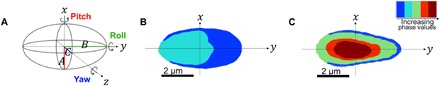
(A) 3-D ellipsoid model, including definition of the pitch, roll, and yaw angles, as well as the three model constants, A, B, and C. (B) The projection of a sperm cell head lying flat. (C) The projection of a sperm cell head lying on its side.

We then position the Rytov field of each projection at the calculated orientation in the 3-D Fourier space, allowing reconstruction of the 3-D RI distribution through optical diffraction tomography (ODT) theory (22). A representative result, obtained by applying our approach on 1000 recorded frames of a sperm swimming freely in a perfusion chamber, is given in Fig. 2. This result agrees with previous studies regarding the internal structure of the sperm cell head [e.g., (23)], clearly showing the three main components of the sperm head: cell membrane (light purple), acrosomal vesicle (yellow), and nucleus (red). Importantly, although we could not verify it experimentally, the sperm head reconstruction in Fig. 2 also reveals a higher-RI region in the proximal part of the head, closest to the midpiece, which may be attributed to the sperm centriole area [colored in dark purple in Fig. 2B]; this organelle, which is crucial for the development of the embryo after fertilization, has never been imaged before in live cells.

Fig. 2. A representative sperm cell head 3-D RI reconstruction from 1000 frames during free swim.

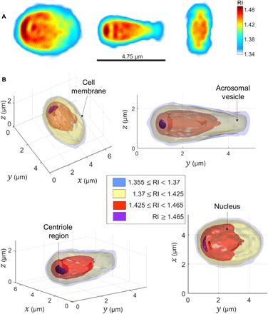
(A) Middle slices along the three main axes. Color bar denotes RI values. (B) Thresholded 3-D rendering from various perspectives. Two other cells are shown in fig. S5.

Validation of the ellipsoid model for sperm head orientation recovery

To confirm the validity of the ellipsoid model for sperm head orientation recovery, we took as inputs both the external 3-D shape of an actual sperm cell (fig. S1A) and its ellipsoid model (fig. S1B) and calculated the projections of each for the roll and pitch angles retrieved for each frame (fig. S2). Following this, we calculated the major and minor axis radii of each projection, as well as its orientation (i.e., native yaw angle). The results of this comparison are shown in fig. S3. Figure S3A shows the results obtained for the major radius from the projection of the actual sperm cell (cyan line) and the ellipsoid model (green circles) versus the original measurement from the holograms (blue asterisk). The mean absolute percentage (MAP) error between the result obtained from the actual sperm cell and the ellipsoid model is 2.73%. Figure S3B shows the results obtained for the minor radius from the projection of the actual sperm cell (cyan line) and the ellipsoid model (green circles) versus the original measurement from the holograms (blue asterisk). The MAP error between the result obtained from the sperm cell and ellipsoid model is 1.98% after removing the segmentation bias, indicating the nearly identical shape of all vectors. Last, fig. S3C shows the results obtained for the native yaw angle from the projection of the actual sperm cell (blue line) and ellipsoid model (red dashed line). These results demonstrate that this set of parameters is mapped in a nearly identical manner from both shapes. Thus, we are able to recover the 3-D orientation of an actual sperm cell using this data-derived ellipsoid model.

Validation of the quality of the tomographic reconstruction based on the orientations available during free swim

To verify that the actual swimming patterns of sperm cells allow access to a large enough part of the 3-D spatial Fourier space of the sample to yield a reliable reconstruction, we created a 3-D RI distribution simulating a sperm cell (fig. S4A) and used it to produce phase maps as viewed from the experimentally recovered orientations (fig. S2), which were similar for all sperm cells tested. For reference, we also tested the reconstruction yielded by a single-axis 360° sample rotation at 5° increments. These 3-D reconstruction results are given in fig. S4 (B and C). The MAP error obtained is 0.09% for the single-axis 360° reconstruction and only 0.11% for the recovered orientations, demonstrating that the angular coverage obtained for the experimental data is enough for high-quality tomographic reconstruction.

Reconstructing the sperm head flagellum

To recover the 3-D location of the flagellum, which spans over various axial locations in each frame, we used each instantaneous off-axis digital hologram to reconstruct the optical wavefront at different distances from the plane of acquisition using the Rayleigh-Sommerfeld back propagator. Then, we pinpointed the z location of each pixel associated with the sperm flagellum by finding the narrowest, most steep area of the flagellum in the phase image–based z stack, for a section perpendicular to the flagellum orientation at that pixel. Applying this well-known digital-propagation holographic principle to locate the various focus points of the flagellum is not trivial, because of the fact that the flagellum is as thin as the resolution limit, and is masked by coherent noise. We therefore developed a 4-D segmentation method based on tracking the flagellum from its proximal to distal end for each off-axis hologram by estimating the current segment direction and following it iteratively. In this 4-D segmentation process, we took advantage of the fact that under high framerate, the flagellum location may only vary by a small increment between consecutive frames. Thus, for each frame, we used the segmentation result from the previous frame to create a weighted probability map, where pixels associated with the previous frame and their closest neighbors are of the highest likelihood to be associated with the current frame as well, and L2-norm farther pixels quickly drop to zero probability, preventing deviation from the flagellum. Further details are given in Materials and Methods. A representative result obtained by applying this approach is shown in Fig. 3 and movies S1 and S2. Figure 3A and movie S1 show the focusing algorithm in action, where the vertical segment moves along the flagellum from the neck to the distal end, finding the ultimate focus plane for each location it is in. Figure 3B and movie S2 show a 2-D representation of the resultant 3-D segmentation map of the flagellum, where the color map indicates the recovered depth (relative to the original focus plane). Last, Fig. 3C shows the segmentation result in three dimensions.

Fig. 3. 3-D dynamic reconstruction of a human sperm flagellum during free swim.

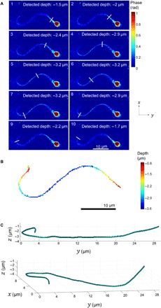
(A) Digital focusing in action. The white segment moves along the flagellum from the neck to the distal end, in the order indicated by the numbers in the top-left corners, finding the ultimate focus at each location. Color bar indicates phase values in radians. All the images shown are retrieved from a single digital off-axis hologram, acquired in a single camera shot. See dynamic representation in movie S1. (B) 2-D representation of the 3-D segmentation, where the color map indicates the recovered depth (z coordinate). (C) 3-D segmentation result from two viewpoints. See dynamic representation in movie S2.

In the analysis described above, we treated the entire flagellum as a single pixel-thin unit. However, the portion of the flagellum closest to the sperm head, the midpiece, is a thicker region composed of a central filamentous core encircled by many mitochondria. The cylindrical axisymmetrical morphology of the midpiece and the fact that it cannot be regarded as a single rigid body together with the sperm head do not allow for the same orientation recovery principles applied for the sperm head to be applied here. We therefore divided all flagellum pixels into two groups: midpiece region and non-midpiece region, and calculated a global average (over all frames) of the maximal phase value and width of the section for each group. These average values were then used to calculate the integral (thickness-averaged) RI for each region (24), under the assumption that each region is a cylinder, such that the thickness of the central pixel is equal to the width of the section. Further details are provided in the “Flagellum integral RI evaluation” section.

Last, the full dynamic reconstruction of the entire sperm cell can be attained by combining the 4-D segmentation results for the flagellum with the 3-D RI reconstruction of the head and 3-D orientation of the head retrieved for each frame. Figure 4 presents the full 4-D reconstruction results obtained from 1000 frames recorded during free swim in modified human tubal fluid (HTF) supplemented with 7% polyvinylpyrrolidone (PVP), which creates a viscous fluid commonly used in human ICSI to slow down sperm movement. Voxels, attributed to the midpiece or the rest of the flagellum, are represented by disk of constant diameter, which is equal to the calculated average width of the respective area. Figure 4A shows 4 frames (each in a different color) from the 3-D motion in movie S3, and Fig. 4B shows 15 frames from the same 3-D motion movie, where frames of earlier times are more transparent. Figure 4C shows a single frame from the 3-D motion revealing the internal structure of the sperm cell, for the same cell shown in Figs. 2 and 3. The integral RI was found to be 1.383 in the midpiece and 1.365 in the rest of the flagellum. Figure 4D shows the 3-D trajectory of the sperm cell head centroid, changing from blue to red as time progresses. The path shown in Fig. 4D falls under the category of the “typical” trajectory (9)—the most prevalent swimming pattern observed among human sperm cells (>90% of cells)—where the sperm head moves forward swiftly along a slightly curved axis with a small arbitrary lateral displacement (approximately 4 μm side to side) in either direction orthogonal to the flow.

Fig. 4. Full 4-D reconstruction of a sperm cell, obtained from 1000 frames recorded during free swim in 7% PVP.

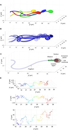
(A) Overlay of four frames from the 3-D motion in movie S3, each assigned with a different color. (B) Overlay of 15 frames from the 3-D motion in movie S3, each assigned with a different opacity, where earlier times are more transparent. (C) A single frame from the 3-D motion in movie S3, revealing the internal structure of the sperm cell. Light purple indicates the cell membrane (1.355 ≤ RI < 1.37), green indicates the midpiece (RI = 1.383), yellow indicates the acrosomal vesicle (1.37 ≤ RI < 1.425), red indicated the nucleus (1.425 ≤ RI < 1.465), and dark purple indicates RI ≥ 1.465 (centriole region). (D) Different views of the 3-D head centroid trajectory, changing from blue to red as time progresses.

To further validate the proposed technique, we also imaged sperm cells from another donor in HTF but, this time, without PVP, a challenging task due to faster movement of the sperm cells. We then compared the natural 3-D motion of the cell in free swim to this obtained after adding 5 mM caffeine, which is known to increase sperm motility without influencing its velocity (25). Movie S4 shows bright-field imaging of sperm cells in HTF with 7% PVP, without PVP, and without PVP but with 5 mM caffeine. The results of applying the suggested 4-D imaging method for comparing the motion of sperm cells of the same donor in HTF with and without caffeine can be seen in movie S5. The bottom video, showing the sperm cell treated with caffeine, presents more notable 3-D movement of the tail with flatter head movement.

We have imaged several more sperm cells swimming freely, resulting in similar 3-D RI distributions. Results for two additional sperm cell heads are given in fig. S5.

DISCUSSION

We presented a highly detailed, stain-free 4-D imaging method for capturing the entire sperm cell during free swim, including both the head with its internal organelle morphologies and the flagellum, based on a single-channel holographic video. We demonstrated the method both with and without the use of two motion-altering substances, PVP and caffeine, validating its ability to capture various types of 3-D movements. Other than the clear benefit for clinicians, allowing 4-D visualization for a more informed selection of sperm cells, this reconstruction enables calculation of the volume and dry mass for each of the organelles, thus adding previously inaccessible quantitative parameters for clinical use or biomedical assays.

The suggested method uses optical tomography, which is enabled by the fact that sperm cells rotate their head during swim, allowing access to their interferometric projections by the proposed algorithms. This is a unique case among human cells. Other types of cells with rapid dynamics, such as cardiomyocytes, cannot be straightforwardly imaged by the proposed method but rather need to rely on rapid illumination rotation with limited scanning angle range [e.g., (18)]. Thus, the suggested method assumes progressive sperm cells with typical repetitive rotation of the sperm head, including continuous unidirectional rolling across 360°, a condition that is fulfilled for most of the cells, as we have observed from the acquired data. In addition, it assumes that a single cell crosses the field of view each time. Sufficient acquisition framerate is crucial both for applying the temporal proximity principle in the 4-D segmentation of the flagellum and for properly recovering the 3-D orientation of the sperm head. For 4-D segmentation of the flagellum, as shown in the “Flagellum 4-D segmentation” section, the average displacement between consecutive frames should be 1 pixel or less. For recovering the orientation of the head, the affiliation of the roll angle to the different quadrants, as well as the sign determination of the pitch angle, relies on sufficient temporal sampling. For the former requirement, which is typically more demanding, the two extrema at 0° and 180° need to be detected for each full sperm head revolution. Thus, according to Nyquist’s theorem, the minimal required framerate is defined as four frames per full revolution (360° roll) of the sperm head. Nevertheless, accuracy improves markedly with much higher framerates. Specifically, the results obtained in this paper were taken at 2000 fps, and the sperm head rotated at 8 revolutions/s; thus, we had approximately 250 frames per full head revolution. Another demand for tomographic reconstruction is an overall sufficient number of projections to properly fill the 3-D Fourier space of the object; yet, this does not necessarily mandate a high framerate and thus is a weaker requirement. The results obtained in this paper used 1000 frames, taken over four full head revolutions.

The difficulty in tracing the flagellum, which is as thin as the resolution-limited spot and thus might be easily masked by coherent noise, can be reduced using a low-coherence light source, thus increasing the sensitivity of the 4-D localization task. For the task of 4-D localization of the flagellum, it is effectively treated as a superposition of point-like scatterers, which may reduce accuracy for “singular” orientations of the flagellum relative to the camera, such as rod-like segments aligned along the optical axis. Sperm cells swimming toward the camera may also cause difficulties in recovering the head orientation, as in these cases, the major radius may effectively turn into the minor radius of the projection and vice versa. Nevertheless, for sperm cells swimming in a perfusion chamber parallel to the camera, we have found that this scenario is rare.

In the analysis performed for the sperm head, we assume that the sperm cell head is a rigid body, which is a reasonable assumption due to a low confinement and flow rate (20), other than negligible deformation in the distal edge. We also assume that the internal structure of the sperm head remained constant throughout the recording process, and only its orientation changed. In the results presented in this manuscript, the head RI reconstruction was based on four head revolutions, recorded over half a second, thus enabling the RI distribution to be updated twice every second during free swim.

Considering the fast acquisition rates, efficient digital implementation of the suggested algorithms has the potential to allow near real-time visualization. The head recovery process has to be performed once per sperm cell, using the first few hundreds of frames, to obtain the model constants and the 3-D RI reconstruction of the head. Afterward, the orientation recovery for new frames can be updated in small groups in real time. Regarding 3-D tomographic reconstruction of the head, we have previously shown that using a conventional computer graphic processing unit (GPU), the processing time for a full 3-D tomographic reconstruction neglecting diffraction, based on 73 256 × 256 pixel projections with known orientations, can be reduced to 0.007 s (26). In the current paper, we used 1000 128 × 128 pixel projections to reconstruct the sperm head 3-D RI, indicating that similarly fast processing rates would be possible using a GPU for this case. In the current paper, however, we have used the more accurate version that takes diffraction into account in a central processing unit (CPU)–based implementation. Therefore, it took roughly 1 min to run a full reconstruction on an Intel i7-4790 CPU with 16 GB RAM. Full real-time implementations of the other parts of the algorithm, including flagellum 4-D segmentation, head focusing, and angle recovery, which are inherently more time consuming, are yet to be implemented.

To conclude, we presented a method enabling full 4-D reconstruction of freely swimming human sperm cells from an off-axis holographic video. This new method allows live sperm head internal structure and flagellum 3-D fine-detail dynamics to be imaged simultaneously during the sperm cell free swim, which is very challenging because of the fine-structures/fast-dynamics duality characterizing individual sperm cells. This approach allows calculation of unique quantitative parameters that could improve sperm choice, such as the dry mass and volume of the nucleus, which consists of the genetic materials, with the ability of correlating these parameters to the cell motion. We thus believe that this method will eventually allow selecting the best sperm cell for injecting into the ovum in ICSI. It is also expected that this method will be used to assess male fertility by 4-D computed tomography (CT) of the patient’s live sperm, providing an analysis of both the fine-detailed 3-D morphology and motility of the sperm on an individual-cell basis. In addition to assisting in vitro fertilization (IVF) procedures, the method presented here might aid in new biological studies. Specifically, we believe that the elevated RI values detected near the midpiece area are attributed to the centriole region. This organelle, which is crucial for the development of the embryo as it is introduced into the embryo only by the sperm, could not be imaged in live cells until now. Future biological studies may verify our hypothesis of increased RI in the centriole region using appropriate micromanipulation instrumentation and centriole-specific staining, as well as the correlation between the identification of this region and successful fertilization.

MATERIALS AND METHODS

Optical setup for interferometric phase microscopy

Figure S6 presents the optical setup used in this paper. Light from a helium-neon laser source illuminates the sample in an inverted microscope, composed of a 100× oil-immersion microscope objective (Olympus UPLSAPO 100 × O; numerical aperture, 1.4), and an achromatic tube lens of focal length 150 mm. The resulting sample beam then enters the off-axis external interferometric module (27, 28), where it is split into two beams of equal intensity by a 50:50 beam splitter. The first beam is focused onto a laterally shifted retroreflector mirror, RR1, by the first module achromatic lens, L1, of focal length 100 mm, causing a small shift in the illumination angle on the camera, producing off-axis interference. The second beam exiting the beam splitter is focused by lens L1 onto a 15-μm pinhole placed in the Fourier plane of the lens, thereby removing all the high spatial frequencies containing the sample information and thus creating a clean reference beam. The reference beam is then reflected back to the beam splitter by retroreflector mirror RR2. The two beams then merge in the beam splitter and, after passing through another achromatic lens L2 (focal length, 150 mm) and an additional magnifying 4f system composed of achromatic lenses L3 (focal length, 30 mm) and L4 (focal length, 75 mm), an off-axis image hologram is created on an ultrafast digital camera (FASTCAM Mini AX200, Photron; square pixels of 20 μm each, 1024 × 1024 pixels, 2000 fps). The entire optical system has a total magnification of ×328 and a resolution limit of 452 nm.

Biological preparation

A semen sample was collected in accordance with Tel Aviv University’s institutional ethical committee, from healthy 18- to 45-year-old donors, after undergoing 24 hours of abstention. After ejaculation, the sample was allowed to liquefy for 30 min. Following this, sperm cells were isolated from the semen fluid using a PureCeption bilayer kit (ORIGIO, Målov, Denmark) in accordance with the manufacturer’s instructions. In short, 0.5 ml of semen was placed on top of a 40 and 80% silicon bead gradient and centrifuged for 25 min at 1750 rpm. After centrifugation at 1250 rpm for 5 min, the supernatant was discarded, and the pellet containing the living sperm cells was washed with 10 ml of HTF (Irvine Scientific, CA, USA). After additional centrifugation, the supernatant was removed, and cells were resuspended in 2 ml of HTF supplemented with 7% PVP, 360,000 molecular weight (mw) (PVP360, Sigma-Aldrich). One milliliter of the cell solution was then placed in a chamber (CoverWell, PC1L-0.5; 32-mm width by 19-mm length by 0.6-mm depth, 1.5-mm diameter ports) for imaging. For the comparison in movie S5, PVP was not added, and after imaging the cells in their natural state, 5 mM caffeine was added.

Algorithm

Wavefront propagation

An interferometric system is able to record the entire wavefront that propagated through a sample, rather than just its intensity, by interfering it with a reference wavefront, yielding a digital hologram or interferogram (29). The resultant hologram is given by the following expression

$$\begin{array}{c}{\mid E_{\mathrm{s}}(x,y)+E_{\mathrm{r}}\mid }^2={\mid E_{\mathrm{s}}(x,y)\mid }^2+{\mid E_{\mathrm{r}}\mid }^2+\\ A_{\mathrm{s}}(x,y)A_{\mathrm{r}}\text{exp}[j{\mathrm{\phi }}_{\mathrm{s}}(x,y)-j{\mathrm{\phi }}_{\mathrm{r}}]+A_{\mathrm{s}}(x,y)A_{\mathrm{r}}\text{exp}[j{\mathrm{\phi }}_{\mathrm{r}}-j{\mathrm{\phi }}_{\mathrm{s}}(x,y)]\end{array}$$ (1)

where j denotes the imaginary unit, and E_s(x,y) = A_s(x,y)exp[jφ_s(x,y)] and E_r = A_rexp[jφ_r] are the sample and reference complex wavefronts, respectively (the latter assumed to be of constant phase and amplitude). Thus, the wavefront that propagated through the sample is fully conserved, although its extraction remains difficult. In off-axis holography, one of the interfering beams is titled at a small angle relative to the other, creating a linear phase shift that allows separation of the field intensity from the two complex-conjugate wavefront cross-correlation terms in the spatial frequency domain, thus allowing reconstruction of the complex sample wavefront from a single off-axis digital hologram. In this work, the complex wavefront was extracted from the raw hologram in the spatial frequency domain using a Fourier space–filtering algorithm (30), which cropped one of the cross-correlation terms, and then applied an inverse Fourier transform to obtain the complex wavefront. For efficiency reasons, the images were left at their cropped dimensions, four times smaller than the original hologram dimensions. Following this, the Rayleigh-Sommerfeld (RS) propagator was used to reconstruct the complex field at various distances from the recorded plane of focus (31), a propagation method suitable for weakly scattering objects (such as the sperm cell flagellum) (32). We took advantage of the transition to the Fourier space needed for isolating the wavefront and used the Fourier formulation of the Rayleigh-Sommerfeld propagator, simply requiring a pixel-wise multiplication of the cropped cross-correlation term with the following transfer function (31)

$$H_{\text{RS}}(u,v,z=d)=\{\begin{array}{c}\text{exp}\left[j\frac{2\mathrm{\pi }{n}_{\mathrm{m}}d}{\mathrm{\lambda }}\sqrt{1-{(\mathrm{\lambda }u)}^2-{(\mathrm{\lambda }v)}^2}\right],\text{for}\sqrt{u^2+v^2}<\frac{1}{\mathrm{\lambda }}\hfill \\ 0, \text{otherwise}\hfill \end{array}$$ (2)

where d is the distance to be propagated, n_m is the RI of the surrounding medium, j is the imaginary unit, and λ is the illumination wavelength. Thus, the wavefront propagation may be regarded as a linear, dispersive, spatial filter with a finite bandwidth. The refocused wavefront at z = d can then be obtained by applying an inverse 2-D Fourier transform on the result. The spacing between the different reconstruction planes was chosen to be exactly the effective pixel size of the image (which was identical for horizontal and vertical coordinates), resulting in a pseudo-volume with isotropic sampling frequency. The boundaries of the propagation distance can be determined by the maximal depth allowed by the physical restriction used in the experiment. To prevent excessive memory use, a propagation distance of 16 μm is used in this paper, taking into consideration that the human flagellum is approximately 60 μm long, assuming that the sperm is not swimming toward the camera.

Handling high noise levels

One of the greatest challenges of tracing the 3-D location of the flagellum per each frame is finding the pixels associated with the tail in the 2-D image, i.e., performing 2-D segmentation. This is a complex task due to the low-phase values of the flagellum, which are similar to the noise level when using a coherent light source, especially for out-of-focus segments. We thus constructed a targeted, adaptable, locally conserving cleaning (TALCC) function, which identifies the important parts of the image that need to be locally conserved. What makes this function highly targeted and adaptable is its multiple inputs, including not only the original phase image but also the current binary segmentation map, row and column of interest, slope in region of interest, and noise level mode. The noise level mode, adapted automatically in our analysis, starts at a value of 0, indicating a neutral input, and can take higher positive values for dealing with increasingly higher noise levels that require robust cleaning or lower negative values for dealing with thin, low-contrast segments that need delicate cleaning. The row and column of interest, together with the slope in region of interest, are used to define a 3 × 6 pixel environment around the row and column of interest that needs to be preserved, defined as 1 pixel to each side, 4 pixels forward and 1 pixel backward, rotated in the direction of the slope. The input phase map is first thresholded to obtain a binary image, with a threshold value respective to the noise level mode; then, both the pixel group defined by the 3 × 6 pixel environment and the pixel group marked as the object in the current (and previous frame, if available) segmentation map are marked as the object in the binary image. At this point, morphological opening and closing (33) are subsequently applied to clean noise and close holes, respectively, with parameters according to the automatically detected noise level mode. The structuring elements used are lines with a slope either parallel or orthogonal to that of the region of interest, thus preserving segments with similar direction and erasing others. In the case of low-contrast segments, indicated by a negative noise level mode, the closing operation is applied before the cleaning operation, and the structuring elements used are disk shaped.

Seed points

To aid the segmentation process in the low signal-to-noise-ratio conditions, we find a good (x,y,z) starting point in each frame, namely, a “seed point,” which is ideally the neck area connecting the sperm head and midpiece. Toward this end, all frames are first rotated according to the optical flow (34), such that the overall swimming direction of the cell is left to right. We start from the first frame, guessing the z coordinate of the seed point to be at the middle of the range (i.e., the z = 0 plane). We then reconstruct the modulus of the phase profile at this initial depth, where the modulus operation is needed because of phase-unwrapping problems that may occur in out-of-focus regions, and use it to calculate a binary mask of the head and midpiece areas. This is done by taking a low threshold (~0.25 radians), zeroing out most of the flagellum area, but not the slightly elevated phase values of the midpiece area, and then applying morphological opening and closing. The orientation of the ellipse that has the same normalized second central moments as the binary mask is then calculated, indicating the estimated slope at the neck (S_n). The depth range for the search is determined by a fixed window parameter, which should be larger for the first frame, as the initial depth estimation is a guess, such that continuity is not expected. For each depth in the search area, a new binary mask of the sperm head and neck is calculated with a slightly higher threshold (~0.4 radians) as to exclude most of the flagellum, but not the midpiece. Then, the orientation of the ellipse that has the same normalized second central moments as the binary mask is calculated and used to rotate the head to a horizontal position. In this horizontal position, morphological opening with a vertical line–structuring element is applied, effectively erasing the midpiece area with minimal damage to the rest of the cell, such that the leftmost column indicates the seed point. The length of the midpiece (used in the “Flagellum integral RI evaluation” section) can then be evaluated by taking the difference between the original and cleaned rotated binary maps and calculating the major axis length of the remaining object. After flagging this point, the mask can be rotated back to its original position, thereby determining the actual row and column of the seed point. Following this, a line centered in the x-y location of the seed point and orthogonal to the neck, the direction of which was determined by S_n, is retrieved from the phase image cleaned by the TALCC function. This line is used to determine the ultimate focus location of the x-y seed point by recovering numerous parameters. First, the line is fitted with a Gaussian, from which the width, expected value, amplitude, and maximal value of the section are determined. Second, the number of maxima points in the original line values is determined. Last, the sum of the absolute gradient of the line values in the amplitude image is calculated (35). Then, the smoothed width vector, amplitude vector, and sum of the absolute gradient vector, obtained for the entire depth range, are used to calculate a triple score vector, given by the element-wise multiplication of the sum of the absolute gradient and width vectors divided by the amplitude vector. The depth with the lowest score—thus with the steepest, most narrow Gaussian and with the most transparent amplitude image—corresponds to the ideal focus plane, yielding the depth of the seed point (z_s). To prevent poorly fitted Gaussians from corrupting the results, unreasonable parameters such as multiple maxima points, a negative amplitude, or an extremely high or low expected value all cause the respective score to be replaced with a high constant score, used as a flag. Third, the expected value retrieved from the Gaussian of the chosen depth is used to update the exact (x_s,y_s) location of the seed point.

We repeat this process for all frames, where each time the initial z coordinate of the seed point is the one found from the previous frame [z_s(t − 1)], working under the assumption that the data are smooth enough because of the high framerate. Last, we further use the expected smoothness between frames by applying a smoothing filter for each seed coordinate vector: x_s, y_s, and z_s.

Flagellum 4-D segmentation

To apply 3-D segmentation of the sperm cell flagellum, for each frame we iterate within a loop that begins with the seed point of that frame [x_s(t), y_s(t), z_s(t)] and runs until it reaches either the boundaries of the image or a stopping criterion. This means that this algorithm can only trace parts of the tail that are connected to each other and not parts that exit the field of view and return in a secondary location. Within this loop, we run a recursive function (see the detailed algorithm given in the Supplementary Materials), which outputs the coordinates of the next voxel associated with the tail as well as a flag parameter, indicating whether we have reached the stopping criterion. This function takes, as an input, the coordinates of the last voxel that has been identified, the reconstructed complex field stack for that frame, two types of location maps, an iteration-counting parameter, the slope of the current segment, the noise level mode, and a validity flag variable initialized as a positive integer. The first type of location map stores nonzero values in (x,y) locations identified as being associated with the flagellum, and the second type is based on the first type of the previous frame. Figure S7 shows two such location maps, where the map shown in A is the original binary location map restored from frame t and the map shown in B is a weighted, dilated version of it, used for preventing deviation from the flagellum in frame t + 1. For the first iteration of each frame, we use the coordinates of the seed point, the estimated slope at the neck (S_n) calculated in the “Seed points” section, and a neutral, zero noise level mode. For the first frame processed, we use an altered version of the function that does not require the use of the second type of location maps.

The recursive function is composed of four main parts. In the first part, we evaluate the direction of the current segment, which is centered on the previous pixel (x_o,y_o) in the initial phase image. This initial phase image is reconstructed at depth z_o (estimated for the previous pixel) and cleaned by pixel-wise multiplication with the weighted, dilated version of the location map of the previous frame. Next, this direction is used to define a directional environment to search the initial phase image for the coordinates of the next voxel associated with the tail, (x_i,y_i). In the second part, the z_i location of (x_i,y_i) is recovered. This is achieved by first finding the possible range of depths based on continuity and smoothness considerations, both relative to the current and previous frames, and then examining a linear section of the respective depth phase image centered around (x_i,y_i), orthogonal to the direction of the current segment, for the calculated depth range. In this process, we calculate a score expressing the likelihood of every depth in this range to be the location of optimal focus, based on the distance from the center of the estimated depth range, the width, and the maximal phase value of the section. The validity of the score is then verified by a second set of parameters, including the estimated maximal phase value, width, standard deviation, and phase profile shape, to estimate whether the score is valid, more/less robust cleaning is required, or the end of the flagellum was reached. In the third part of the function, the validity score is evaluated and used to decide whether to call the function again with a higher/lower noise level mode, finish the function normally, or finish the function with a flag indicating that the end of the tail may have been detected. Last, in the fourth part of the function, executed only once for the recursion base with the updated noise level mode value, we repeat the first part using the updated depth z_N, estimated at the second part. If the phase value of (x_N, y_N, z_N) is below a fixed threshold, we finish the function with a flag indicating that the end of the tail may have been detected.

For each frame, we iterate until we reach a stopping criterion based on cumulative indications that the end of the flagellum may have been detected. If the flagellum detection has ended before exiting the field of view, then we check the Euclidean distance between the current and previous end point; if it is larger than a fixed threshold, we assume that an error has occurred in this specific frame (as may occur because of high local noise), define this frame as invalid, and use the previous frame again instead, slightly increasing the distance tolerance for the next frame.

Flagellum integral RI evaluation

To calculate the integral RI value of the flagellum, we first classify all flagellum pixels into two groups: midpiece and non-midpiece. For this purpose, we evaluate the length of the midpiece at the detected seed point depth (see the “Seed points” section) in each frame. Based on the 4-D segmentation of the flagellum, we found that the average pitch angle of the midpiece is approximately 9°. Since the actual midpiece length is the length measured in the quantitative phase projection divided by the cosine of the pitch angle, the average error induced by not considering the pitch is only 1% of the midpiece length. Therefore, we have chosen to use the average midpiece length over all frames to classify the pixels identified as flagellum pixels according to Euclidian distance from the seed point. Note that a few dozen frames are enough to determine the length of the midpiece. To prevent bent tail positions from causing false association to the midpiece, once the first non-midpiece pixel is detected, all future pixels of that frame are declared non-midpiece as well. Next, the average of each group for the section width and maximal phase value parameters of the chosen depth, estimated in the second part of the recursive function described in the “Flagellum 4-D segmentation” section, is calculated over all frames. Assuming that the midpiece and non-midpiece portions of the flagellum can each be modeled as a cylinder, the thickness of the central pixel is equal to the width of the section; thus, the integral RI of each group can be calculated as follows

$$n=n_{\mathrm{m}}+\frac{\mathrm{\lambda }{\mathrm{\phi }}_{\text{max}}}{2\mathrm{\pi }\mathrm{\omega }\mathrm{\Delta }x}$$ (3)

where n_m is the RI of the surrounding medium; λ is the wavelength; ∆x is the length of each pixel, calculated as the ratio between the sensor pixel size and the total magnification; φ_max is the average maximal phase value of the section for the group; and w is the average section width in pixels for the group.

Head focusing

To retrieve the focus of the sperm head, we start from the first frame, guessing the optimal focus location of the head to be at the middle of the range (i.e., the z = 0 plane). We then reconstruct the modulus of the phase profile at this depth and use it to calculate a binary mask of the head area. This is done by taking a low threshold (~0.25 radians), followed by morphological opening and closing. Then, the binary mask undergoes dilation to include the area that will be occupied by the head in out-of-focus frames. The depth range for the search of optimal focus is determined by a fixed window parameter, which should be larger in value for the first frame, as the initial depth estimation is a guess, such that continuity is not expected. For each depth in the search area, we calculate the sum of the absolute gradient of the amplitude image in the region defined by the binary mask (which should be minimal at the plane of focus for pure phase objects such as biological cells), the sum of the negative values of the phase image in the region defined by the binary mask (which is indicative of phase-unwrapping issues characteristic of out-of-focus frames), and the Tamura coefficient [a sparsity metric; (36)] of the gradient of the complex field in the region defined by the binary mask.

Following this, the smoothed parameter vectors obtained for the entire depth range are used to calculate a triple score vector, given by the element-wise multiplication of the first two divided by the third. The depth with the lowest score corresponds to the ideal focus plane.

Head segmentation

To achieve more precise segmentation, all quantitative phase images were resized to be four times larger, returning them to the original hologram dimensions. For each frame, the segmentation of the sperm cell head from the original image consists of rough segmentation and fine segmentation. Initially, in the rough segmentation, the original image is segmented using a threshold of 0.6 radians on the phase values, followed by morphological closing and opening. This initial segmentation is used to estimate the centroid of the remaining object (which is mostly the head and possibly some of the midpiece), allowing the image to be cropped such that it is centered on the head. Following this, the orientation of the ellipse that has the same normalized second central moments as the binary mask is calculated, allowing the image to be rotated such that the head is placed horizontally, with the neck at the left and the acrosome at the right. Next, fine-tuning of the segmentation is performed. At this step, we exploit the fact that the acrosome is in the right half of the image to apply more intensive, targeted cleaning to the left part, effectively and accurately erasing the midpiece area from the unsegmented phase image, leaving only the head. This is important since, for frames where the sperm cell is rotated on its side, the acrosome area becomes very thin at the midpiece area and may be accidently erased if this cleaning is applied to the entire image. Thus, for the left third of the image, we apply a threshold of 0.9 radians on the phase values, followed by morphological opening with a structuring element that is a vertical line (unlike the usual disk-shaped structuring element), effectively erasing the midpiece area with minimal damage to the rest of the cell. For the right two-thirds of the image, we only apply a much lower phase threshold of 0.35 radians. The resultant binary mask is then used to more accurately center and rotate the image, as well as to extract the minor and major axis radii of the ellipse that has the same normalized second central moments. Centering is performed for the bounding box enclosing the binary mask.

Head orientation recovery

To estimate the 3-D orientation of the sperm cell head for each frame, we model it to be an ellipsoid, according to

$${(x/A)}^2+{(y/B)}^2+{(z/C)}^2=1$$ (4)

where it can be assumed from the standard dimensions of sperm cell heads that B ≫ A > C (see Fig. 1). This process finds the final orientation of the sperm head that yields the same projected ellipse as the rotated ellipsoid model and not necessarily the stand-alone values of the pitch, roll, and yaw angles as 3-D rotation is not commutative (i.e., the order of rotation matters). The determination of the model constants (A,B,C), as well as the affiliation of the pitch, roll, and yaw angles to the different frames, relies completely on the minor and major axis radius vectors calculated for the binary masks of the respective projections of the head (as explained in the “Head segmentation” section). Thus, to prevent possible localized segmentation errors from corrupting the results, we apply a smoothing filter to each vector, relying on the smoothness that can be expected at high framerates. Examples of the major and minor radius vectors obtained for a sperm cell, before and after smoothing, are shown in fig. S8, demonstrating the repetitive nature of sperm head rotation during free swim.

Finding the roll angle for each frame

We define the roll angle θ to be the rotation around the longitudinal axis of the sperm cell head (y axis in Fig. 1). Because of the periodic nature of sperm head rolling during free swim, as demonstrated in fig. S8A, constants A and C can be reliably estimated as the maximal and minimal values of the minor radius vector, respectively. Once constants A and C are known, and under the ellipsoid model assumption, the roll angle associated with each frame can be inferred within a 90° range from the minor radius of the projection. Practically, this can be done by calculating half the length of the projection of the ellipse shown in Fig. 1 for a finite number of rotation angles in a 90° range and then using interpolation to pinpoint the exact angle θ₉₀ suitable for every measured minor radius length. To retrieve the angles over a 360° range, continuity considerations can be made to find the proper quadrant, as long as a high framerate is maintained. For example, we can label each segment between two extrema with a sequential integer N_q and retrieve the angle within a 360° range by applying the following rule

$${\mathrm{\theta }}_{360}=\{\begin{array}{ccc}{\mathrm{\theta }}_{90},\hfill & \text{if}\hfill & N_q\text{mod} 4=1\hfill \\ 180-{\mathrm{\theta }}_{90},\hfill & \text{if}\hfill & N_q\text{mod} 4=2\hfill \\ 180+{\mathrm{\theta }}_{90},\hfill & \text{if}\hfill & N_q\text{mod} 4=3\hfill \\ 360-{\mathrm{\theta }}_{90},\hfill & \text{if}\hfill & N_q\text{mod} 4=0\hfill \end{array}$$ (5)

Note that relying on locating extrema defines the minimal required framerate to be four frames for a full revolution, yet accuracy improves markedly with much higher framerates. For example, fig. S8A shows approximately 250 frames per full revolution.

Last, the direction of the rolling has to be addressed. The sperm cell can rotate either clockwise or counterclockwise and can generally change its rotation direction during swim. Nevertheless, for the short recording duration needed for the reconstruction, we assume that the rotation direction is constant, a valid assumption for a smooth, periodic minor axis vector as the one shown in fig. S8A. To automatically determine the directionality of the rotation for each sperm cell, we observe the 3-D vector indicating the location of the neck over time (the seed point found in the “Seed points” section). Specifically, assuming that the forward motion of the sperm is primarily in the y direction, we are interested in the x and z coordinate vectors. To determine rolling polarity, we calculate the gradient (numerical difference) of the x coordinate vector, g_x, and use it to calculate two parameters: V_H, which is the sum of all z coordinate values of frames for which g_x > 0, and V_L, which is the sum of all z coordinate values of frames for which g_x < 0. Then, if V_H > V_L, we determine the rotation direction to be clockwise and vice versa. The logic behind this method is depicted in fig. S9. If for a positive change in x (blue arrows) we obtain higher values of z than for a negative change in x, then we are in the case depicted in fig. S9A; otherwise, we are in the case depicted in fig. S9B. Note that this calculation can be applied in an identical manner by switching the roles of x and z (and calculating g_z). If the rotation is counterclockwise, we simply need to correct the roll angles to be θ = −θ₃₆₀. Note that this calculation has to be performed only once for the first few dozen of frames, assuming that the cell does not change its rotation polarity.

Finding the pitch angle for each frame

We define the pitch angle χ to be the elevation of the head relative to the camera (x-y) plane (i.e., rotation around the x axis in Fig. 1). The pitch angle is related to the major axis radius, yielding a maximal value whenever the sperm cell head is aligned with the camera plane (i.e., χ = 0). Thus, zero crossings of χ, which are sign-switching events, can be found from the global positive extrema of the major radius vector. Generally, for freely swimming sperm cells, the pitch angle displays a more complex rotation pattern than the roll angle. For example, the pattern exhibited in fig. S8 shows a zero crossing for χ after every full revolution in θ. The correlation between the peaks in the major and minor radius vectors, where the global positive extrema of the major radius vector are a subset of the negative extrema of the minor radius vector, allows us to determine the zero crossings of χ in a more reliable manner that is less sensitive to noise. The missing constant of the model (B) can then be found from the average value of the global positive extrema in the major radius vector. Once all three constants are found, the pitch angle associated with each frame can be inferred from the major radius of the projection. Practically, this is done by rotating the 3-D ellipsoid according to the recovered roll angle θ for that frame and then rotating it for a finite number of pitch angles within a 50° range, followed by calculating the major axis radius of each resultant projection. Then, interpolation is used to pinpoint the exact pitch angle value χ suitable for every measured major radius length. Note that a larger range than 50° is redundant as long as the primary forward motion of the sperm cell is in the y direction. If this is not the case, then this method may be unsuitable, as the major radius may effectively turn into the minor radius of the projection for higher pitch angles.

Once the value of the pitch angle is found for all frames, we assign it with a proper sign, where each zero crossing of χ is expected to cause a sign switch, and we need to choose whether the even or odd segment numbers receive a negative sign. To determine this, we compare the z location vector of the neck, z_neck (found in the “Seed points” section), to the z location vector of the head, z_head, as found in the “Head focusing” section. Naively, we may expect z_head > z_neck for χ > 0 and vice versa. Practically, however, this condition is not always fulfilled for every sample. Nevertheless, if we check the overall trend per segment between two zero crossings of χ, it allows us to reliably estimate which segments are positive and which are negative.

Finding the yaw angle for each frame

We define the yaw angle a to be the rotation in the camera (x-y) plane (i.e., rotation around the z axis in Fig. 1). The recorded yaw angle a has already been found from the orientation of the ellipse that has the same normalized second central moments as the binary mask in the “Head segmentation” section and should not be an input to tomographic reconstruction, as we have already rotated all sperm cell heads in −a to achieve a horizontal position. However, for nonspherical objects, the combination of nonzero roll and pitch inevitably creates a small yaw angle a₀, which should be calculated and compensated when preparing the phase image to be located in the native position for the tomographic reconstruction. This small angle can be found for each frame by rotating the 3-D ellipsoid model according to the previously calculated roll and pitch angles and then calculating the orientation of the ellipse that has the same normalized second central moments as the binary mask of the resultant projection. Note that for recovering the 3-D orientation of the sperm cell head for movement reconstruction, we impose a yaw angle of a − a₀, mimicking the measured yaw angle.

Tomographic reconstruction

ODT is a well-established technique, which enables reconstruction of the 3-D RI distribution of an object from a set of digital holograms taken from multiple viewing angles of the object. The diffraction algorithm can be implemented using either the Born or Rytov approximations (22), both of which take the incident field as the driving field at each point of the scatterer, and consider the scattered electrical field due to the presence of a sample. The Born approximation is valid only when the scattered field is smaller than the incident field and specifically when the overall phase difference induced by the object is substantially smaller than 2π (22, 37). As the phase values of sperm cells often approach ~5 radians in a watery medium when tilted on their side, this condition is not met for all phase images. The Rytov approximation for the diffraction algorithm, on the other hand, is valid as long as the phase gradient in the sample is small (22, 37–39), as is generally the case for biological cells, and is thus a reasonable choice for applying tomography on sperm cells (18).

When applying the Rytov approximation for the ODT algorithm, the Rytov field for each properly yaw-compensated and centered hologram, taken from viewpoint (θ,χ), is calculated as follows

$$u_{\text{Rytov}}(x,y\mid \mathrm{\theta },\mathrm{\chi })=\text{log}[\mid E_{\mathrm{s}}(x,y\mid \mathrm{\theta },\mathrm{\chi })\mid /\mid E_0(x,y)\mid ]+j\mathrm{\phi }(x,y\mid \mathrm{\theta },\mathrm{\chi })$$ (6)

where |E_s(x,y|θ,χ)| is the amplitude extracted from the sample hologram taken from viewpoint (θ,χ); |E₀(x,y)| is the amplitude extracted from a sample-free acquisition taken as a reference; φ(x,y|θ,χ) is the difference between the phase profile extracted from the sample hologram taken from viewpoint (θ,χ) and the phase profile extracted from a sample-free acquisition; and j is the imaginary unit. Each Rytov field profile taken from viewpoint (θ,χ) is then processed and mapped into a 2-D hemispheric surface (Ewald sphere) rotated in the same direction in the 3-D spatial Fourier space (22). This hemispheric surface is defined by the scattered wave vectors, which are given as follows for an incident untilted plane wave

$$k_{s,x}=p\mathrm{\Delta }k; k_{s,y}=q\mathrm{\Delta }k; k_{s,z}=\sqrt{{\left(\frac{{2\mathrm{\pi }n}_{\mathrm{m}}}{\mathrm{\lambda }}\right)}^2-k_{{s,x}^2}-k_{{s,y}^2}}$$ (7)

where p and q are the column and row indices defining the grid, respectively, n_m is the RI of the surrounding medium, λ is the illumination wavelength, and Δk = 2π / L is the spectral pixel size, with L being the length of the field of view. Then, pixels for which k_s,z ≤0 are discarded, as they fit evanescent waves. The initial locations on the 3-D grid, forming an Ewald sphere, are given by

$$k_x=p; k_y=q; k_z=\frac{1}{\mathrm{\Delta }k}(k_{s,z}-\frac{{2\mathrm{\pi }n}_{\mathrm{m}}}{\mathrm{\lambda }})$$ (8)

The 2-D profile to be mapped on the Ewald sphere rotated to position (θ,χ) is then calculated from the Rytov field profile taken at the same angle, according to

$$U(k_x,k_y\mid \mathrm{\theta },\mathrm{\chi })=2j{k}_{s,z}\odot {FT}_{2\mathrm{D}}\{u_{\text{Rytov}}(x,y\mid \mathrm{\theta },\mathrm{\chi })\}$$ (9)

where FT_2D denotes the 2-D discrete Fourier transform, and ⊙ is the Hadamard (element-wise) product. Here, too, pixels for which k_s,z ≤ 0 are discarded.

The three matrices k_x, k_y, and k_z from Eq. 8 are then reshaped to be vectors and stacked in three consecutive rows, forming the matrix A_L. For each hologram recorded from viewpoint (θ,χ), the 3-D location matrix M_L(θ,χ), is then given by

$$M_L(\mathrm{\theta },\mathrm{\chi })=\left[\begin{array}{ccc}\text{cos}(\mathrm{\theta })& 0& -\text{sin}(\mathrm{\theta })\\ 0& 1& 0\\ \text{sin}(\mathrm{\theta })& 0& \text{cos}(\mathrm{\theta })\end{array}\right]\cdot \left[\begin{array}{ccc}1& 0& 0\\ 0& \text{cos}(\mathrm{\chi })& -\text{sin}(\mathrm{\chi })\\ 0& \text{sin}(\mathrm{\chi })& \text{cos}(\mathrm{\chi })\end{array}\right]\cdot A_L$$ (10)

where the position in the nth dimension is given by the nth row of the resultant matrix M_L(θ,χ).

In the case discussed here, where there is no constant rotation axis that can be defined as one of the Cartesian axes, the available sampling points in the 3-D frequency domain are naturally unevenly distributed in the 3-D Cartesian grid, causing substantial artifacts. This can be partially resolved by an additional interpolating step for estimating the unknown spectral values on a predefined 3-D Cartesian grid (40). For this purpose, we used the inverse distance weighting interpolation method (41), which is based on the assumption that the frequency sample that is to be interpolated should be more strongly influenced by closely located neighboring samples than by remotely located neighboring samples, such that the value at the desired location is a weighted linear average of the neighboring values, where the associated weight decreases with distance. This can be mathematically formulated as follows

$$F_{\text{cartesian}}={\displaystyle {\sum }_{i=1}^N}{w}_i\cdot f_i, w_i=\frac{{h_i}^{-P}}{{\displaystyle {\sum }_{k=1}^N}{h_k}^{-P}}$$ (11)

where f_i represents the spectral value of the ith scattered frequency sample and w_i is its associated weight, calculated based on the relative inverse distance h between the weighted sample and the interpolation site. N and P are two important parameters of this method, where N is the number of neighbors considered and P is the weighting factor, where greater values of P assign greater influence to the values closest to the interpolated point. We chose N ≥ 30, implemented by looking for neighbors in a growing 3-D cube until at least 30 neighbors are encountered, and P = 4, according to a rule of thumb stating that for a D-dimensional problem, P ≤ D causes the interpolated values to be dominated by points far from the interpolation site.

Once all values on the 3-D grid are determined by interpolation, yielding the 3-D volume V, the 3-D RI distribution of the original object can be obtained by performing an inverse 3-D Fourier transform and applying the following formula

$$n(x,y,z)=\sqrt{{n_m}^2-\frac{{\mathrm{\lambda }}^2}{4{\mathrm{\pi }}^2}\cdot f(x,y,z)}$$ (12)

where n_m is the RI of the medium, λ is the illumination wavelength, and f(x,y,z) is the result of the inverse 3-D Fourier transform applied on the 3-D volume V. Note that the quality of tomographic reconstruction improves with the available number of viewpoints, where we used 1000 projections.

SUPPLEMENTARY MATERIALS

Supplementary material for this article is available at http://advances.sciencemag.org/cgi/content/full/6/15/eaay7619/DC1

REFERENCES AND NOTES

- 1.World Health Organization, Examination and Processing of Human Semen (World Health Organization, ed. 5, 2010).
- 2.Bartoov B., Berkovitz A., Eltes F., Kogosovsky A., Menezo Y., Barak Y., Real-time fine morphology of motile human sperm cells is associated with IVF-ICSI outcome. J. Andrology 23, 1–8 (2002). [DOI] [PubMed] [Google Scholar]
- 3.Bartoov B., Berkovitz A., Eltes F., Kogosovsky A., Yagoda A., Lederman H., Barak Y., Pregnancy rates are higher with intracytoplasmic morphologically selected sperm injection than with conventional intracytoplasmic injection. Fertil. Steril. 80, 1413–1419 (2003). [DOI] [PubMed] [Google Scholar]
- 4.Memmolo P., Di Caprio G., Distante C., Paturzo M., Puglisi R., Balduzzi D., Galli A., Coppola G., Ferraro P., Identification of bovine sperm head for morphometry analysis in quantitative phase-contrast holographic microscopy. Opt. Express 19, 23215–23226 (2011). [DOI] [PubMed] [Google Scholar]
- 5.Haifler M., Girshovitz P., Band G., Dardikman G., Madjar I., Shaked N. T., Interferometric phase microscopy for label-free morphological evaluation of sperm cells. Fertil. Steril. 104, 43–47.e2 (2015). [DOI] [PubMed] [Google Scholar]
- 6.Mirsky S. K., Barnea I., Levi M., Greenspan H., Shaked N. T., Automated analysis of individual sperm cells using stain-free interferometric phase microscopy and machine learning. Cytom. A 91, 893–900 (2017). [DOI] [PubMed] [Google Scholar]
- 7.Lim C. C., Lewis S. E., Kennedy M., Donnelly E. T., Thompson W., Human sperm morphology and in vitro fertilization: Sperm tail defects are prognostic for fertilization failure. Andrologia 30, 43–47 (1998). [DOI] [PubMed] [Google Scholar]
- 8.Corkidi G., Taboada B., Wood C. D., Guerrero A., Darszon A., Tracking sperm in three-dimensions. Biochem. Biophys. Res. Commun. 373, 125–129 (2008). [DOI] [PubMed] [Google Scholar]
- 9.Su T. W., Xue L., Ozcan A., High-throughput lensfree 3D tracking of human sperms reveals rare statistics of helical trajectories. Proc. Natl. Acad. Sci. U.S.A. 109, 16018–16022 (2012). [DOI] [PMC free article] [PubMed] [Google Scholar]
- 10.P. Memmolo, L. Miccio, F. Merola, P. A. Netti, G. Coppola, P. Ferraro, Investigation on 3D morphological changes of in vitro cells through digital holographic microscopy, in Optical Methods for Inspection, Characterization, and Imaging of Biomaterials, P. Ferraro, M. Ritsch-Marte, S. Grilli, D. Stifter, Eds. (SPIE, 2013), pp. 87920R. [Google Scholar]
- 11.Di Caprio G., El Mallahi A., Ferraro P., Dale R., Coppola G., Dale B., Coppola G., Dubois F., 4D tracking of clinical seminal samples for quantitative characterization of motility parameters. Biomed. Opt. Express 5, 690–700 (2014). [DOI] [PMC free article] [PubMed] [Google Scholar]
- 12.Jikeli J. F., Alvarez L., Friedrich B. M., Wilson L. G., Pascal R., Colin R., Pichlo M., Rennhack A., Brenker C., Kaupp U. B., Sperm navigation along helical paths in 3D chemoattractant landscapes. Nat. Commun. 6, 7985 (2015). [DOI] [PMC free article] [PubMed] [Google Scholar]
- 13.Silva-Villalobos F., Pimentel J. A., Darszon A., Corkidi G., Imaging of the 3D dynamics of flagellar beating in human sperm. Conf. Proc. IEEE Eng. Med. Biol. Soc. 2014, 190–193 (2014). [DOI] [PubMed] [Google Scholar]
- 14.Bukatin A., Kukhtevich I., Stoop N., Dunkel J., Kantsler V., Bimodal rheotactic behavior reflects flagellar beat asymmetry in human sperm cells. Proc. Natl. Acad. Sci. U.S.A. 112, 15904–15909 (2015). [DOI] [PMC free article] [PubMed] [Google Scholar]
- 15.Daloglu M. U., Luo W., Shabbir F., Lin F., Kim K., Lee I., Jiang J.-Q., Cai W.-J., Ramesh V., Yu M.-Y., Ozcan A., Label-free 3D computational imaging of spermatozoon locomotion, head spin and flagellum beating over a large volume. Light Sci. Appl. 7, 17121 (2018). [DOI] [PMC free article] [PubMed] [Google Scholar]
- 16.Mikami H., Harmon J., Kobayashi H., Hamad S., Wang Y., Iwata O., Suzuki K., Ito T., Aisaka Y., Kutsuna N., Nagasawa K., Watarai H., Ozeki Y., Goda K., Ultrafast confocal fluorescence microscopy beyond the fluorescence lifetime limit. Optica 5, 117–126 (2018). [Google Scholar]
- 17.Merola F., Miccio L., Memmolo P., Di Caprio G., Galli A., Puglisi R., Balduzzi D., Coppola G., Netti P., Ferraro P., Digital holography as a method for 3D imaging and estimating the biovolume of motile cells. Lab Chip 13, 4512–4516 (2013). [DOI] [PubMed] [Google Scholar]
- 18.Jiang H., Kwon J.-W., Lee S., Jo Y.-J., Namgoong S., Yao X.-R., Yuan B., Zhang J.-B., Park Y.-K., Kim N.-H., Reconstruction of bovine spermatozoa substances distribution and diff between Holstein and Korean native cattle using three-dimensional refractive index tomography. Sci. Rep. 9, 8774 (2019). [DOI] [PMC free article] [PubMed] [Google Scholar]
- 19.Charrière F., Pavillon N., Colomb T., Depeursinge C., Heger T. J., Mitchell E. A., Marquet P., Rappaz B., Living specimen tomography by digital holographic microscopy: Morphometry of testate amoeba. Opt. Express 14, 7005–7013 (2006). [DOI] [PubMed] [Google Scholar]
- 20.Merola F., Memmolo P., Miccio L., Savoia R., Mugnano M., Fontana A., D'Ippolito G., Sardo A., Iolascon A., Gambale A., Ferraro P., Tomographic flow cytometry by digital holography. Light Sci. Appl. 6, e16241 (2017). [DOI] [PMC free article] [PubMed] [Google Scholar]
- 21.Villone M. M., Memmolo P., Merola F., Mugnano M., Miccio L., Maffettone P. L., Ferraro P., Full-angle tomographic phase microscopy of flowing quasi-spherical cells. Lab Chip 18, 126–131 (2018). [DOI] [PubMed] [Google Scholar]
- 22.A. C. Kak, M. Slaney, Principles of Computerized Tomographic Imaging (SIAM, 2001). [Google Scholar]
- 23.De Angelis A., Managò S., Ferrara M. A., Napolitano M., Coppola G., De Luca A. C., Combined Raman spectroscopy and digital holographic microscopy for sperm cell quality analysis. J. Spectrosc. 2017, 1–14 (2017). [Google Scholar]
- 24.Liu L., Kandel M. E., Rubessa M., Schreiber S., Wheeler M. B., Popescu G., Topography and refractometry of sperm cells using spatial light interference microscopy. J. Biomed. Opt. 23, 025003 (2018). [DOI] [PubMed] [Google Scholar]
- 25.Moussa M. M., Caffeine and sperm motility. Fertil. Steril. 39, 845–848 (1983). [PubMed] [Google Scholar]
- 26.Dardikman G., Habaza M., Waller L., Shaked N. T., Video-rate processing in tomographic phase microscopy of biological cells using CUDA. Opt. Express 24, 11839–11854 (2016). [DOI] [PubMed] [Google Scholar]
- 27.Shaked N. T., Quantitative phase microscopy of biological samples using a portable interferometer. Opt. Lett. 37, 2016–2019 (2012). [DOI] [PubMed] [Google Scholar]
- 28.Girshovitz P., Shaked N. T., Compact and portable low-coherence interferometer with off-axis geometry for quantitative phase microscopy and nanoscopy. Opt. Express 21, 5701–5714 (2013). [DOI] [PubMed] [Google Scholar]
- 29.C. M. Vest, Holographic Interferometry (Wiley, 1979). [Google Scholar]
- 30.Girshovitz P., Shaked N. T., Real-time quantitative phase reconstruction in off-axis digital holography using multiplexing. Opt. Lett. 39, 2262–2265 (2014). [DOI] [PubMed] [Google Scholar]
- 31.J. W. Goodman, Introduction to Fourier Optics (Roberts & Company, ed. 3, 2005). [Google Scholar]
- 32.Wilson L. G., Carter L. M., Reece S. E., High-speed holographic microscopy of malaria parasites reveals ambidextrous flagellar waveforms. Proc. Natl. Acad. Sci. U.S.A. 110, 18769–18774 (2013). [DOI] [PMC free article] [PubMed] [Google Scholar]
- 33.R. A. Lotufo, E. R. Dougherty, Hands-on Morphological Image Processing (SPIE, 2003). [Google Scholar]
- 34.Horn B. K., Schunck B. G., Determining optical flow. Artif. Intell. 17, 185–203 (1981). [Google Scholar]
- 35.Geusebroek J. M., Cornelissen F., Smeulders A. W. M., Geerts H., Robust autofocusing in microscopy. Cytometry 39, 1–9 (2000). [PubMed] [Google Scholar]
- 36.Zhang Y., Wang H., Wu Y., Tamamitsu M., Ozcan A., Edge sparsity criterion for robust holographic autofocusing. Opt. Lett. 42, 3824–3827 (2017). [DOI] [PubMed] [Google Scholar]
- 37.P. Müller, M. Schürmann, G. Jochen, The theory of diffraction tomography. arXiv:1507.00466 (2015).
- 38.Devaney A., Inverse-scattering theory within the Rytov approximation. Opt. Lett. 6, 374–376 (1981). [DOI] [PubMed] [Google Scholar]
- 39.N. T. Shaked, Z. Zalevsky, L. L. Satterwhite, Biomedical Optical Phase Microscopy and Nanoscopy (Academic Press, 2012). [Google Scholar]
- 40.Li Y., Kummert A., Boschen F., Herzog H., Interpolation-based reconstruction methods for tomographic imaging in 3D positron emission tomography. Int. J. Appl. Math. Comput. Sci. 18, 63–73 (2008). [Google Scholar]
- 41.N. I. Fisher, B. J. Embleton, Statistical Analysis of Spherical Data (Cambridge Univ. Press, 1987). [Google Scholar]
Associated Data
This section collects any data citations, data availability statements, or supplementary materials included in this article.