Structure and dynamics of the core US air travel markets: A basic empirical analysis of domestic passenger demand

Abstract

The air transportation industry in the US has undergone significant restructuring since 2001. While adjustments in costs have been the focus of the industry, changes in the demand structure have also occurred. This paper analyses the structure and dynamics of the origin and destination of core air travel market demand using 1995–2006 US quarterly time-series data. Despite the industry consolidating its network following the terrorist attacks of 2001, passenger travels in core markets have exhibited strong growth in recent years. This increase was driven mostly by the gains in the larger markets. When segmented by types of markets, super-thin markets are seen to have lost services while other markets gained. A majority of passengers use the thick markets that account for only a small portion of all markets and their demand has continued to grow. Relatively fewer passengers fly in the thin and super-thin markets, but they account for a substantial portion of all markets. Empirical estimates align well with the events and adjustments that have been experienced during the time series we examined.

1. Background

The US has the largest air travel system in the world. Over 750 million passengers used the US commercial aviation system in 2006,1 and this number is forecast to exceed one billion by 2015 (Federal Aviation Administration, 2007a). This expansion is particularly noticeable given the economic slowdown in early 2001, the terrorist attacks in September 2001, severe acute respiratory syndrome (SARS) in 2002 and 2003, the start of Iraq war, rapid expansion of videoconferencing, and the increase in jet fuel prices. Many legacy air carriers entered bankruptcy protection during the last few years, while several merged and contracted their network to ride out the extraordinary changes. Although the industry is still in the process of transition, the resulting effect of the restructuring has led to a resiliency that few had anticipated. After persistent losses since 2001 that amounted to in excess of $50 billion, the industry in 2006 appears to be poised for expansion in the near future.

The sensitivity of air transportation to external shocks poses challenges to those in the industry including air traffic organization, airports, and local communities. Much has been written on the commercial airlines’ responses to the terrorist events of 2001 (Ito and Lee, 2004) but our understanding of the nature and changing dynamics of air travel demand in the US is still limited. In particular, demand responses to fare changes has been little explored in a time-series context with the exception of Lee (2003). Additionally, the network retrenchment that had caused some small communities to lose direct services has not been adequately addressed. Furthermore, the functioning of larger passenger markets is not well understood. Finally, the overall US economy has gone through major structural changes during the last few years but little research has been done to link these to commercial air travel—Irwin and Kasarda (1991) and Button et al. (1999) are exceptions.

Here, several of these issues are addressed by examining the nature of US air travel market demand and changes that have occurred. In examining these issues, the focus is on the origin–destination (O&D) of travel, the core demands2 for commercial air travel. The data come from a relatively long time series (1995–2006) and is a combination of the domestic O&D 10% ticket sample travel data from the US Department of Transportation (US DOT)3 and community-specific economic and demographic characteristics from Global Insight.4

2. Characteristics of US core markets

One hundred and eighteen commercial schedule airlines transported over 658 million passengers5 and 22,357 million pounds of cargo in 2006 (Table 1 ). With almost 30,000 daily departures, airlines operated at near-full capacity in terms of seats filled. The volume, geospatial needs, directional flow, and their distributions makes designing air carrier services a challenging task. Theories and operational practices provide a foundation that often favors hub-and-spoke networks (Brueckner and Zhang, 2001). Consequently, many airlines form their networks to correspond to locations where economic and demographic activities concentrate with elaborate linkages for those who live in outlying areas.

Table 1.

US airline activity

	2006a	2007a	Change (%)
Passengers (million)	658	659	0.2
Departures (000)	10,520	10,277	−2.3
Freight/mail (million lbs)	22,357	22,307	−0.2
Load factor (%)	77.8	79.1	1.3 points
Airlines with scheduled service	118	110	−6.8

Source: http://www.transtats.bts.gov/ (retrieved on May 26, 2007).

^a12 months ending February of each year.

Emplanements in the US take place at 517 commercial service airports in the National Airspace System (NAS) (Federal Aviation Administration, 2007b). Around 65% of the population reside within 20 miles of these airports with the location of commercial airports shows a close correlation with population density (Bhadra and Hechtman, 2004). A subset of 287 airports is selected to represent the majority of airports used for US air travel. These are listed in the Official Airline Guide (OAG)6 as having scheduled commercial service and are located within a Metropolitan Statistical Area (MSA).7 They were further grouped into 235 metro areas that form the core markets for US air travel.

The geographical boundaries used to define metro areas are based on MSAs. Most of these metro areas consist of a single MSA, but sometimes the catchment area for large airports may extend outside the MSA (GRA Inc., 2003), and in these cases MSAs are combined. For example, the Boston–Cambridge–Quincy, MA–NH MSA—Boston's central MSA containing Boston's Logan Airport (BOS)—is combined with the Manchester–Nashua MSA—containing Manchester Airport, (MHT)—and the Providence–New Bedford–Fall River MSA—containing Providence Airport (PVD)—to form the Boston Metro Area. The O&D market pairs used to represent the core markets are based on the reported passengers traveling involving these 235 metro areas. Between 1995 and 2006, the number of O&D market pairs fluctuated between 35,761 in the third quarter of 1997 to nearly 32,000 in the first quarter of 2003. During the 1995–2000 and 2002–2006 time periods, the number of core markets fell from 34,740 to 33,264.

Air travel markets experience seasonality with number of services typically increasing in Q2 (April–June) that is sustained over Q3 (July–September), followed by a slight decline in Q4 (October–December) and a trough in Q1 (January–March). Deviations from the summer quarters of respective years demonstrate the nature of seasonality in US air travel (Fig. 1 ). The brief economic slowdown of the spring of 2001 and effect of September 11 on core markets waned from 2003, with a brief slowdown in 2005. In 2006, the market expansion appears to have slowed as the industry experienced major restructuring due to a merger (post-bankruptcy US Airways and America West) and the filing for bankruptcy protection by three legacy air carriers (i.e., Delta, United, Northwest). This observation lends some support that bankruptcy leads to decline in service levels (Borenstein and Rose, 2003). Although there were almost 1500 market pairs dropped between 2002 and 2006, the passengers increased in the core markets (Fig. 2 ). Despite a sustained increase in fares starting in the summer of 2005 and continuing into 2006,8 passengers in these markets have grown from 1.006 million daily in 2002 to 1.082 million in 20069 notwithstanding that the number of core markets shrunk. Much like the number of markets served, the growth of O&D passengers in core markets slowed in 2006, possibly because of the increase in fares and realignment of the industry.10 The quarterly variations appear to have smoothed out with only an observable decline experienced in Q1.

Fig. 1.

Deviation of O&D markets in the NAS from the summer quarters.

Fig. 2.

Distribution of O&D passengers in the NAS (by quarter).

Although the core markets are numerous, most of them are fairly small. Super-thin markets11 with less than 10 daily passengers on average (Fig. 3 ), account for around 80% of them. In comparison to 1995 and 2000, super-thin markets lost over 1800 O&D market pair services annually between 2002 and 2006. The 338 gains by the other three market types were not enough to compensate for these losses. Thin markets (with 10–50 average daily passengers) grew from 4014 during 1995–2000 to around 4146 between 2002 and 2006 accounting for 13% of markets. Super-thin and thin categories together accounted for 29,900–32,000 markets; approximately 91–94% of core markets. Semi-thick markets (50–100 daily passengers) increased systematically from 877 in 1995 to 1039 markets in 2006 with minor downward adjustments during 2001–2003. However, the gain of 162 markets over 12 years is the smallest among the various market segments. Thick markets with over 100 daily passengers a day have been growing persistently from 1450 markets to 1883 in 2006 with small downward adjustments in 2001 and 2002.

Fig. 3.

Distribution of O&D markets in the NAS (by market segment).

While super-thin markets lost 1800 O&D market pairs, others gained services in the 12 years from 1995. Of the 1078 new pair services, the largest gain was in the thin market segment with 482 market pairs, followed by the thick market segment with 433 new market pairs, and the semi-thick market segment that enjoyed 162 new market pair services. These gains characterize the retrenchment of airlines after 2001 that favored service to relatively larger markets and withdrawing services from super-thin markets (Government Accountability Office, 2002; Bhadra, 2004).

The numbers of passengers in and out of the core markets demonstrates the asymmetry in relation to the number of markets served. Thick markets tend to be heavily concentrated with more than 100 passengers a day although our arbitrary cut-off begins at 100. Of the 1.16 million average daily passengers in 2006, 81% flew these markets; a trend that had risen steadily (Fig. 4 ). The decline in passengers that started in 2001 did not last and in 2003, the number started to increase, albeit at a slower pace in 2006. Semi-thick markets, on the other hand, have grown but at a much slower pace; from the base of 64,000 average daily passengers in 1995 to around 79,000 in 2006. In relation to daily average passengers, the share of these markets has shrunk from 8% in 1995 to 7% in 2006. Passengers in thick and semi-thick, together accounted for almost 88% of the core market passengers in 2006.

Fig. 4.

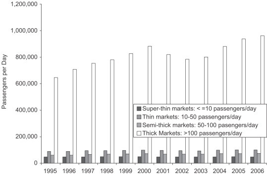
Distribution of O&D passengers in the NAS by market segment.

Despite gains in the number of markets served, passengers in thin markets fell from 93,000 in 1995 to 82,000 in 2006 with few upswings; from 1998 to 2003 and 2006. Passengers in super-thin markets, on the other hand, remained virtually constant over the same period. The average daily number of passengers in the core markets has increased significantly, from 845,000 in 1995 to 1.16 million in 2006 seemingly driven by the gains in the thick markets, up 49% over 1995 levels.

Fig. 5 shows another asymmetry underlying passenger flows, i.e., larger the passenger flow and greater the competition, the lower the average fare. Thus, those in super-thin markets, on average, pay the highest (around $240) followed by thin markets (around $197) and the semi-thick markets (around $180). Thick markets pay the lowest average one-way fare of around $163. Furthermore, average fares peak in Q1–Q2 followed by a decline in Q3–Q4 in all types of markets. Thick markets have the highest revenue share followed by thin markets. Semi-thick and super-thin markets account for around 7% of market revenue.

Fig. 5.

Average one-way fare by market types.

There are implications of using arbitrary cut-off for defining market types. Markets graduate from one category to the next. Thus, there are markets that disappear from services, for example, only to be added back during peak seasons; while others graduate upward and may be counted by the category above. The data indicate that around 5–7% of the markets fall in the former category, i.e., systematic disappearance during off-peak seasons. Given the stable characteristics of the markets as reflected by their number, passenger flow, and revenue shares, it is assumed that such changes do not fundamentally change the demand characteristics of the sample.

3. Modeling

For core markets that are fundamentally heterogeneous across different types of markets and over different seasons and years, the challenge is often how to specify a generalized quantitative framework that captures the basic relationships underlying demand. Here, we use a gravity model framework Eq. (1) to examine these relationships (Bhadra, 2003):

$$\ln (P_{\mathit{ij}})=\alpha +\beta \times \ln (f_{\mathit{ij}})+{\chi }_i\times \ln (P{I}_i)+{\chi }_j\times \ln (P{I}_j)+{\delta }_i\times \mathit{ln}({\mathrm{Population}}_i)+{\delta }_j\times \ln ({\mathrm{Population}}_j)+\phi \times \ln ({\mathrm{distance}}_{\mathit{jj}})+{\epsilon }_{\mathit{ij}},$$ (1)

where P_ij is the daily passenger flow between O&D markets, f_ij is the nominal average one-way fare between O&Ds, PI_ij is personal income in 2000 prices of the i and j communities, Population_i and Population_j represent population of markets i and j, and distance_ij is the great circle distance between i and j. The ε is the error term assumed to have a normal distribution.

O&D data are from the US DOT and is combined with economic and demographic data of the MSAs from Global Insight to construct distinct O&D market pairs between the 235 metro areas for 1995–2006. To control for quarterly variations by types of markets, the data are segmented by year, by quarter, and by types of markets giving 192 sub-samples.12 Eq. (1) is estimated for each of these sub-samples to explore the effects of structural factors, fares, and distance on the dynamics of passenger demand.

While a large population base is a sufficient condition for air travel, it is not necessary. One can easily imagine substantial travel even in remote places (e.g., Vail, Colorado in the winter) with a sparse population. Consideration of population and variables representing economic activities, either gross local area products or personal income, but not both seems reasonable in quantitative estimation.

Furthermore, there are potential problems of multicollinearity. For example, larger populations tend to be associated with higher levels of economic activities. However, in the present environment of digital communications and the Internet, this correlation may not hold for smaller communities. There is evidence indicating that the extent of this association may be loosening.13 Nonetheless, we perform the formal test of multicollinearity among the explanatory variables.14 We find the standard errors associated with the proposed explanatory variables are small and stable across sub-samples. The condition indices,15 however, appear to be larger than usually suggested. Furthermore, the variance inflation factor (VIF)—proportion of the variance of the estimates accounted for by each principal component—exceeds 10, a common measure to diagnose multicollinearity. The population variables are removed as a way to handle multicollinearity in the sub-samples.16

Table 2 presents the aggregate characteristics of the sample without yearly/quarterly and market-type classifications. It also provides Pearson correlation coefficients for the non-logarithmic variables.

Table 2.

Aggregate sample characteristics and correlations

Type	Name	Daily passengers	Average fare	Distance	Origin real income	Destination real income
Mean		30.41	229.68	1078.87	40,567.21	40,469.5
S.D.		201.01	106.79	720.92	89,009.89	88,948.21
N		1,624,579	1,624,579	1,624,579	1,624,579	1,624,579
CORR	Daily passengers	1	−0.1	−0.1	0.25	0.25
CORR	Average fare	−0.1	1	0.29	−0.06	−0.06
CORR	Distance	−0.01	0.29	1	0.05	0.05
CORR	Origin real income	0.25	−0.06	0.05	1	−0.05
CORR	Destination real income	0.25	−0.06	0.05	−0.05	1

Fig. 6 relates the explanatory power of the specified model by types of markets for 192 sub-samples (i.e., years and quarters that are represented along the horizontal axis). The demand specification appears to capture thick markets fairly well. Over 60% of the variations in the passenger in core thick markets appear to have been explained by average fares, real personal incomes of origin and destination markets, and distances between origin and destination markets. Alternatively, the specified model does not explain around 40% of the observed variations in passenger data. The explanatory powers gradually decline between 2001 and 2003, due to 9/11, the Iraq war, SARS, etc., that are outside the model. The model also tends to lose its explanatory power a little during Q1 on a systematic basis suggesting there are omitted seasonal variables.

Fig. 6.

Nature of statistical fit: Adjusted R².

The demand specification does a fairly poor job of capturing the variations in the semi-thick markets; the explained variations never exceed 10% (gray square box in Fig. 6). This clearly indicates that passenger demand considerations that are structurally (demand) framed cannot capture the observed variations in passenger flows in these markets. Many of these semi-thick markets tend to be linked fairly closely to the airline networks and other schedule requirements of the commercial airlines. Oftentimes, the provision of services is not closely linked to that supported by structural factors alone as proposed via the empirical model. The aggregate statistical performance of the thin markets appears to be closer to that of semi-thick markets; however, the explained variations in this case never exceed 25%.

On the contrary, the statistical specification tends to perform relatively well for super-thin markets with explained variations of around 36%. The trend aligns well with that of thick markets except the fact that the explained variations tend to increase a little in Q1.

While the Adjusted R ² provides important information regarding the aggregate behavior of the model, the mean squared error (MSE) of a fitted curve provides greater insights into the fit of the model to the data. For every data point, the vertical distance from the data point to the corresponding point on the fitted curve provides the error value. To eliminate the countervailing impact of positive and negative error values, the errors are then squared. Adding up the squared error values for all data points and dividing them by the number of data points, results in the MSE. Fig. 7 shows the square root of the MSE (RMSE) for the models categorized by types of markets and time (year and quarter).

Fig. 7.

Root mean squared errors.

Since Adj. R ²s are smallest for the semi-thick markets, it is somewhat surprising that, especially when compared against other sub-samples, RMSEs are smallest for this group as well. The model's explained sum of squares (SSEs) are fairly low in relation to residual sum of squares (RSSs) for these sub-samples (i.e., semi-thick) in comparison to others. In other words, sum of squares (SSTs) are disproportionately influenced by the presence of high RSSs. Thus, the ratios of SSEs and SSTs are comparatively far larger for these sub-samples resulting in generally low Adj. R ²s (adjusted by number of parameters). On the other hand, when low SSEs are weighted by number of parameters and relatively lower sample sizes (observations ranging between 820 and 1040 for these sub-samples), they result in lower RMSEs as well.

Although thick markets samples sizes are relatively few (observations ranging between 1380 and 1910), the specified model captures far more variations in dependent variable than the semi-thick markets. Consequently, the ratios of SSEs to SSTs are comparatively lower resulting in relatively better fits. Higher SSEs accompanied with relatively more observations in samples result in relatively higher RMSEs. Similar explanations hold true for super-thin (observations ranging between 25,540 and 28,220) and thin markets (between 3745 and 4550).

Over the past 12 years, both industry competition and economic growth have led to substantial expansion in the core air travel markets. Although there are other parameters, none are better represented than the fares that the average travelers paid in the markets. The average fare has a strong impact on passenger O&D flow, with a statistical significance at 99% levels of confidence for all 192 sub-samples except for six.17 The log transformation of the average fare allows interpretation of the coefficients as fare elasticities (Fig. 8 ).

Fig. 8.

Comparison of average fare elasticities.

It is evident from Fig. 8 that the demand of core markets is structurally different when evaluated at the fare elasticities. However, these results should be interpreted in conjunction with the information on average fare (Fig. 5). Thick markets appear to have elastic demand with magnitudes ranging from 1.3 (1995:Q1) to 1.8 (2006:Q2). Because fares in these markets are already relatively low, the response is likely to be relatively high due to competition. Furthermore, the elasticities began to increase starting in 2002:Q3; a trend corresponding with low cost carriers (LCCs) expanding services and more substitutes becoming available.18 Finally, the fare elasticities in these markets, shows a much larger drop in 2006:Q3–Q4 than observed in the past.

Conversely, super-thin markets face the highest fares (Fig. 5); consistent with the fact that there are very few alternatives to scheduled air travel in these smaller cities. This is corroborated by the earlier observation that the super-thin markets have indeed lost quite a few market pair services, especially in the post-9/11 period. Consequently, fare elasticities, ceteris paribus, have been found to be highly inelastic for the entire sample, especially so beginning with 2002:Q1.

While semi-thick and thin markets face fairly similar fare structures with small differences ($15–$25) across markets, elasticities behave somewhat differently (Fig. 8). Thus, for example, while a percentage fare adjustment invokes over 0.5% passenger adjustment in thin markets, it generates only a half of that in semi-thick markets. As noted earlier, many of the semi-thick markets are closely linked through the airline hub-and-spoke networks and often dominated by a single carrier and its code-sharing partners. Air travelers in many of these markets may have very few choices thus resulting in demand that is inelastic in fare. Alternatively, thin markets that are large enough to stand on their own or not part of any one dominated career's network pay a slightly higher fare but may find many more alternatives (i.e., more than twice the elasticity value vis-à-vis semi-thick markets). These markets are beginning to exhibit momentum in gaining value in fare elasticity (Fig. 8). Together, these facts perhaps indicate that the next web of airline competition is likely to take place in thin markets as opposed to semi-thick markets. Overall, the ranges of elasticities fall within the values that have been observed elsewhere (see Brons, et al. (2002) for an intra-country meta analysis).

The results show that, in general, O&D passenger travels are income-inelastic (Fig. 9, Fig. 10 ). We find that thick markets (elasticity values around 0.6) and super-thin markets (around 0.64) are similar in structure.

Fig. 9.

Origin income elasticities.

Fig. 10.

Comparison of destination income elasticities.

Super-thin and thick markets sit on opposite ends of the average real incomes. Since semi-thick markets offer far fewer alternatives, people's decisions are likely to be less sensitive to income (with estimated magnitudes <0.1). This, combined with the fact that they are also fare inelastic, tends to represent very little demand-pull from these communities. Air travel is thus a strong necessity for many of the travelers in communities that are represented by semi-thick markets. In comparison, passengers living in thin markets, with similar real incomes, have relatively more alternatives. Thus, their decisions to travel are relatively more sensitive to changes in real income than those living in semi-thick markets, resulting in almost twice in the magnitude of income elasticity coefficients, still falling within the realm of inelasticity. Following the same logic, one can also understand the rationale behind even higher income elasticities for those living in thick markets; more alternatives accompanied with higher real incomes result in relatively higher elasticity.

Similar income elasticities for super-thin markets, compared to those for thick markets, pose a challenge in explanation, especially given the fact that the levels of incomes in these markets are almost seventh of that of thick markets. To understand this finding, one has to take into account both the spatio-locations and income distributions in the super-thin markets. For most cases, these markets are constituted by the suburban and peripheral areas that are outside the main urban centers of the MSAs.19 Generally speaking, these areas are scattered in the US. However, the locations of their employment and the accounting of their contributions make these smaller communities demonstrate economic behaviors resembling more like larger communities. Thus, while passengers in these small communities are restricted by access to scheduled air travels, their decisions to travel by air are influenced more by their incomes which override the access constraints, thus resulting in elasticities that are closer to those for thick markets.

The estimates indicate that while thick markets demonstrated a slight decline in the magnitude of income elasticity following the economic slowdown of spring 2001, super-thin markets did not. Relatively higher income elasticities combined with very inelastic fare elasticities (Fig. 8) for super-thin markets are potentially attractive to providers exploring alternative networks. The decision of air taxi providers using very light jets to serve many of these communities (e.g., DayJet) perhaps indicates such potential. Larger size of the markets combined with intense competitive forces make it harder to draw such attraction to thick markets. Thus, these super-thin markets that are relatively responsive to income changes and irresponsive to fare changes are indeed potentially attractive markets for introduction of new lines of air-travel products. The high cost of operating scheduled air carrier network makes servicing these smaller markets difficult.

The magnitude of income elasticities with respect to destination communities20 and their structure are essentially similar to those of origin communities (Fig. 10).

Distance between O&D communities, when controlled for fares, may reveal important insights into understanding the structure of the O&D demand. In Fig. 11 , we report these elasticities (vertical axis) by market types and year and quarter (horizontal axis).21

Fig. 11.

Comparison of distance elasticities.

Overall, O&D travels from these markets do not necessarily invoke proportional increases in passenger flow.22 Controlling for fares, this would imply that there are limited demand responses among the travelers for further distanced market pair services. While thick and thin markets demonstrated somewhat upward mobility and thus greater responses (within the range of inelasticity) in the distance elasticities, especially after 2001:Q3, it remains virtually constant for the other two markets. These results compare well with our earlier discussion on gaining new market pair services by market categories. If these trends continue in the future, thick and thin markets would indeed have greater opportunities for newer and distant city pair services than semi-thick and super-thin market pair services.

4. Conclusions

The paper has provided an analysis of the fundamental structures and dynamics of the O&D or core air travel markets in the US using quarterly data covering 1995–2006. Services provided demonstrate strong seasonality that is not so pronounced in passenger levels. Despite the industry consolidating its network following the events of 9/11, passenger flows between O&D markets have exhibited strong growth in recent years. When segmented by types of markets, we found that while super-thin markets lost service, other market segments gained service. A majority of passengers fly in the thick markets that account for only a small portion of the markets and the demand has continued to grow over time. Relatively, many fewer passengers fly in the thin and super-thin markets, but they account for a substantial portion of the markets.

To capture the basic demand drivers underlying the O&D market pairs, an empirical framework is offered that formalizes the relationship between passenger flow to average fares, incomes of these core communities, and market distances between communities. We apply this framework on the 192 sub-samples that have been segmented by year, quarter, and by types of markets. The overall fits indicate that thick markets and super-thin markets have relatively better fit to the data. Using this overall empirical framework, we found that while thick markets exhibited relatively elastic demand with respect to changes in fares, other communities are decisively inelastic. In particular, semi-thick and super-thin markets have been found to have highly inelastic demand with respect to changes in average fares. Income elasticities (both origin and destination), on the other hand, are altogether inelastic although thick and super-thin markets tend to have relatively larger quotients than semi-thick and thin markets. Finally, distance elasticities have been found to be inelastic. While thick and thin markets share common properties and show an upward trend over time, passenger flows in semi-thick and super-thin markets remained decisively distance-inelastic. Empirical estimates seem to capture and align well with the events and adjustments that have been experienced during the time series we examined.

References

- Bhadra D. Demand for air travel in the United States: bottom-up econometric estimation and implications for O&D forecasts by O&D pairs. Journal of Air Transportation. 2003;8:19–56. [Google Scholar]
- Bhadra D. Air travel in small communities: an econometric framework and results. Journal of the Transportation Research Forum. 2004;43:19–37. [Google Scholar]
- Bhadra D., Hechtman D. Determinants of airport hubbing in the US: an econometric framework. Public Works Management and Policy. 2004;9:26–50. [Google Scholar]
- Borenstein S., Rose N. The impact of bankruptcy on airline service levels. American Economic Review; Papers and Proceedings. 2003;93:415–419. [Google Scholar]
- Brons M., Pels E., Nijkamp P., Rietveld P. Price elasticities of demand for passenger air travel: a meta analysis. Journal of Air Transport Management. 2002;8:165–175. [Google Scholar]
- Brueckner J.K., Zhang Y. A model of scheduling in airline networks: how a hub-and-spoke system affects flight frequency, fares and welfare. Journal of Transport Economics and Policy. 2001;35:195–222. [Google Scholar]
- Button K., Lall S., Stough R., Trice M. High-technology employment and hub airports. Journal of Air Transport Management. 1999;5:53–59. [Google Scholar]
- Federal Aviation Administration, 2007a. Aerospace forecasts 2007–2020, US Department of Transportation, Washington, DC. 〈http://www.faa.gov/data_statistics/aviation/aerospace_forecasts/2007-2020/〉.
- Federal Aviation Administration, 2007b. National plan of integrated airport systems (2007–2011), US DOT, Washington DC. 〈http://www.faa.gov/airports_airtraffic/airports/planning_capacity/npias/reports/media/2007/npias_2007_narrative.pdfl〉.
- Forman, C., Goldfarb, A., Greenstein S., 2003. How did location affect adoption of the commercial Internet? Global village, urban density, and industry composition. NBER Working Paper No. 9979.
- Glaeser E.L. Are cities dying? The Journal of Economic Perspectives. 1998;12:139–160. [Google Scholar]
- Government Accountability Office, 2002. Commercial aviation: air service trends at small communities, report to Congressional requesters, GAO. Report No. GAO-02-432. Washington, DC.
- GRA, Inc., 2003. Alternate airports study. Final Report prepared for the Office of the Assistant Secretary for Transport Policy, US DOT, Washington, DC.
- Irwin M.D., Kasarda J.D. Air passenger linkages and employment growth in US metropolitan areas. American Sociological Review. 1991;56:524–537. [Google Scholar]
- Ito H., Lee D. Assessing the impact of the September 11 terrorist attacks on US airline demand. Journal of Economics and Business. 2004;57:79–95. doi: 10.1016/j.jeconbus.2004.06.003. [DOI] [PMC free article] [PubMed] [Google Scholar]
- Lee D. Concentration and price trends in the US domestic airline industry. Journal of Air Transport Management. 2003;9:91–101. [Google Scholar]
- Windle R., Dresner M. Competitive responses to low cost carrier entry. Transportation Research E. 1999;35:59–75. [Google Scholar]