

Abstract
Different from prior studies which concentrate on the unidirectional impact of industry leading, this study examines the bi-directional dynamical causal relation between industry returns and stock market returns by considering multiple structural breaks for ten major eastern and southern Asia countries. Our results show that finance and consumer service industry returns have significant power in explaining the movements of market returns. Further, we apply logit regressions to explore the determinants of the leading hypotheses and find exchange rate and interest rate are important in explaining the industry–market nexus. In a developed market the industry and the market have feedback relations, but in a highly controlled economy the influence from the stock market dominates.
Keywords: Industry, Stock market returns, Granger causality, Structural breaks, Logit model
1. Introduction
Industry-level data provides us the source of country economic growth to its industry origins (Jorgenson & Nomura, 2005). As a large body of research concentrates on the unidirectional relationship between industry and stock market returns and produces divergent findings, little of the studies discuss about the bi-relationships. For instance, Tessitore and Usmen (2005) compare different industries and find that financials and telecommunications are the dominant industries in explaining stock market returns. Hong, Torous, and Valkanov (2007) verify that industries can lead the stock market, because the returns of industry portfolios that are informative about macroeconomic fundamentals are shown to lead the aggregate market. Tsuji (2012) finds all U.S. industries strongly forecast one-month-ahead small-minus-big factor returns.
Using Granger causality tests and generalized impulse response functions (hereafter, GIRF), we address these concerns of the dynamic relationships between industry returns and market returns by a rigorous time-series analysis. This paper investigates the dynamic linkages between industry and stock market returns from a broader perspective through four hypotheses: (i) industry leading hypothesis: Industry returns exert a unidirectional leading effect on market returns. The hypothesis may be sustained by government support for a specific industry. (ii) market leading hypothesis: Industry returns are determined by market returns, i.e., rising or declining market returns precede the change in industry returns. (iii) feedback hypothesis: There exists a bi-directional causal relation between industry and market returns, meaning that industry and market returns are determined jointly (iv) neutrality hypotheses: No causal relation exists between industry and market returns, meaning that industry returns are not correlated with market returns. We further examine the factors determining the presence of these hypotheses such as GDP growth rate, exports, inflation rate, exchange rate, interest rate, etc.
Studies have documented the dominance of different industries on the overall stock market returns. The original study by Roll (1992) points out that the capital goods sector is essential for Germany, whereas basic goods sector is important for such producers as South Africa, yet negative for raw material importers like Hong Kong. This implies that industry effects are restrained by country resources and amplified by national advantages. Griffin and Karolyi (1998) reveal that internationally-traded goods industries explain a relatively large proportion of the variation in returns, compared with non-internationally-traded goods industries. Wang, Lee, and Huang (2003) indicate that the influence of the information technology (IT) industry on the stock market apparently dominates that of traditional industries. Tessitore and Usmen (2005) demonstrate that the importance of the IT industry on returns has diminished, and the prominent contributors to industry effects are financials and telecommunications. Thus, the result of the industry returns-stock market returns nexus is still inconclusive.
This paper offers some new features that are not necessarily shared by the aforementioned studies. First, whereas Hong et al. (2007) analyze OECD countries and obtain similar results among them for large and developed markets, we instead consider ten adjacent eastern and southern Asia markets (one developed and nine emerging economies) to explore if the industry-market return nexus is different within similar cultures and economies, which could decrease the considerable divergence among different capital markets. The economic successes of several Asian economies and their increasingly important roles in the global financial market have lately motivated several studies (Ito, 2006, Kang and Yoon, 2006, Lee et al., 2013a). Most of the prior related literature assesses major developed countries, except Wang et al. (2003). The study of the industry-market nexus focusing on 10 eastern and southern Asia countries has important implications for international investors as the area is now an important emerging market.
Second, the majority of the related studies use cross-sectional analyses (Hong et al., 2007, Roll, 1992, Serra, 2000), which are useful particularly when these relationships are stable over time. If the relationship is not necessarily stable, but instead evolves over time as several economists argue, then cross-sectional analyses may provide a limited depiction about the relationship. Time-series analyses over the debate on the dynamic associations of the industry and market returns from an alternative perspective are still scarce. To complement recent studies, we focus on time-series analyses concerning the relative importance of the industry-based versus market-based debate.
Third, our sample period covers 2001–2010, during which there were several significant exogenous shocks: severe acute respiratory syndrome (SARS) outbreak (2003), the U.S. subprime mortgage crisis (2005–2006), Iraq War (2003–2008), and the global financial crises (2007–2010). We consider the effect of structural breaks in the stock returns, because the stock market is closely correlated with an economic system, and the impact of external factors is inescapable and should attract attention. Neglecting structural break problems makes it hard to find out whether or not parameters are unstable within each of the sub-periods (Lee, 2013, Lee and Chang, 2005) – that is, without considering a structural break, the causal relationship may not be clearly identified due to the effect of unusual economic events.
Finally, in this paper we conduct both cross-country and cross-industry comparisons by examining different data intervals, different data frequencies, and the effect of both trading activity and the potential business cycle, as well as perform an out-of-sample performance test to compare the difference between historical mean returns and returns based on the predicted model. Further, we execute the logit regression analysis to identify the possible factors influencing the dominance of different hypotheses.
Using daily data that cover 2001/1/1 to 2010/12/31, our findings indicate that the causal relation between industry and market returns differs across industries as well as countries, implying that alternative hypotheses co-exist in stock markets of eastern and southern Asia. For instance, the industry leading hypothesis is supported in the following industries and countries: basic materials in China; consumer services in India, Japan, and Malaysia; financial industry in South Korea, Taiwan, and Thailand; health care in Singapore and Taiwan; oil and gas in Thailand; and technology in Malaysia. This suggests that returns of these industries could be used to predict the overall market returns in the respective countries, possibly because of government support for specific industries or due to some industries making up a substantial proportion of the overall stock market values. And, a growth revival can be spotted in the above mentioned industries.
Our findings also present the importance of market characteristics from different countries. For instance, in Japan, the only developed market in the sample, we observe a significant bi-directional causality between market and industry returns, i.e., the feedback hypothesis, in six out of the ten included industries as compared to Indonesia where the market leading hypothesis is supported in seven out of the ten industries. An obvious difference is identified between the two countries. That is, private enterprises in Japan are major actors in the market and the government exerts little intervention; in Indonesia, however, state-owned enterprises play a prominent role in the economy. The results imply that in a freely developed market the industry and the market affect each other, but in a highly controlled environment the influence from the market side dominates.
After identifying the presence of alternative hypotheses, in a logit model analysis, we find that the industry leading hypothesis is positively correlated with government support, but negatively correlated with exports, oil price, the exchange rate, and the interest rate. The market leading hypothesis is negatively correlated with change in GDP, but positively correlated with the interest rate, the exchange rate, and expected growth. The exchange rate and interest rate are crucial factors that affect the hypotheses simultaneously. The importance of former should be associated with the high dependence on exporting in eastern and southern Asia. Our findings are helpful for investors and financial analysts focusing on these stock markets when formulating investment strategies.
The study is organized as follows. Section 2 describes the data and methodology. Section 3 discusses the empirical findings and the implications of the results. Section 4 provides robustness checks. Section 5 presents the conclusions.
2. Data and methodology
2.1. Data
This study uses daily data from 2001/01/01 to 2010/12/31 for ten adjacent eastern and southern Asia countries (China, Hong Kong, India, Indonesia, Japan, South Korea, Malaysia, Singapore, Taiwan, and Thailand). To examine the impact of the long-, intermediate-, and short-term industry returns on market returns, we test the data span covering 10 years, 3 years, and the latest 1 year intervals. We apply the industry classification benchmark (IBC) to segregate markets into ten major industries: basic materials (MATS), consumer goods (GDS), consumer services (SVS), financials (FIN), health care (HEA), industrials (INDU), oil & gas (OIL), technology (TECH), telecommunications (TELE), and utilities (UTIL). The industry indices and market indices in US dollars are from Datastream. We retrieve data for explanatory variables applying logit model analysis (i.e., exports, inflation rate, the percentage change of the domestic price of oil, exchange rate, percentage change in GDP, and the effective interest rate) from World Development Indicators compiled by the World Bank. The control variable (trading activity)1 and explanatory variable – expected growth of real GDP from Datastream. Industry size is computed by the percentage of industry market values obtained from Datastream. The business cycles of Japan and Taiwan are from Cabinet Office of Japan (www.esri.cao.go.jp) and Council for Economic Planning and Development of Taiwan (www.cepd.gov.tw), respectively.
2.2. Granger causality test and general impulse response analysis
Following Torres and Vela (2003), this article employs the Granger causality test to examine the causal relationship between industry returns and stock market returns. Causality in the Granger (1969) sense is inferred when values of a variable, x t (industry returns), have explanatory power in a regression of y t (stock market returns) on the lagged values of x t and y t. If the lagged values of x t have no explanatory power for any other variable in the system, then y t is viewed as weakly exogenous to the system. The baseline VAR model estimates the following two equations:
| (1) |
| (2) |
where p and q are the number of the optimum lag length, and μ t and v t are the random error terms. Since there are ten major industries in each country, we have a total of 100 pairs of Granger causality tests. Optimum lag lengths are determined empirically by the Schwarz Information Criterion (SIC).
Impulse responses present the impact of one standard deviation shock or the innovation of one variable on the current and future values of another variable. A major difficulty with traditional IRF analysis is that the technique involves a prior orthogonalization of shocks based on a Choleski decomposition of the matrix of variance innovations. This decomposition is not unique in essence, this means that the results of traditional analysis is predetermined by the manner in which the system variables are ordered. In literatures in which the fundamental issue involves causal ordering this is clearly problematic (Raju & Melo, 2003).
Thus, applying the GIRF method of Pesaran and Shin (1998), we examine the transmission mechanism between industry returns and market returns as it does not depend upon the ordering of the variables in the VAR. A key feature of GIRF is that the generalized responses are invariant to any re-ordering of variables in the system, which provides more robust results than the orthogonalized method. Another important feature is that, because orthogonality is not imposed, the GIRF allows for a meaningful interpretation of the initial response of each variable to shocks originating from any of the other variables. Following Gelain (2010) and Lee, Huang, and Yin (2013b), GIRFs are employed to trace the time paths of all variables in the system.
2.3. VAR model with multiple structural changes
Conventional Granger causality tests based on standard VAR tests may not be appropriate when the series contain structural breaks. To compensate for such a problem, we examine if potential multiple structural breaks occurred within each sample period in the robustness test during the subprime mortgage and Asian financial crises. We utilize the estimating and testing procedures of multiple structural changes in the multivariate regressions proposed by Qu and Perron (2007) to examine whether structural breaks exist in the stock markets of the ten countries. If a structural break exists over a sample period, then an empirical estimation using the entire sample will cease to provide reliable results and hypothesis testing will no longer be valid (Kim, Leatham, & Bessler, 2007).
Assume the number of structural changes in the system is m. The break dates take place at T 1, …, T m, respectively, and the convention is used whereby T 0 = 1 and T m+1 = T1. Subscript j denotes a regime and subscript t denotes a temporal observation . Consider the following model:
| (3) |
where y1,t shows stock market returns at time t, y 2,t presents the industry returns at time t, u 1,t and u 2,t are respective error terms with mean 0 and covariance matrix Σj for T j−1 + 1 ≤ t ≤ T j, and β i,j, i = 1, …, 6, are coefficients to be estimated.
We rewrite Eq. (3) in the following form:
| (4) |
where , , S is an identity matrix of dimensions (6 × 6), , and . To ease notation, define the (6 × 2) matrix x t by so that Eq. (4) becomes:
| (5) |
for .
It is useful to express the model in an alternative form. Let be the 2T vector of dependent variables, let , and let the (2T × 6) matrix of regressors be . For a given partition of the sample with the breaks T 1, …, T m, define the block partition of the matrix X as the matrix , where is the subset of X corresponding to observations in regime j. The subvector U j of U is defined in a similar way. The regression system (5) can now be expressed as .
Qu and Perron (2007) derive the estimation and inference procedures by utilizing the restricted quasi-maximum likelihood. Conditional on a given partition of the sample , the aim is to obtain values of that maximize the quasi-likelihood function subject to a set of r restrictions of the form:
| (6) |
where , , and g(·) is an r − dimensional vector. The model allows within- and cross-equation restrictions, and for each case within or across regimes. For the estimation, Qu and Perron (2007) propose the dynamic programming algorithm advocated by Hawkins (1976) and Bai and Perron (2003). For the test of structural changes, we consider a likelihood ratio test for the null hypothesis of no change in any of the coefficients versus an alternative hypothesis with a pre-specified number of changes, say m.
We briefly describe the procedure as follows. Under the null hypothesis of no structural change, the estimates of coefficients and variances are the values and that jointly solve the system of equations:
| (7) |
| (8) |
and the value of the log-likelihood function is , where n denotes the number of equations in the system.
For a given partition , the class of models can be estimated by quasi-maximum likelihood using the appropriate restrictions. Denote the log-likelihood value by . The test is the maximum value of the likelihood ratio over the admissible partitions:
| (9) |
Here, the estimates are the quasi-maximum likelihood estimation obtained by considering only those partitions in the set of permissible partitions. The exact form of the log-likelihood value and the estimates of the coefficients for some certain cases are presented in Qu and Perron (2007).
3. Empirical results
3.1. Data description
Table A1 in Appendix summarize descriptive statistics of the market and industry returns for ten sampling countries. Data on TECH in Indonesia and UTIL in both Taiwan and Singapore are not available. We find that all of the daily returns averages are positive and range from 0.0000 for Japan to 0.0009 for Indonesia, with 0.0008 for China. Consistent with the information asymmetry theory, the Japanese market is the most developed compared to the others, where investors there are more informed, and thus any opportunity for arbitrage is limited. South Korea has the highest standard deviation of 0.0214. The Jarque–Bera tests strongly reject normality for all the sample markets, and thus using OLS may obtain misleading results. Among the ten industries, the three with higher returns are MATS, GDS, and OIL in our sample, which are contrary to Yang, Tapon, and Sun (2006) who document that TECH had the highest return during the IT boom period of 1998 to 2002. MATS having the highest average return (0.00069) is consistent with Tessitore and Usmen (2005) who find that MATS dominated during 2001–2010 using UK and U.S. samples.
3.2. Granger causality results
The results of Granger causality tests in Table 1 show that market returns are affected by past movements of MATS returns in China; by SVS in India, Japan, and Malaysia; by FIN in South Korea, Taiwan, and Thailand; by TECH in Malaysia; by HEA in Singapore and Taiwan; and by OIL in Thailand. We find a new trend that SVS leads market returns.
Table 1.
| Country | MATS | GDS | SVS | FIN | HEA | INDU | OIL | TECH | TELE | UTIL | |
|---|---|---|---|---|---|---|---|---|---|---|---|
| China | (a) | 7.884** (0.005) | 9.791** (0.002) | 0.914 (0.339) | 0.614 (0.433) | 12.692** (0.000) | 1.309 (0.253) | 0.287 (0.593) | 15.073** (0.000) | 5.532* (0.019) | 0.104 (0.747) |
| (b) | 1.203 (0.273) | 6.273* (0.012) | 2.656 (0.103) | 3.768 (0.052) | 8.205** (0.004) | 1.385 (0.239) | 0.295 (0.587) | 15.882** (0.000) | 8.989** (0.003) | 4.477* (0.035) | |
| Direction of Causality | Market ← MATS, GDS, HEA, TECH, TELE Market → GDS, HEA, TECH, TELE, UTIL |
||||||||||
| Hong Kong | (a) | 3.050 (0.081) | 0.863 (0.353) | 2.797 (0.095) | 0.505 (0.477) | 0.431 (0.512) | 0.249 (0.618) | 1.137 (0.287) | 1.465 (0.226) | 0.087 (0.768) | 4.449* (0.035) |
| (b) | 1.076 (0.300) | 0.073 (0.787) | 0.943 (0.332) | 5.728* (0.017) | 3.234 (0.072) | 0.575 (0.448) | 6.205* (0.013) | 0.830 (0.362) | 10.387** (0.001) | 49.194** (0.000) | |
| Direction of Causality | Market ← UTIL Market → FIN, OIL, TELE, UTIL |
||||||||||
| India | (a) | 0.771 (0.380) | 3.693 (0.055) | 7.873** (0.005) | 1.965 (0.161) | 13.670** (0.000) | 3.209 (0.073) | 0.021 (0.886) | 3.618 (0.057) | 1.892 (0.169) | 0.988 (0.320) |
| (b) | 2.615 (0.106) | 6.686** (0.010) | 2.549 (0.111) | 0.012 (0.911) | 7.520** (0.006) | 16.494** (0.000) | 6.636* (0.010) | 26.404** (0.000) | 0.533 (0.466) | 3.502 (0.061) | |
| Direction of Causality | Market ← SVS, HEA, Market → GDS, HEA, INDU, OIL, TECH |
||||||||||
| Indonesia | (a) | 0.084 (0.772) | 0.089 (0.766) | 0.077 (0.781) | 0.658 (0.417) | 0.196 (0.658) | 0.733 (0.392) | 0.050 (0.823) | N/A | 2.473 (0.085) | 2.667 (0.103) |
| (b) | 4.135* (0.042) | 21.087** (0.000) | 20.944** (0.000) | 27.451** (0.000) | 3.103 (0.078) | 12.134** (0.001) | 0.335 (0.563) | N/A | 3.651* (0.026) | 6.998** (0.008) | |
| Direction of Causality | Market ← Market → MATS, GDS, SVS, FIN, INDU, TELE, UTIL |
||||||||||
| Japan | (a) | 3.968* (0.047) | 0.510 (0.600) | 11.016** (0.001) | 4.783* (0.029) | 17.702** (0.000) | 3.219* (0.040) | 0.010 (0.922) | 7.888** (0.005) | 3.484 (0.062) | 23.569** (0.000) |
| (b) | 7.812** (0.005) | 14.232** (0.000) | 0.646 (0.422) | 20.375** (0.000) | 5.953** (0.003) | 16.068** (0.000) | 8.884** (0.003) | 37.433** (0.000) | 2.456 (0.117) | 18.488** (0.000) | |
| Direction of Causality | Market ← MATS, SVS, FIN, HEA, INDU, TECH, UTIL Market → MATS, GDS, FIN, HEA, INDU, OIL, TECH, UTIL |
||||||||||
| Country | MATS | GDS | SVS | FIN | HEA | INDU | OIL | TECH | TELE | UTIL | |
|---|---|---|---|---|---|---|---|---|---|---|---|
| South Korea | (a) | 3.696 (0.055) | 0.238 (0.626) | 1.200 (0.273) | 4.635* (0.031) | 0.173 (0.678) | 3.076 (0.080) | 0.357 (0.550) | 0.447 (0.504) | 7.016** (0.001) | 1.019 (0.313) |
| (b) | 6.752** (0.009) | 0.416 (0.519) | 0.002 (0.962) | 0.120 (0.730) | 0.686 (0.408) | 0.020 (0.888) | 3.682 (0.055) | 0.339 (0.560) | 24.813** (0.000) | 3.220 (0.073) | |
| Direction of Causality | Market ← FIN, TELE Market → MATS, TELE |
||||||||||
| Malaysia | (a) | 0.019 (0.891) | 2.061 (0.151) | 22.857** (0.000) | 0.385 (0.535) | 0.024 (0.878) | 7.877** (0.005) | 0.586 (0.444) | 12.978** (0.000) | 3.724 (0.054) | 3.015 (0.083) |
| (b) | 6.795** (0.009) | 34.018** (0.000) | 0.009 (0.927) | 12.048** (0.001) | 8.192** (0.004) | 25.808** (0.000) | 15.465** (0.000) | 0.604 (0.437) | 3.559 (0.059) | 23.607** (0.000) | |
| Direction of Causality | Market ← SVS, INDU, TECH Market → MATS, GDS, FIN, HEA, INDU, OIL, UTIL |
||||||||||
| Singapore | (a) | 0.411 (0.522) | 2.375 (0.123) | 0.866 (0.352) | 0.001 (0.974) | 5.645* (0.018) | 0.104 (0.747) | 0.523 (0.470) | 0.001 (0.969) | 1.046 (0.306) | N/A |
| (b) | 4.257* (0.039) | 6.586* (0.010) | 4.621* (0.032) | 1.113 (0.292) | 0.776 (0.379) | 0.005 (0.943) | 0.514 (0.474) | 0.012 (0.912) | 7.407** (0.007) | N/A | |
| Direction of Causality | Market ← HEA Market → MATS, GDS, SVS, TELE |
||||||||||
| Taiwan | (a) | 1.078 (0.299) | 1.301 (0.254) | 0.210 (0.647) | 8.930** (0.003) | 5.445* (0.020) | 0.174 (0.677) | 0.059 (0.808) | 6.342* (0.012) | 0.172 (0.679) | N/A |
| (b) | 0.323 (0.570) | 2.325 (0.127) | 0.071 (0.790) | 2.454 (0.117) | 3.041 (0.081) | 0.262 (0.609) | 0.284 (0.594) | 9.361** (0.002) | 14.430** (0.000) | N/A | |
| Direction of Causality | Market ← FIN, HEA, TECH Market → TECH, TELE |
||||||||||
| Thailand | (a) | 0.242 (0.623) | 0.002 (0.966) | 0.546 (0.460) | 5.291* (0.022) | 0.884 (0.347) | 0.083 (0.774) | 5.873* (0.015) | 3.455 (0.063) | 0.236 (0.627) | 1.185 (0.276) |
| (b) | 8.457** (0.004) | 1.611 (0.205) | 1.036 (0.309) | 0.641 (0.423) | 3.591 (0.058) | 4.274 (0.039) | 1.438 (0.231) | 3.438 (0.064) | 0.508 (0.476) | 10.899** (0.001) | |
| Direction of Causality | Market ← FIN, OIL Market → MATS, INDU, UTIL |
||||||||||
Notes: Figures denote F statistic. p-values are given in parentheses. ** and * indicate that the parameter estimates are significant at the 1% and 5% levels, respectively. “→ (←)” means market returns (industry returns) Granger cause industry returns (market returns). N/A denotes data are not available.
(a)Null hypothesis: Industry returns do not Granger cause market returns.
(b)Null hypothesis: Market returns do not Granger cause industry returns.
We summarize the results of the Granger-causality test in Panel A of Table 2 , which shows that a leading relationship between industry and market returns varies across countries. The results demonstrate that the four hypotheses we intend to examine appear to co-exist in the selected eastern and southern Asia countries, possibly because of differences in country environments or government industry policies. Our results suggest that focusing attention only on a unidirectional relation from industry return to market return may be incomplete and thus does not present the whole picture on the nexus, particularly in a cross-country investigation.
Table 2.
Summary of Granger causality test results between industry and market daily returns (Eqs. (1), (2)).
| Country | MATS | GDS | SVS | FIN | HEA | INDU | OIL | TECH | TELE | UTIL |
|---|---|---|---|---|---|---|---|---|---|---|
| Panel A. US currency | ||||||||||
| China | ← | ⇔ | ⇔ | ⇔ | ⇔ | → | ||||
| Hong Kong | → | → | → | ⇔ | ||||||
| India | → | ← | ⇔ | → | → | → | ||||
| Indonesia | → | → | → | → | → | NA | → | → | ||
| Japan | ⇔ | → | ← | ⇔ | ⇔ | ⇔ | → | ⇔ | ⇔ | |
| South Korea | → | ← | → | ⇔ | ||||||
| Malaysia | → | → | ← | → | → | ⇔ | → | ← | → | |
| Singapore | → | → | → | ← | → | NA | ||||
| Taiwan | ← | ← | ⇔ | → | NA | |||||
| Thailand | → | ← | → | ← | → | |||||
| Panel B. Local currency (Robustness check) | ||||||||||
| China | ← | ⇔ | ⇔ | ⇔ | ⇔ | → | ||||
| Hong Kong | → | → | → | ⇔ | ||||||
| India | ← | ← | ⇔ | ⇔ | → | ⇔ | ||||
| Indonesia | → | → | → | → | → | N/A | → | |||
| Japan | → | → | ⇔ | → | → | → | ||||
| South Korea | → | → | → | |||||||
| Malaysia | → | ← | → | → | ← | ← | → | → | ||
| Singapore | → | ← | ← | ⇔ | → | |||||
| Taiwan | ← | ← | ⇔ | → | N/A | |||||
| Thailand | → | ← | ← | → | ||||||
| Panel C. Control trading activity (Robustness check) | ||||||||||
| China | ← | ⇔ | ⇔ | ⇔ | ⇔ | → | ||||
| Hong Kong | → | → | → | ⇔ | ||||||
| India | → | ← | ⇔ | → | → | ⇔ | ||||
| Indonesia | → | → | → | → | N/A | → | ||||
| Japan | ⇔ | → | ← | ⇔ | ⇔ | ⇔ | → | ⇔ | ⇔ | |
| South Korea | → | ← | ⇔ | |||||||
| Malaysia | → | → | ← | → | → | ⇔ | → | → | ||
| Singapore | → | → | → | ← | N/A | |||||
| Taiwan | ⇔ | ⇔ | → | N/A | ||||||
| Thailand | → | ← | → | ← | → | |||||
Notes: “→” means market returns Granger cause industry returns, supporting the market leading hypothesis. “←” means industry returns Granger cause market returns, supporting the industry leading hypothesis. “⇔” means market returns and industry returns Granger cause each other, supporting the feedback hypothesis. Empty cell means no causality between industry and market returns, supporting the neutrality hypothesis. N/A denotes data are not available.
To check if the results above are robust, we use an alternative currency measure and control for the effect of trading activity. Panel B using local currency returns shows the findings on the industry leading hypothesis with US currency measure still hold in eight out of eleven industry-leading industries in the local currency. The difference is unavoidable, because the change in exchange rates across countries is different due to various trade conditions, and thus evaluating the return in a different currency base will cause differences. We concentrate on the results obtained using the US dollar return series for two reasons. First, a common currency across the ten sampling markets allows us to compare the results easily. Results in terms of US dollar measure are especially relevant to international investors (Chen, Firth, & Rui, 2002). Second, when returns of indices are expressed in a local currency, part of the index’ return volatility is induced by monetary phenomena such as changes in anticipated and actual inflation rates. Historically, inflation emerged as the biggest macroeconomic challenge confronting developing Asia during 2007–2008 (Jongwanich & Park, 2009), leading results to interpretation problems in using returns denominated in the local currency. In Panel C of Table 2, we control trading activity by including trading activity as an independent variable into the empirical model to evaluate its impact on industry-market returns, which is a manner commonly adopted in previous studies (i.e., Chen et al., 2012, Wang, 2010). The results in Panel C shows still hold in eight out of eleven industry-leading industries in controlling for trading activity, suggesting that trading activity does not substantially affect the industry leading relation here. In the past, nations use tariffs, exchange controls, quotas, restraints, and competitive devaluation of currencies, as instruments to control trading activity (MaPherson, 1995). We attribute the difference results between US dollar and local currency measures for inflation and monetary policy, and the difference with and without controlling for trading activity for government's regulation to influence specific industry.
3.3. Determinants of the causal relation
To examine what affects the relationship between industry and market returns, we perform a logit regression analysis with a leading dummy variable equal to one if the market (industry) return leads the industry (market) return or if a bidirectional relation exists, and zero otherwise. Vassalou (2003) suggests that news related to future GDP growth along with the market factor can explain the cross-section of equity returns as well as the Fama-French model. Ritter (2005) find the salient correlation between real stock returns and per capital GDP growth. Chang, McAleer, and Tansuchat (2013) mention that fluctuations in oil prices are likely to have significant effect on the production sector as with every production sector relying heavily on oil as an energy source. Stock returns are negatively related to inflation rate (Geske and Roll, 1983, Kaul, 1987). Exchange rate fluctuations can have a significant impact on trade volume as well as affect the value of firms that are involved in international business. Wang and Mayes (2012) state that interest rate has an effect on stock prices. Keim (1983) provides evidence on the time series behavior of the size effect. We are the first, to our knowledge, to address the impact of industry size on industry returns. Johnson and Mitton (2003) show that firm gains official government support to increases in stock prices. Bekaert, Harvey, and Lundblad (2003) demonstrate that equity market liberalizations lead to important changes in both the financial and real sectors as the economy becomes integrated into world capital markets. Lin and Shiu (2003) find that foreign investors strongly prefer firms with high export ratios which they are more familiar on account of their higher foreign sales. Until now, the relationship between macro-level export and industry returns is seldom discussed.
After reviewing the literature regarding factors impacting industry and/or market returns, several variables are used: expected growth of real GDP, exports, inflation rate, the percentage change of the domestic price of oil, exchange rate, the change in GDP, the effective interest rate, and industry size measured by the market value of the industry. Government support is a dummy variable that equals 1 if described government support has appeared in the country industry report, and 0 otherwise. Liberalization is cross-listing or country fund listing from Bekaert and Urias (1996) and Patro (2002).
Table 3 shows the results of the logit regression models, in which the exchange rate and interest rate are the two most prominent factors affecting industry-market returns nexus, and the effect is different from the two alternative hypotheses. For the market leading hypothesis, expected growth and change in GDP have significant influences, while export, oil price, and government support are important for the industry leading hypothesis. The exchange rate being relevant with respect to the two alternative hypotheses should correlate with the high dependence on exporting by sampling Asian countries. Government support determining whether industry returns lead market returns may be correlated with government policies for specific industries. An in-depth discussion about these determinants is not pursued here due to space limitation, but may be a topic worthy of further investigation in the future.
Table 3.
Logit model on determinants of the market-industry leading relationship.
| Independent variables | Market leads industry |
Industry leads market |
|---|---|---|
| (i) | (ii) | |
| Growth | 0.1312** | 0.1519 |
| (0.0520) | (0.0990) | |
| Export | −1.40e-10 | −1.31e-08*** |
| (7.62e-10) | (2.68e-09) | |
| Inflation | 0.0292 | −0.1306 |
| (0.0405) | (0.0796) | |
| Oil_Price | −0.0003 | −0.0016*** |
| (0.0002) | (0.0005) | |
| Exchange_Rate | 0.0001*** | −0.0029*** |
| (4.24e-05) | (0.0005) | |
| GDP | −0.0054** | 0.0013 |
| (0.0021) | (0.0028) | |
| Interest_Rate | 0.1580** | −0.2736** |
| (0.0721) | (0.1380) | |
| Size | 2.83e-08 | 7.15e-07 |
| (3.00e-07) | (6.12e-07) | |
| Gov_support | −0.3612 | 6.7020*** |
| (0.2605) | (0.7949) | |
| Lib | −0.0463 | −0.0517 |
| (0.0342) | (0.0484) | |
| Constant | 2.8979 | 4.5375 |
| (3.0683) | (4.2477) | |
| Pseudo R2 | 0.0807 | 0.4683 |
Notes: This table presents the logit regression results. Model (i) tests the factors that affect the market Granger causing the industry; Model (ii) tests the factors that affect the industry Granger causing the market. In Model (i), the dependent variable is a dummy that equals 1 if the market returns Granger cause industry returns, and 0 otherwise. In Model (ii), the dependent variable is a dummy that equals 1 if the industry returns Granger cause market returns and 0 otherwise. Growth means expected growth of real GDP. Exports denote annual exports. Inflation is the annual inflation rate. Oil price is the percentage change of the domestic price of oil. Exchange_rate is the local currency per US dollar. GDP is percentage change in GDP. Interest rate is the effective interest rate. Size is the market value of the industry. Gov_support is a dummy variable that equals 1 if government support is described in the country industry report, and 0 otherwise. Lib is from Bekaert and Urias (1996) and Patro (2002), and represents cross-listing or country fund listing. Robust standard errors in parentheses. ***, **, and * represent significance at 1%, 5%, and 10% levels, respectively.
In sum, the aforementioned Granger causalities show that 11 industry returns saliently influence stock market returns and 15 industry returns have pronounced bi-directional relationships with stock market returns. The 11 industry returns that lead stock markets are positively influenced by government support and negatively influenced by export, oil price, the exchange rate, and the interest rate. Among the 11 industries leading stock markets, SVS and FIN affect market returns in six out of ten Asian nations. Hong et al. (2007) also address that the financial and service sectors can predict market movements. Based on the country-specific industry-market return relation found above, we offer an analysis on each country below.
3.3.1. China
MATS is the only industry that exerts a unidirectional leading effect over market returns in China. The bi-directional Granger causality in GDS, HEA, TECH, and TELE indicates a feedback relationship, suggesting that these industries’ returns and market returns are interdependent. The market leading hypothesis holds in UTIL. China has become the world's fastest-growing economy, with average yearly growth rates of 10% for the past 30 years. China's growth comes from expanded domestic demand, as well as huge state investment in infrastructure and heavy industry. With policy reforms and the opening up of industrial enterprises, investments from Hong Kong, Macao, and Taiwan have mushroomed lately.
China is ranked second worldwide in MATS output, which includes mining and ore processing, iron and steel, aluminum, coal, machinery, cement, and chemical. MATS is poised to grow quickly within the overall Chinese market due to the continued urbanization and increases in wealth translating to a significant rise in infrastructure needs, insuring that China's MAT has significant room for future growth (Johnston, 2010).
3.3.2. Hong Kong
The industry leading hypothesis is not supported in the Hong Kong stock market. A unidirectional causal relationship forming from the market returns to the returns of FIN and TELE industries is observed, and a bi-directional relationship exists between UTIL and the stock market. Scarcity of land, a shortage of mineral resources, the high cost of labor, and close proximity to China have ruled out the establishment of heavy industry or other land- and labor-intensive industries in Hong Kong. Thus, Hong Kong depends heavily on the development of its financial or services industries.
The results show that the utility industry is quite relevant as well. Hong Kong's water supply is owned by the government (Lam & Chan, 1998), while the electricity industry is dominated by two monopolies regulated through the “Scheme of Control Agreements” of the Hong Kong Government (Luk, 2007). Hong Kong's electricity sector is financially sound, with adequate investments necessary to maintain the reliable service critical to Hong Kong's economic and social development (Woo, Horowitz, & Tishler, 2006).
3.3.3. India
SVS in India is the only industry supporting the industry leading hypothesis. India's SVS, though having an unusually small share (1%) and being one that is liberalized (Eichengreen & Gupta, 2010), has become a dominant contributor and accounts for 68.6% of the overall average growth in GDP between the years 2002–2003 and 2006–2007. SVS offshoring from developed countries has made India an important location of service provisions. Dossani and Kenny (2007) note that the policy of liberalization encouraging foreign investment has played an important role in India's ability to lead in the global outsourcing industry's continued growth.
HEA in India supports the feedback hypothesis – that is, HEA has a bi-directional relationship with market returns. The biotechnology sector is one of the fastest growing knowledge-based sectors in India and is expected to play a key role in shaping its rapidly developing economy. HEA in India has progressed through the valued-added ladder of pharmaceutical production as a result of its domestic policies as well as the presence of a pool of scientific excellence available at a low cost and with large domestic demand for HEA. This helps it gain export contracts and clinical research bio-services (Grace, 2004). The market leading hypothesis holds in GDS, INDU, OIL, and TECH industries.
3.3.4. Indonesia
In Granger causality tests, seven out of ten industries in Indonesia support the market leading hypothesis. A notably feature in Indonesia is that its government plays a significant role in owning more than 164 state-owned enterprises and controls prices on some basic goods, including fuel, rice, and electricity. Although the severe Asian economic crisis in 1997 led to further liberalization and deregulation of Indonesia's economy, its market openness is still precarious and lacks both institutional and public opinion support (Bird, Hill, & Cuthbertson, 2008). The results suggest that the restrictions imposed by government or economic policies may hinder the dominance of a specific industry in the stock market.
3.3.5. Japan
SVS is the only industry leading the market return in the Japanese stock market. Fukao, Hamagata, Miyagawa, and Tonogi (2009) depict that Japan is facing strong competition in the manufacturing sector from Asia's emerging economies, and Japan cannot rely on its manufacturing sector alone to generate economic growth. It therefore has to promote growth through the service sector. SVS (retail, tourism, and transportation) has been growing in Japan since the 1970s and accounts for almost 70% of economic activity either in terms of GDP or employment.2
Japan is the only developed market in our ten sampled nations. Among Japan's ten industries, six (MATS, FIN, HEA, INDU, TECN, and UTIL) have bi-directional relationships with stock market returns - that is, an increase in industry returns will lead to an increase in stock market returns and vice versa. The results imply that under a less government-restricted environment and open markets the relation between industries and the overall market may be interdependent.
3.3.6. Malaysia
SVS and TECH returns lead the market return in Malaysia. SVS accounts for about 53.4% of Malaysia's GDP and is obviously a very vital component of its economy (Ministry of International Trade and Industry, 2007). Regarding TECH in Malaysia, local and trans-national corporations began to progress into higher value-added manufacturing from 2000. At the national level, the Malaysian Industry-Government Group for High Technology established a national platform in 2002 to pool together firms, researchers, and relevant government ministries and agencies to participate in policy and planning for the TECH industry's domestic development (Ariffin & Figueiredo, 2004). The relevance of both SVS and TECH in Malaysia indicates that government support for the two industries have a substantial effect on the stock market.
The bi-directional Granger causality in INDU indicates a feedback relationship, suggesting that industry returns and market returns are interdependent. The market leading hypothesis is supported in six out of ten industries (MATS, GDS, FIN, HEA, OIL, and UTIL).
3.3.7. Singapore
HEA in Singapore is the only industry leading the market return. Singapore has set its sight on developing a world-class biotechnology industry (Shahi, 2004), as the government intends to make the biomedical industry the fourth pillar of the economy with a major investment of resources. Hundreds of millions of Singapore dollars have been invested into the sector to build up infrastructure, fund R&D, and recruit top international scientists to Singapore (Arnold, 2003). Leading drug makers, such as GlaxoSmithKline, Pfizer, and Merck & Co., have set up plants in Singapore. Pharmaceuticals account for more than 16% of the country's manufacturing production (Gin, 2005). The government's emphasis on the sector makes HEA an important bedrock industry in Singapore. The market leading hypothesis holds in MATS, GDS, SVS, and TELE.
3.3.8. South Korea
FIN is the only industry leading the market return. FIN in South Korea is one of the largest business sectors in terms of market value. Beginning in 2000, the government restructured the banking industry and focused on restoring profitability. Financial holding companies were created to make merger and acquisition easier and to help banks realize scale economies. As a result of equity capital injections, government ownership increased from 18% to 56% of total bank capital. Foreign ownership of banks also increased to about 30% of South Korean bank assets as foreign equity capital limits were eliminated (Park & Weber, 2006). The result indicates that government regulation of FIN has a substantial effect on the stock market.
TELE has a bi-directional relationship with market returns. From the 1990s, the government executed a series of telecommunications market restructuring to focus on competition in international telephone services and domestic mobile telecommunications services. The domestic TELE industry posted US$80 billion in sales in 1997, making up about 3.6% of the world's TELE market. Although successful in the TELE industry, the government still plays a leading role in planning and investment in telecommunications infrastructure (Tcha, Park, Chang, & Song, 2000).
3.3.9. Taiwan
FIN and HEA in Taiwan are these industries leading the stock market returns. FIN is important in the Taiwan stock market as it has the second largest market-value-based weight in the Taiwan Stock Exchange, second only to the semiconductor industry over 2007–2010 and the electronics industry over 2001–2006.3 Better banking regulations and more efficient risk management in the banking industry have contributed to stability in the financial sector (Huang & Fu, 2009).
HEA is conversely one of the smallest industries in the market, indicating that industry size is not the only reason influencing the market and industry return nexus. According to Hsu, Shyu, and Tzeng (2005), Taiwan has targeted biotechnology as one of its strategic foci for technology development since the early 1980s. Nearly 100 new biotechnology firms have been established between 1997 and 2001. The government intends to make the biotech industry one of the priority sectors for attracting foreign investment and aims to replicate similar success in HEA from preceding experiences in high technology that are easily transferred to biotechnology (Dodgson, Mathews, Kastelle, & Hu, 2008).
TECH return has an interrelationship with stock market returns. Over the last 20 years, Taiwan's IT sector has played a crucial role in the worldwide IT market and is the world's leading supplier of IT products. Taiwan is the world's largest supplier of notebook computers, motherboards, and liquid crystal display monitors (Yu, 2009). The two largest made-to-order integrated chip producers are Taiwan Semiconductor Manufacturing Company and United Microelectronics Computer. With government support, the structure of Taiwan's IT industry is a pyramid with a handful of large companies that make major investments in R&D (Chang & Hsu, 1998).
3.3.10. Thailand
FIN and OIL returns lead the stock market return, and both FIN and OIL are the largest industries in terms of market value. According to Okuda and Rungsomboon (2004), a significant change in the Thai financial market took place again as part of the financial restructuring program in the aftermath of the Asia financial crisis in 1997, such as relaxing the regulation on foreign shareholding limit in Thai commercial banks. Thai authorities have permitted foreign investors to hold more than 49% of shares in the banking market for up to 10 years now compared to the 25% foreign shareholding limit before the crisis. Significant changes in banking services and management have occurred, not only in banks that have taken on foreign partners, but also in domestic banks. To maintain their competitiveness and market shares in the new market environment, domestic banks have introduced new financial products and services, concentrating more on the consumer and retail markets.
Regarding OIL, Thailand has become the largest producer of crude petroleum. Unlike most other industries, the refineries continued running at near capacity during the crisis years of 1997 to 1999. By 2002, Thailand owned seven oil refineries and had a total refining capacity of 860,000 barrels per day. The four largest refineries are run by Shell Company of Thailand, Thai Oil Company, Esso Standard Thailand, and Star Petroleum Refining, accounting for over 87% of total refining capacity (Wu, 2004).
3.4. The results of GIRF
Fig. 1 describes the response of market returns in the system to a one standardized innovation of industry returns by GIRFs. The horizontal axis denotes the days after the impulse shocks, and the vertical axis measures the magnitude of the response, scaled in such a way that 1.0 equals 1 standard deviation. Significance is determined by the use of confidence intervals representing ±2 standard deviations. The error bands are obtained by using a Monte Carlo simulation procedure with 1000 replications. Analytically calculated standard errors are used to construct confidence intervals, which estimate the significance of each impulse response.
Fig. 1.
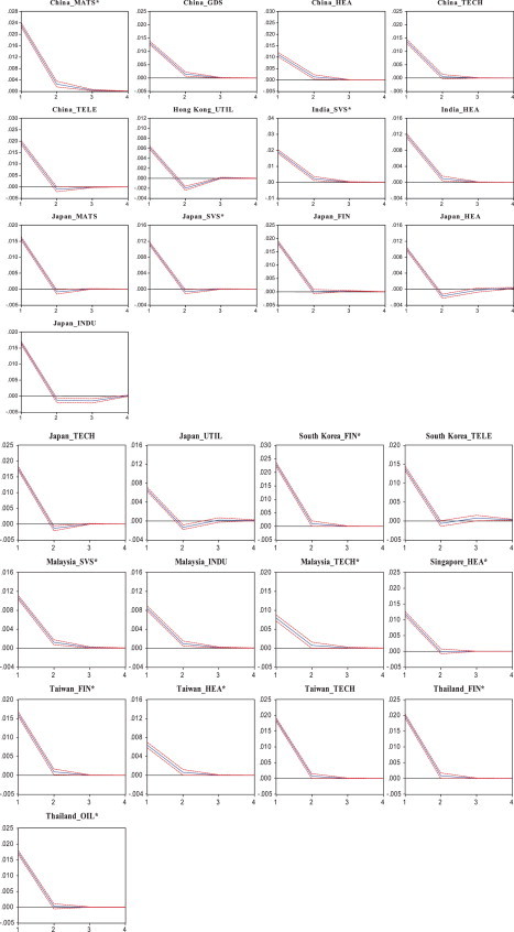
Generalized impulse response functions of market returns to an innovation in industry returns.
Note: ‘*’ denotes the 11 industry returns that lead stock market returns.
Among the 11 industry returns, 10 show that market returns respond positively to a shock from industry returns and are significant up to day 2, but the shock dies out in the third day. Except for Japan's SVS having a negative impact on market returns in day 2. Within 15 industry returns that have bi-directional relationships with market returns, 7 have salient negative relationships with market returns in day 2. The responses of the stock market from shocks INDU in Japan seems to have the most impact over time. The most dramatic negative effect is the response of the stock markets to UTIL in HK, UTIL in Japan, and to HEA in Japan. This result is consistent with the idea that investors prefer investments in some fall-resistant stocks – that is, when the market goes down, the specific-industrial stock returns increase.4
A one standard deviation shock to China's MATS (South Korea's FIN) raises the market returns by 0.23 or 0.24 points on the Chinese (South Korean) market returns in the first day. China's TELE and Thai's FIN follow thereafter. After 3 or 4 days, however, this impact quickly diminishes. Using monthly data, Hong et al. (2007) claim that stock markets react with a delay to information contained in industry returns.
This study agrees with Wang et al. (2003) who disclose significant industry effects on returns in current mainstream industries. Whereas Wang et al. (2003) show that computer software, electronics, semiconductors, and wireless and telecommunications equipment were the mainstream sectors during 1990–2001, we find that SVS and FIN are the current mainstream industries, and IT has diminished its importance in explaining market returns, which is consistent with Tessitore and Usmen (2005). We concur with Chen and De Bondt (2004) that styles perform variously over time.
3.5. The results of multiple structural breaks
Hendry (1997) and Clements and Hendry (1999) argue that many major failures of economic forecasts are due to the presence of structural breaks, which are represented by parameter instability. Therefore, to check whether the above findings hold when potential structural breaks and different time spans are considered, we first examine the VAR system under multiple structural changes. Table 4 presents the results of structural breaks, showing that stock markets in most countries do not have significant structural changes for the estimated period. A possible reason is that the daily data frequency used in this study is not easy to present structural changes due to the short interval. Even so, changes still exist for some industries in some countries, including MATS, SVS, and TELE in China, MATS in Hong Kong, SVS and FIN in Japan, FIN and OIL in South Korea, and INDU and TECH in Malaysia. Among the above ten industries presenting structure changes, only three are market leading industries (MAT in China, SVS in Japan, and TECH in Malaysia), signifying the relationships between the leading industry and market return are not affected by the structural break events.
Table 4.
Qu and Perron (2007) SupLR test for structural changes.
| Country | MATS | GDS | SVS | FIN | HEA | INDU | OIL | TECH | TELE | UTIL | |
|---|---|---|---|---|---|---|---|---|---|---|---|
| China | SupLR | 57.012 | 15.123 | 39.315 | 13.666 | 12.881 | 18.509 | 25.443 | 20.318 | 34.537 | 19.155 |
| Break | 2006/11/27 | 2006/12/26 | 2007/7/26 | ||||||||
| 2008/12/24 | 2008/12/25 | 2009/5/14 | |||||||||
| Hong Kong | SupLR | 56.282 | 5.432 | 18.324 | 20.751 | n.a. | 9.340 | 30.512 | 9.982 | 10.676 | 13.806 |
| Break | 2006/11/27 | ||||||||||
| 2008/12/18 | |||||||||||
| India | SupLR | 29.594 | n.a. | 22.099 | 27.970 | 24.266 | 29.881 | 12.922 | 19.114 | 10.106 | 26.725 |
| Break | |||||||||||
| Indonesia | SupLR | 19.685 | 17.206 | 15.435 | 11.592 | n.a. | n.a. | n.a. | n.d. | 16.083 | n.a. |
| Break | |||||||||||
| Japan | SupLR | 26.981 | 19.725 | 57.350 | 34.140 | 32.589 | 30.004 | 20.665 | 30.085 | 26.035 | 27.078 |
| Break | 2004/6/7 | 2004/7/14 | |||||||||
| 2007/7/26 | 2007/8/7 | ||||||||||
| South Korea | SupLR | 19.412 | 17.242 | 20.161 | 67.237 | 21.229 | 25.196 | 40.987 | 4.886 | 10.660 | 14.245 |
| Break | 2003/4/29 | 2004/8/2 | |||||||||
| 2008/8/29 | 2007/7/24 | ||||||||||
| Malaysia | SupLR | 15.967 | 16.099 | 12.955 | 24.839 | n.a. | 34.229 | 16.747 | 49.849 | 28.819 | 26.183 |
| Break | 2003/1/2 | 2003/7/10 | |||||||||
| 2006/11/23 | 2006/11/17 | ||||||||||
| Singapore | SupLR | 8.993 | n.a. | 25.214 | 5.274 | 20.402 | 22.639 | n.a. | 9.015 | 6.567 | n.d. |
| Break | |||||||||||
| Taiwan | SupLR | 8.572 | 1.287 | 9.707 | 1.969 | n.a. | 19.569 | n.a. | 5.562 | 18.706 | n.d. |
| Break | |||||||||||
| Thailand | SupLR | 17.971 | n.a. | 20.360 | 13.866 | n.a. | 20.549 | 10.929 | n.a. | 21.884 | 24.602 |
| Break |
Notes: m = 2 denotes two structural break points, which generate three regimes. The critical value for the 5% significance level is 33.454. SupLR denotes the SupLR test statistic. The null hypothesis is that there is no structural change. Break denotes the estimated date of structural changes. ‘n.a.’ denotes the test statistic cannot be computed, because the matrix is not positive definite. ‘n.d.’ denotes data are unavailable.
Most of the structure breaks that notably affect industries returns are: two coal mining disasters that happened on November 26, 2006 in China influence SVS in China, and MAT in China and Hong Kong;5 the global financial crisis (2008–2010) influences MAT, SVS, and TELE in China, MAT in Hong Kong, and FIN in South Korea; typhoons, floods, and mudslides (end-2003 to 2005) impact SVS and FIN in Japan;6 South Korea was the largest coalition partner after the U.S. and UK in the Iraq War and deployed troops in August 2004, which resulted in an influence on OIL in South Korea; SARS (2002–2003) outbreak influences FIN in South Korea, and INDU and TECH in Malaysia7 ; subprime crisis (July 2007) influences SVS and FIN in Japan, TELE and SVS in China, and OIL in South Korea; heavy rain showers hit Malaysia continuously every day for several weeks from November 2006, causing a series of flood to influence INDU and TECH in Malaysia.8
We further estimate the coefficients under different regimes for these industries by employing Qu and Perron's (2007) procedure, as shown in Table 5 .9 Distinct from other multiple structural breaks models, Qu and Perron's (2007) model can be applied to a system of equations, which allows us to consider the bi-directional relationships when examining the impact of industry returns on market returns. Based on the possible dates of structural changes, we divide the whole period into three sub-periods. The results show that in different sub-periods the stock returns of some industries in some countries have divergent effects, i.e., positive and negative, on the market returns respectively. On the other hand, Japan's SVS and Malaysia's INDU are negatively impacted by the structural changes, while Japan's FIN and Malaysia's TECH are positively impacted by the structural changes.
Table 5.
Estimated coefficients of structural changes – Market equation.
| Country | Industry | Regime 1 | Regime 2 | Regime 3 | |
|---|---|---|---|---|---|
| China | MATS | Period | 2001/01/01–2006/11/26 | 2006/11/27–2008/12/23 | 2008/12/24–2010/12/31 |
| Indt−1 | 0.103 | 0.102 | −0.024 | ||
| SVS | Period | 2001/01/01–2006/12/25 | 2006/12/26–2008/12/24 | 2008/12/25–2010/12/31 | |
| Indt−1 | 0.037 | −0.078 | −0.035 | ||
| TELE | Period | 2002/11/18–2007/7/25 | 2007/07/26–2009/05/13 | 2009/05/14–2010/12/31 | |
| Indt−1 | 0.004 | 0.186 | −0.145 | ||
| Hong Kong | MATS | Period | 2001/01/01–2006/11/26 | 2006/11/27–2008/12/17 | 2008/12/18–2010/12/31 |
| Indt−1 | 0.001 | −0.043 | −0.057 | ||
| Japan | SVS | Period | 2001/01/01–2004/06/06 | 2004/06/07–2007/07/25 | 2007/07/26–2010/12/31 |
| Indt−1 | −0.131 | −0.146 | −0.269 | ||
| FIN | Period | 2001/01/01–2004/07/13 | 2004/07/14–2007/08/06 | 2007/08/07–2010/12/31 | |
| Indt−1 | 0.078 | 0.077 | 0.075 | ||
| South Korea | FIN | Period | 2001/01/01–2003/04/28 | 2003/04/29–2008/08/28 | 2008/08/29–2010/12/31 |
| Indt−1 | −0.007 | 0.132 | −0.434 | ||
| OIL | Period | 2001/01/01–2004/08/01 | 2004/08/02–2007/07/23 | 2007/07/24–2010/12/31 | |
| Indt−1 | 0.000 | 0.015 | 0.049 | ||
| Malaysia | INDU | Period | 2001/01/01–2003/01/01 | 2003/01/02–2006/11/22 | 2006/11/23/2010/12/31 |
| Indt−1 | −0.056 | −0.032 | −0.017 | ||
| TECH | Period | 2001/01/01–2003/07/09 | 2003/07/10–2006/11/16 | 2006/11/17–2009/3/20 | |
| Indt−1 | 0.034 | 0.045 | 0.052 |
Notes: This table examines further the causality with multiple structural breaks, and thus only the significant industries of Table 4 are included in this test. Dependent variable is market return. Estimated break dates and coefficients are based on Qu and Perron (2007). Lagged market returns are omitted to save space.
China's MATS, SVS, and TELE are negatively influenced by structure breaks in regime 3, rather than regime 1. Whether the condition is due to the gradual openness of China's economy awaits further research investigation. The returns in regime 3 in these industries have a negative impact on the next-day market return. Interestingly, this sub-period starts in the latter half of 2008, or about the time of further deterioration from the global financial crisis.
The results have several implications for the investigation of stock market returns. The impact of industry returns on market returns varies in different periods, because of the emergence of unusual shocks or the phenomenon that some industries are influenced by business cycles. Hence, different conclusions may be achieved, suggesting that the occurrence of substantial shocks should be considered when exploring the effect of the return from certain industries on the market returns. The technique this article adopts of examining structural changes is a procedure that takes into account the property of data and endogenously determines multiple structural break points, thus providing objective results, which limit any discussion of prior works.
3.6. Market predictability across the business cycle
Jacobsen, Marshall, and Visaltanachoti (2011) find that Hong et al.’s (2007) findings are much stronger when accounting for sign-switching due to different sectors signaling good or bad news during contractions and expansions. To examine if the business cycle affects the prediction of the industry return for the market return, we take the business cycle into consideration. Following Jacobsen et al. (2011), we estimate the following regression:
| (10) |
where R t is the market return at time t, INDt−1 denotes the industry return at time t−1, and Expansiont−1 (Contractiont−1) is a dummy variable that equals 1 if the economy is expanding (contracting) and zero if it is contracting (expanding).
We examine the effect of the business cycle utilizing the data of Japan and Taiwan because only datasets from these two countries are readily available for expansion and contraction periods. As Table 6 shows, the business cycle matters more for the leading relationship between industries and the market in Japan than in Taiwan. For Japan the returns of six out of ten industries significantly impacts the market returns in the contraction period, and HEA and UTIL are associated with the market both in the expansion and contraction periods. In Taiwan, in contrast, the change in the business cycle in general does not make a difference in the relationship between industries and the market. Japan and Taiwan are characterized, respectively, as the developed versus developing economy, and therefore our results imply that the degree of economic development could be a factor influencing the effect of the business cycle on the industry-market relationship.10
Table 6.
Market predictability across the business cycle.
| MATS | GDS | SVS | FIN | HEA | INDU | OIL | TECH | TELE | UTIL | |
|---|---|---|---|---|---|---|---|---|---|---|
| Japan | ||||||||||
| β1 | −0.010 | −0.027 | −0.041 | 0.016 | −0.080** | −0.011 | −0.013 | 0.006 | −0.031 | −0.105*** |
| (0.025) | (0.026) | (0.031) | (0.022) | (0.035) | (0.024) | (0.022) | (0.020) | (0.022) | (0.035) | |
| β2 | −0.057 | −0.078* | −0.165*** | −0.078** | −0.152** | −0.063 | −0.048 | −0.052 | −0.090** | −0.199*** |
| (0.043) | (0.047) | (0.062) | (0.034) | (0.060) | (0.042) | (0.035) | (0.036) | (0.038) | (0.063) | |
| F-test | 0.885 | 0.894 | 3.224* | 5.437** | 1.068 | 1.112 | 0.732 | 2.013 | 1.834 | 1.700 |
| R2 | 0.0021 | 0.0039 | 0.0093 | 0.0055 | 0.0120 | 0.0027 | 0.0021 | 0.0024 | 0.0066 | 0.0170 |
| Taiwan | ||||||||||
| β1 | 0.018 | 0.005 | 0.014 | −0.002 | −0.027 | 0.030 | 0.005 | 0.047** | −0.002 | – |
| (0.030) | (0.024) | (0.027) | (0.029) | (0.028) | (0.026) | (0.022) | (0.023) | (0.039) | – | |
| β2 | 0.007 | 0.012 | 0.042 | 0.006 | −0.022 | 0.018 | −0.025 | 0.039 | 0.065 | – |
| (0.049) | (0.036) | (0.051) | (0.036) | (0.049) | (0.038) | (0.073) | (0.033) | (0.078) | – | |
| F-test | 0.0316 | 0.0291 | 0.245 | 0.0376 | 0.00583 | 0.0574 | 0.154 | 0.0470 | 0.574 | – |
| R2 | 0.0002 | 0.0001 | 0.0008 | 0.0000 | 0.0006 | 0.0008 | 0.0001 | 0.0027 | 0.0008 | |
Notes: Robust standard errors in parentheses. The regression model Rt = α + β1Expansiont−1INDt−1 + β2Contractiont−1INDt−1 + ɛt is run for each industry of each country, where Rt is the market return at time t, INDt−1 is the industry return at time t−1, and is a dummy variable that equals 1 if the economy is expanding (contracting) and zero if it is contracting (expanding) at time t−1. The F-test represents the Wald test determining whether β1 and β2 are statistically significantly different. *** Significance level of 1%; ** Significance level of 5%; * Significance level of 10%. “–” denotes data are not available. The business cycles of Japan and Taiwan are obtained from Cabinet Office of Japan (www.esri.cao.go.jp) and Council for Economic Planning and Development of Taiwan (www.cepd.gov.tw), respectively.
4. Robustness checks
4.1. Out-of-sample performance test
To evaluate whether the predicted return based on the industry leading model can provide a higher return than the historical average return, we perform an out-of-performance test. We follow Campbell and Thompson (2008), Welch and Goyal (2008), and Jacobsen et al. (2011) to compute an out-of-sample R 2 statistic and change in root mean squared predicted errors (ΔRMSE) to evaluate the performance of the predicted model adopted in this article.11
When performing an out-of-sample test, selecting an adequate estimation and evaluation periods is important. Welch and Goyal (2008) note that it is not clear how to choose adequate periods when estimating and then evaluating a regression model, but some criteria could be followed even though the choice is ad-hoc in the end. An important requirement is to have enough initial data to reliably estimate the regression model at the start of the evaluation period and the evaluation period needs to be long enough to be representative. As our data frequency is on a daily basis, we use 2010 as the out-of-sample forecast evaluation period and earlier data, i.e., 2001–2009, to estimate an initial regression. Furthermore, due to space limitation, we choose industries having a unidirectional causal effect on the market return to assess the performance of the predicted regression.12
Table 7 presents the results of the out-of-sample performance test. We examine if the predicted returns based on the industry leading regression is superior to the pure buy-and-hold returns (BHR). As the forecasted return based on the industry predicted regression (Column 3) shows, the predicted returns have a positive return, except SVS in Japan. Column 5 presents a positive in Japan, South Korea, Malaysia, Singapore, and Taiwan, suggesting that the predicted error of the market returns by the predicted regression is lower than by the historical average in these countries. The result signifies better predictability compared with BHD, even though the predicted strategy could not have a higher return than that of BHD. On average, our findings illustrate the usefulness of industry returns in predicting stock markets.
Table 7.
Out-of-sample performance test.
| Industry | BHR | Forecast | Difference | ΔRMSE | |
|---|---|---|---|---|---|
| China_MATS | −2.46 | 0.07 | *** | −0.43 | −0.05 |
| India_SVS | 5.40 | 0.06 | *** | −0.76 | −0.08 |
| Japan_SVS | 2.41 | -0.01 | *** | 0.79 | 0.07 |
| Korea_FIN | 2.79 | 0.06 | *** | 0.13 | 0.02 |
| Malaysia_SVS | 15.21 | 0.06 | *** | 1.71 | 0.12 |
| Singapore_HEA | 4.56 | 0.03 | *** | 0.05 | 4.35e-02 |
| Taiwan_FIN | −3.25 | 0.01 | *** | 0.34 | 0.03 |
| Taiwan_HEA | −3.25 | 0.01 | *** | 0.90 | 0.09 |
| Thailand_FIN | 17.71 | 0.07 | *** | −0.77 | −0.09 |
| Thailand_OIL | 17.71 | 0.07 | *** | −0.49 | −0.05 |
Notes: BHR denotes the buy-and-hold return. Forecast denotes the forecasted return based on the predicted industry regression. Difference is the mean difference between buy-and-hold return and forecasted return based on the industry leading regression. and ΔRMSE are the out-of-sample performance of forecasts relative to the historical average return introduced in Campbell and Thompson (2008), Welch and Goyal (2008), and Jacobsen et al. (2011). Industries are selected based on the unidirectional effect from the industry return to the market return as presented in Table 2. All figures relate to a one-year (2010) out-of-sample period and are in percentage terms. *** denote statistical significance at the 1% level.
4.2. Intermediate- and short-period tests
We further test the VAR system under short and intermediate periods to evaluate whether our empirical findings remain the same. The VAR model is re-estimated using the recent 3-year and 1-year periods, as summarized in Table 8 , with 10-year results listed as well for comparison purposes. The findings are not as salient as the aforementioned 10-year results, yet SVS, HEA, and FIN are still significant in the 3-year period for most of the countries. Four of the 7 results with unidirectional Granger causality from industry returns to market returns are HEA, indicating the importance of the HEA sector. Only UTIL for Japan is salient in the 1-year period, probably due to the short time span.
Table 8.
Robustness checks: Granger causality test of 26 industries for 3- and 1-year periods.
| Country | Periods | Industry returns Granger cause market returns |
|---|---|---|
| China | 10-year | MATS#, GDS, HEA, TECH, TELE |
| 3-year | GDS, HEA#, TECH, TELE | |
| 1-year | None | |
| Hong Kong | 10-year | UTIL |
| 3-year | None | |
| 1-year | None | |
| India | 10-year | SVS#, HEA |
| 3-year | HEA# | |
| 1-year | None | |
| Japan | 10-year | MATS, SVS#, FIN, HEA, INDU, TECH, UTIL |
| 3-year | MATS, SVS#, HEA#, INDU, TECH, UTIL | |
| 1-year | UTIL# | |
| South Korea | 10-year | FIN#, TELE |
| 3-year | FIN#, TELE | |
| 1-year | None | |
| Malaysia | 10-year | SVS#, INDU, TECH# |
| 3-year | SVS | |
| 1-year | None | |
| Singapore | 10-year | HEA# |
| 3-year | HEA# | |
| 1-year | None | |
| Taiwan | 10-year | FIN#, HEA#, TECH |
| 3-year | FIN# | |
| 1-year | None | |
| Thailand | 10-year | FIN#, OIL# |
| 3-year | None | |
| 1-year | None |
Notes: Tests use 1% and 5% significance levels respectively. Malaysia does not have 1-year data for the technology industry. Indonesian industries present no Granger causality with market returns. “#” indicates unidirectional Granger causality from industry returns to market returns; the remaining industries are bi-directional Granger causality with market returns. ‘None’ denotes the result does not show that industry returns are significant with Granger-caused market returns.
4.3. Alternative data frequency
We also perform a causality test using weekly and monthly data. To save space the monthly and weekly results are available from the authors on request. However, most of the aforementioned market-leading industries have insignificant predictive powers. The results are consistent with our GIRF results that all markets seem to settle back to their pre-shock level within four days. Thus, the daily data appears to be more informative than weekly or monthly ones. The predicted industry model fits only for high frequency data. The results correspond to the argument of Jacobsen, Marshall, and Visaltanachoti (2008) that if markets are near efficient, then predictability tests that rely on a full month of data to make a prediction may be less accurate than tests that use only the most recent few days of data.
5. Conclusion and implications
Different from conventional studies that mainly focus on the industry leading effect, we examine the industry leading, market leading, feedback, and neutrality hypotheses. It is well-known that Asia has an extremely bright future in the world economy, with economies that have the potential to develop quickly. This paper thus targets eastern and southern Asia and includes developed and emerging countries in order to gain more insight about stock markets in the area.
The results suggest that no matter when considering whether the model is estimated over a long or short time period or after looking at other factors, FIN and SVS returns have significant power in explaining the movements of market returns. Hong et al. (2007) also find that service and commercial real estate industry returns forecast the stock market. Generally, the market leading hypothesis is supported in most of OIL, GDS, and UTIL; the industry leading hypothesis in SVS and FIN; the feedback hypothesis in HEA and TECH; and the neutrality hypothesis in some of the other industries. Several factors determine the dominance of the alternative hypotheses, including GDP growth rate, exports, oil price, the exchange rate, the interest rate, and government support. These findings could shed some light for the government on establishing industry policies.
Different countries have different leading industries. FIN plays an important role in Taiwan, Thailand, and South Korea, while SVS plays an important role in India, Japan, and Malaysia. On the other hand, industry returns are led by market returns in some countries, including GDS in India, Indonesia, and Malaysia, OIL in Hong Kong, India, Japan, and Malaysia, and UTIL in China, Indonesia, Malaysia, and Thailand. The results could guide investors focusing on eastern and southern Asia when formulating their country- and industry-specific investment strategies.
Acknowledgement
We would like to thank Editor Hamid Beladi and the anonymous referees for their highly constructive comments.
Footnotes
Trading activity, measuring turnover by volume, denotes the number of shares traded for an industry on a particular day and is expressed the unit in thousands.
Please see Japan moves to improve efficiency of service sector, Japan External Trade Organization, October 2007. www.jetro.org.
Source: Taiwan Economic Journal.
We do not interpret insignificant parts of Granger causality in the GIRF section.
In 2006, according to the State Work Safety Supervision Administration, 4749 Chinese coal miners were killed in thousands of blasts, floods, and other accidents. Specifically, on November 26, 2006, explosions in two Chinese coal mines occurred the same day and together incurred the highest reported death toll for one day in China's notoriously dangerous mines in 2006.
In 2004, typhoons struck Japan in June, and frequent landfalls in July overwhelmed riverbanks and triggered mudslides at 370 locations. According to Japan's local governments, 24,000 houses were damaged due to the floods and mudslides.
Though South Korea and Malaysia did not see the most serious spread of SARS domestically, SARS did impact the industries in South Korea and Malaysia due to no other influential information or factors that may have stimulated a rise in national securities prices during the period.
According to CBC News, an estimated 400,000 people were displaced at the peak of the flooding and at least 118 people died with 155 people missing as of December 29, 2006. There were fears that flash flooding would occur in Malaysia. http://www.cbc.ca/news/world/story/2006/12/22/malaysia-flood.html.
We omit the results for the industry equation so that we can focus on the effect of industry returns on market returns (industry leading hypothesis). The results for the industry equations are available upon request.
As we cannot evaluate this possibility through examining all countries, we view the evidence as suggestive and leave it for the future research.
We do not delineate the computation here to save space and refer interested readers to these papers for details.
We exclude the technology industry in Malaysia as the data are unavailable after March 23, 2009.
Appendix A. Appendix
See Table A1 .
Table A1.
Summary statistics for daily returns.
| Country | Market | MATS | GDS | SVS | FIN | HEA | INDU | OIL | TECH | TELE | UTIL | |
|---|---|---|---|---|---|---|---|---|---|---|---|---|
| China | Mean | 0.0008 | 0.0009 | 0.0005 | 0.0008 | 0.0007 | 0.0003 | 0.0005 | 0.0009 | 0.0000 | 0.0004 | 0.0002 |
| S.D. | 0.0194 | 0.0260 | 0.0195 | 0.0215 | 0.0223 | 0.0246 | 0.0214 | 0.0233 | 0.0217 | 0.0250 | 0.0200 | |
| Skewness | −0.0987 | −0.1058 | 0.1389 | −0.2355 | 0.2912 | 0.6543 | 0.0620 | 0.0378 | −0.8799 | 0.2213 | −0.1999 | |
| Kurtosis | 10.8516 | 8.8589 | 9.0124 | 6.6986 | 9.2085 | 9.5464 | 10.7287 | 9.5616 | 18.6988 | 9.6928 | 9.6341 | |
| JB p-value | 0.0000 | 0.0000 | 0.0000 | 0.0000 | 0.0000 | 0.0000 | 0.0000 | 0.0000 | 0.0000 | 0.0000 | 0.0000 | |
| Hong Kong | Mean | 0.0003 | 0.0003 | 0.0006 | 0.0001 | 0.0003 | 0.0003 | 0.0002 | 0.0003 | 0.0002 | 0.0004 | 0.0003 |
| S.D. | 0.0146 | 0.0205 | 0.0174 | 0.0153 | 0.0160 | 0.0161 | 0.0159 | 0.0335 | 0.0242 | 0.0209 | 0.0104 | |
| Skewness | −0.1965 | −0.8507 | −0.1571 | −0.4364 | −0.1006 | −1.0285 | −0.2752 | −13.0166 | −0.0448 | 0.1291 | −0.3513 | |
| Kurtosis | 9.0874 | 15.0688 | 6.7068 | 11.5041 | 7.8001 | 15.2041 | 8.9056 | 474.06 | 6.2592 | 6.4617 | 32.7028 | |
| JB p-value | 0.0000 | 0.0000 | 0.0000 | 0.0000 | 0.0000 | 0.0000 | 0.0000 | 0.0000 | 0.0000 | 0.0000 | 0.00002 | |
| India | Mean | 0.0006 | 0.0009 | 0.0009 | 0.0002 | 0.0009 | 0.0005 | 0.0009 | 0.0003 | 0.0004 | 0.0003 | 0.0008 |
| S.D. | 0.0183 | 0.0239 | 0.0163 | 0.0321 | 0.0226 | 0.0151 | 0.0211 | 0.0233 | 0.0253 | 0.0249 | 0.0238 | |
| Skewness | −0.2300 | −0.2026 | 0.7327 | −0.0996 | −0.0945 | −0.2097 | −0.0314 | −0.3192 | −0.4671 | 0.1575 | −0.5783 | |
| Kurtosis | 11.6469 | 8.5550 | 18.3690 | 8.3877 | 11.2131 | 10.4511 | 9.5653 | 10.6447 | 11.0616 | 9.6803 | 13.3603 | |
| JB p-value | 0.0000 | 0.0000 | 0.0000 | 0.0000 | 0.0000 | 0.0000 | 0.0000 | 0.0000 | 0.0000 | 0.0000 | 0.0000 | |
| Indonesia | Mean | 0.0009 | 0.0008 | 0.0013 | −0.0002 | 0.0009 | 0.0002 | 0.0011 | 0.0011 | – | 0.0007 | 0.0011 |
| S.D. | 0.0213 | 0.0317 | 0.0294 | 0.0244 | 0.0261 | 0.0145 | 0.0281 | 0.0802 | – | 0.0244 | 0.0272 | |
| Skewness | −0.4861 | −0.4568 | −0.0351 | −0.3922 | 0.1805 | −0.3566 | 17.3369 | 28.3682 | – | −0.2333 | 0.0378 | |
| Kurtosis | 10.8269 | 12.7371 | 8.7682 | 6.8762 | 10.4723 | 20.8364 | 627.91 | 949.0343 | – | 9.7356 | 16.9098 | |
| JB p-value | 0.0000 | 0.0000 | 0.0000 | 0.0000 | 0.0000 | 0.0000 | 0.0000 | 0.0000 | – | 0.0000 | 0.0000 | |
| Japan | Mean | 0.0000 | 0.0001 | 0.0001 | 0.0000 | −0.0002 | 0.0000 | 0.0000 | 0.0002 | −0.0002 | −0.0001 | 0.0001 |
| S.D. | 0.0150 | 0.0174 | 0.0160 | 0.0132 | 0.0205 | 0.0132 | 0.0177 | 0.0200 | 0.0200 | 0.0183 | 0.0123 | |
| Skewness | −0.1179 | −0.1318 | −0.0555 | −0.1008 | 0.0612 | −0.3671 | −0.1126 | −0.1756 | 0.0245 | −0.1135 | −0.0975 | |
| Kurtosis | 6.8166 | 7.6325 | 6.8792 | 5.5877 | 6.1941 | 8.9462 | 6.8347 | 5.5882 | 5.6426 | 6.1803 | 6.4224 | |
| JB p-value | 0.0000 | 0.0000 | 0.0000 | 0.0000 | 0.0000 | 0.0000 | 0.0000 | 0.0000 | 0.0000 | 0.0000 | 0.0000 |
| Country | Market | MATS | GDS | SVS | FIN | HEA | INDU | OIL | TECH | TELE | UTIL | |
|---|---|---|---|---|---|---|---|---|---|---|---|---|
| South Korea | Mean | 0.0006 | 0.0010 | 0.0008 | 0.0005 | 0.0005 | 0.0004 | 0.0010 | 0.0009 | 0.0012 | −0.0000 | 0.0001 |
| S.D. | 0.0214 | 0.0251 | 0.0238 | 0.0216 | 0.0257 | 0.0211 | 0.0262 | 0.0282 | 0.0809 | 0.0186 | 0.0225 | |
| Skewness | −0.1860 | −0.2768 | −0.1261 | 1.3305 | −0.1296 | −0.1538 | −0.3649 | 0.3282 | 36.7139 | 0.2599 | 0.4039 | |
| Kurtosis | 16.5666 | 14.9092 | 11.4311 | 33.6666 | 11.8251 | 8.5535 | 13.5975 | 18.4333 | 1680.8780 | 8.8986 | 15.6033 | |
| JB p-value | 0.0000 | 0.0000 | 0.0000 | 0.0000 | 0.0000 | 0.0000 | 0.0000 | 0.0000 | 0.0000 | 0.0000 | 0.0000 | |
| Malaysia | Mean | 0.0004 | 0.0006 | 0.0006 | 0.0006 | 0.0005 | 0.0003 | 0.0002 | 0.0004 | −0.0005 | 0.0003 | 0.0002 |
| S.D. | 0.0103 | 0.0300 | 0.0147 | 0.0135 | 0.0123 | 0.0056 | 0.0137 | 0.0138 | 0.0194 | 0.0138 | 0.0112 | |
| Skewness | −0.6806 | 29.6508 | −0.0152 | 0.1599 | −0.3353 | −0.2863 | −6.8307 | −1.3765 | 0.5135 | −0.0975 | −1.1852 | |
| Kurtosis | 11.9211 | 1136.07 | 12.1339 | 6.3921 | 8.3751 | 12.0967 | 177.4654 | 32.7731 | 11.2668 | 8.4881 | 18.7592 | |
| JB p-value | 0.0000 | 0.0000 | 0.0000 | 0.0000 | 0.0000 | 0.0000 | 0.0000 | 0.0000 | 0.0000 | 0.0000 | 0.0000 | |
| Singapore | Mean | 0.0003 | 0.0008 | 0.0010 | 0.0003 | 0.0003 | 0.0008 | 0.0005 | 0.0006 | −0.0005 | 0.0002 | – |
| S.D. | 0.0141 | 0.0226 | 0.0244 | 0.0143 | 0.0159 | 0.0198 | 0.0161 | 0.3423 | 0.0254 | 0.0167 | – | |
| Skewness | −0.2397 | −0.0844 | 3.7000 | −0.1246 | −0.0393 | −0.0557 | −0.1848 | 5.3343 | 0.2009 | −0.4856 | – | |
| Kurtosis | 7.8024 | 13.2907 | 83.3013 | 6.4272 | 7.4077 | 9.0246 | 9.0750 | 895.7147 | 14.9331 | 9.6462 | – | |
| JB p-value | 0.0000 | 0.0000 | 0.0000 | 0.0000 | 0.0000 | 0.0000 | 0.0000 | 0.0000 | 0.0000 | 0.0000 | – | |
| Taiwan | Mean | 0.0002 | 0.0005 | 0.0003 | 0.0003 | 0.0002 | −0.0000 | 0.0003 | 0.0000 | 0.0001 | 0.0001 | – |
| S.D. | 0.0167 | 0.0167 | 0.0206 | 0.0170 | 0.0192 | 0.0151 | 0.0190 | 0.0139 | 0.0195 | 0.0118 | – | |
| Skewness | −0.0680 | 0.0661 | −0.0942 | −2.1792 | −0.0338 | 0.0124 | −0.0817 | −6.4443 | −0.0533 | −0.3018 | – | |
| Kurtosis | 5.0665 | 5.5219 | 5.1904 | 45.1032 | 5.1953 | 8.7391 | 4.5069 | 176.1651 | 4.7346 | 9.0003 | – | |
| JB p-value | 0.0000 | 0.0000 | 0.0000 | 0.0000 | 0.0000 | 0.0000 | 0.0000 | 0.0000 | 0.0000 | 0.0000 | – | |
| Thailand | Mean | 0.0007 | 0.0010 | 0.0005 | 0.0005 | 0.0006 | 0.0003 | 0.0005 | 0.0010 | 0.0003 | 0.0003 | 0.0006 |
| S.D. | 0.0174 | 0.0217 | 0.0148 | 0.0162 | 0.0221 | 0.0102 | 0.0231 | 0.0209 | 0.0147 | 0.0221 | 0.0176 | |
| Skewness | −0.6503 | −0.5541 | 1.4422 | 0.0071 | −0.1878 | 0.0504 | 0.2234 | −0.2760 | 0.0844 | −0.5356 | −0.0495 | |
| Kurtosis | 12.3326 | 10.7819 | 50.4401 | 9.0749 | 9.5032 | 12.0061 | 14.6825 | 9.6733 | 10.7085 | 12.5790 | 20.3667 | |
| JB p-value | 0.0000 | 0.0000 | 0.0000 | 0.0000 | 0.0000 | 0.0000 | 0.0000 | 0.0000 | 0.0000 | 0.0000 | 0.0000 | |
| Total average returns | 0.00048 | 0.00069 | 0.00066 | 0.00031 | 0.00047 | 0.00031 | 0.00052 | 0.00057 | 0.000111 | 0.00026 | 0.000425 | |
| Total average S.D. | 0.01685 | 0.02356 | 0.01969 | 0.01891 | 0.02027 | 0.01553 | 0.02023 | 0.05994 | 0.0279 | 0.01965 | 0.018125 |
Notes: Both Singapore and Taiwan data lack UTIL industry, while Indonesia data lack TECH. ‘–’ denotes data are unavailable. The cells which are shaded signify the largest statistics.
References
- Ariffin N., Figueiredo P.N. Internationalisation of innovative capabilities: Counter-evidence from the electronics industry in Malaysia and Brazil. Oxford Development Studies. 2004;32:559–583. [Google Scholar]
- Arnold W. Singapore goes for biotechnology. New York Times. 2003 August 26, W1. [Google Scholar]
- Bai J., Perron P. Computation and analysis of multiple structural change models. Journal of Applied Econometrics. 2003;18:1–22. [Google Scholar]
- Bekaert G., Harvey C.R., Lundblad C.T. Equity market liberalization in emerging markets. Journal of Financial Research. 2003;26:275–299. [Google Scholar]
- Bekaert G., Urias M. Diversification, integration and emerging market closed end funds. Journal of Finance. 1996;51:835–868. [Google Scholar]
- Bird K., Hill H., Cuthbertson S. Making trade policy in a new democracy after a deep crisis: Indonesia. The World Economy. 2008;31(7):947–968. [Google Scholar]
- Campbell J.Y., Thompson S.B. Predicting excess returns out of sample: Can anything beat the historical average. Review of Financial Studies. 2008;21:1509–1531. [Google Scholar]
- Chang C.L., McAleer M., Tansuchat R. Conditional correlations and volatility spillovers between crude oil and stock index returns. North American Journal of Economics and Finance. 2013;25:116–138. [Google Scholar]
- Chang P.L., Hsu C.W. The development strategies for Taiwan's semiconductor industry. IEEE Transactions on Engineering Management. 1998;45:349–356. [Google Scholar]
- Chen C., Martin X., Wang X. Insider trading, litigation concerns, an auditor going–concern opinions. Accounting Review. 2012;88(2):365–393. [Google Scholar]
- Chen G.M., Firth M., Rui O.M. Stock market linkages: Evidence from Latin American. Journal Banking and Finance. 2002;26:1113–1141. [Google Scholar]
- Chen H.L., De Bondt W. Style momentum within the S&P-500 index. Journal of Empirical Finance. 2004;11:483–507. [Google Scholar]
- Clements M.P., Hendry D.F. MIT Press; Cambridge, MA: 1999. Forecasting non-stationary economic time series. [Google Scholar]
- Dodgson M., Mathews J., Kastelle T., Hu M.C. The evolving nature of Taiwan's national innovation system: The case of biotechnology innovation networks. Research Policy. 2008;37:430–445. [Google Scholar]
- Dossani R., Kenny M. The next wave of globalization: Relocating service provision to India. World Development. 2007;35:772–791. [Google Scholar]
- Eichengreen B., Gupta P. India Council for Research on International Economic Relations; 2010. The service sector as India's road to economic growth? Working paper no. 249. [Google Scholar]
- Fukao K., Hamagata S., Miyagawa T., Tonogi K. Intangible investment in Japan: Measurement and contribution to economic growth. Review of Income and Wealth. 2009;55:717–736. [Google Scholar]
- Gelain P. The external finance premium in the Euro area: A dynamic stochastic general equilibrium analysis. North American Journal of Economics and Finance. 2010;21:49–71. [Google Scholar]
- Geske R., Roll R. The fiscal and monetary linkage between stock returns and inflation. Journal of Finance. 1983;38:1–33. [Google Scholar]
- Gin B.S. Singapore: A global biomedical sciences hub. Drug Discovery Today. 2005;10(1):1134–1137. doi: 10.1016/S1359-6446(05)03475-6. [DOI] [PubMed] [Google Scholar]
- Grace C. 2004. The effect of changing intellectual property on pharmaceutical industry prospects in India and China: Considerations for access to medicines.http://www.dfid.gov.uk/pubs/files/indiachinadomporduce.pdf [Google Scholar]
- Granger C.W.J. Investigating causal relations by econometric models and cross-spectral methods. Econometrica. 1969;37(3):424–438. [Google Scholar]
- Griffin J.M., Karolyi G.A. Another look at the role of the industrial structure of markets for international diversification strategies. Journal of Financial Economics. 1998;50:351–373. [Google Scholar]
- Hawkins D.M. Point estimation of the parameters of piecewise regression models. Applied Statistics. 1976;25:51–57. [Google Scholar]
- Hendry A. Trend, cycles and autoregressions. Economic Journal. 1997;107:192–201. [Google Scholar]
- Hong H., Torous W., Valkanov R. Do industries lead stock markets? Journal of Financial Economics. 2007;83:367–396. [Google Scholar]
- Hsu Y.G., Shyu J.Z., Tzeng G.H. Policy tools on the formation of new biotechnology firms in Taiwan. Technovation. 2005;25:281–292. [Google Scholar]
- Huang C.J., Fu T.T. Uncertainty and total factor productivity in the Taiwanese banking industry. Applied Financial Economics. 2009;19:753–766. [Google Scholar]
- Ito H. Financial development and financial liberalization in Asia: Thresholds, institutions and the sequence of liberalization. North American Journal of Economics and Finance. 2006;17:303–327. [Google Scholar]
- Jacobsen B., Marshall B., Visaltanachoti N. Massey University; 2008. Return predictability revisited. Working paper. [Google Scholar]
- Jacobsen B., Marshall B.R., Visaltanachoti N. 23rd Australasian Finance and Banking Conference 2010 Paper. 2011. Sign-switching return predictability. [Google Scholar]
- Johnson S., Mitton T. Cronyism and capital controls: Evidence from Malaysia. Journal of Financial Economics. 2003;67:351–382. [Google Scholar]
- Johnston M. 2010. Global X launches China materials ETF. ETF Database. http://seekingalpha.com/article/182549-global-x-launches-china-materials-etf. [Google Scholar]
- Jongwanich J., Park D. Inflation in developing Asia. Journal of Asian Economics. 2009;20:507–518. [Google Scholar]
- Jorgenson D.W., Nomura K. The industry origins of Japanese economic growth. Journal of the Japanese and International Economies. 2005;19:482–542. [Google Scholar]
- Kang S.H., Yoon S.M. Asymmetric long memory feature in the volatility of Asian stock markets. Asia-Pacific Journal of Financial Studies. 2006;35(5):175–198. [Google Scholar]
- Kaul G. Stock returns and inflation: The role of the monetary sector. Journal of Financial Economics. 1987;18:253–276. [Google Scholar]
- Keim D. Size related anomalies and stock return seasonality: Further empirical evidence. Journal of Financial Economics. 1983;12:13–32. [Google Scholar]
- Kim J.W., Leatham D.J., Bessler D.A. REIT's dynamics under structural change with unknown break points. Journal of Housing Economics. 2007;16:37–58. [Google Scholar]
- Lam P.L., Chan Y.C. Privatizing water supply in Hong Kong. Utilities Policy. 1998;7:95–105. [Google Scholar]
- Lee C.C. Insurance and real output: The key role of banking activities. Macroeconomic Dynamics. 2013;17:235–260. [Google Scholar]
- Lee C.C., Chang C.P. Structural breaks, energy consumption, and economic growth revisited: Evidence from Taiwan. Energy Economics. 2005;27:857–872. [Google Scholar]
- Lee C.C., Chen M.P., Hsieh K.M. Industry herding and market states: Evidence from the Chinese stock market. Quantitative Finance. 2013;13(7):1091–1113. [Google Scholar]
- Lee C.C., Huang W.L., Yin C.H. The dynamic interactions among the stock, bond and insurance markets. North American Journal of Economics and Finance. 2013;26:28–52. [Google Scholar]
- Lin C.H., Shiu C.Y. Foreign ownership in the Taiwan stock market—an empirical analysis. Journal of Multinational Financial Management. 2003;13:19–41. [Google Scholar]
- Luk S. A further assessment of the Hong Kong government's proposed post-2008 regulatory regime for local electricity utilities. Energy Policy. 2007;35:1423–1425. [Google Scholar]
- Pesaran M.H., Shin Y. Generalized impulse response analysis in linear multivariate models. Economics Letters. 1998;58:17–29. [Google Scholar]
- MaPherson E.M. Chapter 16 – Early uses of legislation to build industry. Plant Location Selection Techniques. 1995:150–161. [Google Scholar]
- Ministry of International Trade and Industry . 2007. Trade and transport facilitation: The Malaysian experience and milestone.www.unescap.org/tid/products/egmtf_s3Damiri.pdf [Google Scholar]
- Okuda H., Rungsomboon S. Hitotsubashi University; 2004. Comparative cost study of foreign and Thai domestic banks 1990-2002: Estimating cost functions of the Thai banking industry. CEI Working Paper series No. 2004-19. [Google Scholar]
- Park K.H., Weber W.L. A note on efficiency and productivity growth in the Korean banking industry, 1992-2002. Journal of Banking and Finance. 2006;30:2371–2386. [Google Scholar]
- Patro D. 2002. Stock market liberalization and emerging market country fund premiums, unpublished Rutgers University working paper. [Google Scholar]
- Qu Z., Perron P. Estimating and testing structural changes in multivariate regressions. Econometrica. 2007;75(2):459–502. [Google Scholar]
- Raju S.S., Melo A. Money, real output, and deficit effects of coffee booms in Colombia. Journal of Policy Modeling. 2003;25:963–983. [Google Scholar]
- Ritter J.R. Economic growth and equity returns. Pacific-Basin Finance Journal. 2005;13:489–503. [Google Scholar]
- Roll R. Industrial structure and the comparative behavior of international stock market indices. Journal of Finance. 1992;42:3–41. [Google Scholar]
- Serra A.P. Country and industry factors in returns—evidence from emerging markets’ stocks. Emerging Markets Review. 2000;1:127–151. [Google Scholar]
- Shahi G. BioEnterprise Asia; Singapore: 2004. Biobusiness in Asia. [Google Scholar]
- Tcha D.W., Park J.S., Chang S.G., Song K.H. Korean telecommunication industry in transition. Telecommunication Systems. 2000;14:3–12. [Google Scholar]
- Tessitore A., Usmen N. Relative importance of industry and country factors in security returns. Global Finance Journal. 2005;16:16–25. [Google Scholar]
- Torres A., Vela O. Trade integration and synchronization between the business cycles of Mexico and the United States. North American Journal of Economics and Finance. 2003;14:319–342. [Google Scholar]
- Tsuji C. Do industries contain predictive information for the Fama-French factors? Quantitative Finance. 2012;12(6):969–991. [Google Scholar]
- Vassalou M. News related to future GDP growth as a risk factor in equity returns. Journal of Financial Economics. 2003;68:47–73. [Google Scholar]
- Wang C.J., Lee C.H., Huang B.N. An analysis of industry and country effects in global stock returns: Evidence from Asian countries and the US. Quarterly Review of Economics and Finance. 2003;43:560–577. [Google Scholar]
- Wang Q. Price clustering of IPOs in the secondary market. Applied Economics Letters. 2010;17(13):1285–1292. [Google Scholar]
- Wang S., Mayes D.G. Monetary policy announcements and stock returns: An international comparison. North American Journal of Economics and Finance. 2012;23:145–164. [Google Scholar]
- Welch I., Goyal A. A comprehensive look at the empirical performance of equity premium prediction. Review of Financial Studies. 2008;21:1455–1508. [Google Scholar]
- Woo C.K., Horowitz I., Tishler A. A critical assessment of the Hong Kong Government's proposed post-2008 regulatory regime for local electricity utilities. Energy Policy. 2006;34:1451–1456. [Google Scholar]
- Wu J.C. The mineral industry of Thailand: U.S. Geological Survey Minerals Yearbook. http://minerals.usgs.gov/minerals/pubs/country/2004/thmyb04.pdf
- Yang L., Tapon F., Sun Y. International correlations across stock markets and industries: Trends and patterns 1988–2002. Applied Financial Economics. 2006;16:1171–1183. [Google Scholar]
- Yu F.L.T. Taiwan's entrepreneurs and international coordination: Evolution of global production network in electronics and IT industries. Global Economic Review. 2009;38(1):49–62. [Google Scholar]