BrainAGE and regional volumetric analysis of a Buddhist monk: a longitudinal MRI case study

Abstract

Yongey Mingyur Rinpoche (YMR) is a Tibetan Buddhist monk, and renowned meditation practitioner and teacher. YMR, now in his forties, has spent an extraordinary number of hours of his life meditating. Given recent interest in the potential effects of meditation on brain health, we sought to examine the aging profile of this expert meditato’s brain in comparison to that of the general population. To do this, we made use of the BrainAGE machine learning classifier, which computes an individual’s “brain age”, based on levels of gray matter volume throughout the brain, and allows assessment of the difference between an individual’s brain age and calendar age. We also conducted univariate analyses of gray matter volume changes over time, in specific regions previously implicated in meditation-related structural brain changes. We acquired T₁-weighted MRI scans of YMR’s brain at four time points between 2002 and 2016. MRI scans from 105 comparison subjects in the general population were also acquired. The primary findings from our analysis are as follows. First, YMR’s brain age advanced at a slower rate than his calendar age, and his brain aging rate was slower than that of the general population. Qualitatively, YMR’s brain indicated early maturation but delayed aging. Second, YMR’s brain, based on his latest scan in 2016, at his calendar age of 41 years, resembled that of an average 33-year-old’s from the compared general population. Third, we did not find statistically significant differences between YMR and the general population, in gross volumetric changes over time in the specific regions, suggesting that the detected brain aging differences may arise from more coordinated changes spread throughout the gray matter. Overall, these findings prompt more systematic longitudinal evaluation of the relationship between extensive meditation practice and aging of the brain.

1. INTRODUCTION

The last decade has seen a surge of interest in the effects of meditation practice on biological aging. While still a nascent literature, studies to date have provided evidence that meditation training may slow the attrition of telomeres (the protective caps on chromosomes) (Alda et al., 2016; Epel, Daubenmier, Moskowitz, Folkman, & Black-burn, 2009; Le Nguyen et al., 2019; Schutte & Malouff, 2014) and the loss of the brain’s gray matter (Lazar et al., 2005; Luders, Cherbuin, & Gaser, 2016; Luders, Cherbuin, & Kurth, 2015; Pagnoni & Cekic, 2007) that naturally occur with aging. Hypothesized mediators of mindfulness meditation’s effect on aging include its role in stress reduction and positive mood promotion, though much remains unknown about the mechanisms by which mindfulness meditation may achieve these effects (Kurth, Cherbuin, & Luders, 2017). To date, studies examining the relationship between mindfulness meditation and aging-related gray matter loss have primarily been cross-sectional. For instance, studies have observed that the negative correlation between age and gray matter volume in long-term meditators is lesser in magnitude than in non-meditators in the general population (Luders et al., 2015), and that the brain-age of long-term meditators is less than that of non-meditators of the same calendar-age (Luders et al., 2016). Here, we present a case study of a unique longitudinal data-set - consisting of four measurements spanning over a decade - of Tibetan Buddhist meditation master Yongey Mingyur Rinpoche (YMR).

The following sections present essential details of YMR’s background to highlight his substantial meditation training and experience throughout his life, which makes MRI data of his brain uniquely valuable.

Familial origins.

YMR was born in 1975¹, in Nubri, a small Himalayan village near the border of Nepal and Tibet. He is the son of the renowned meditation master, Tulku Urgyen Rinpoche and Sonam Chödrön. YMR was drawn to a life of contemplation from an early age, and would often wander away to meditate in solitude.

Childhood.

At the age of nine YMR left Nubri to study meditation with his father at Nagi Gompa, a small hermitage on the outskirts of Kathmandu valley. For nearly three years, Tulku Urgyen guided him through the Buddhist practices of Mahamudra and Dzogchen, teachings that are among the most advanced practices of Tibetan Buddhism. When he turned eleven YMR was requested to reside at Sherab Ling Monastery in Northern India, the seat of Tai Situ Rinpoche and one of the most important monasteries in the Kagyu lineage. While there, he studied the rituals of the Karma Kagyu lineage with the retreat master of the monastery, Lama Tsultrim. Within a year, at the age of twelve, he was formally enthroned as the seventh incarnation of Yongey Mingyur Rinpoche by Tai Situ Rinpoche.

Adolescence.

When YMR turned thirteen, he entered a traditional three year retreat under the guidance of Saljey Rinpoche. When YMR completed his three-year retreat, he was appointed as the Sherab Ling Monasterys next retreat master, in which he was responsible for guiding senior monks and nuns through the intricacies of Buddhist meditation practice in the next three-year retreat, a role that he continues to play to this day. The seventeen-year old YMR was one of the youngest lamas to ever hold this position.

Young adulthood.

When he was nineteen, he enrolled at Dzongsar Monastic College, where he studied the primary topics of the Buddhist academic tradition, including Middle Way philosophy and Buddhist logic. When he was twenty years old, he was asked to oversee the activities of Sherab Ling Monastery. In his new role, he helped establish a new monastic college at the monastery, where he worked as an assistant professor while also carrying out his duties as retreat master for a third three year retreat. Throughout this period, which lasted until he was twenty-five, YMR often stayed in retreat for periods of one to three months while continuing to oversee the activities of Sherab Ling Monastery. When he was twenty-three years old, he received full monastic ordination from Tai Situ Rinpoche.

Adulthood.

In the years that followed, YMR continued to study the Buddhist tradition and perform daily meditative practice and periodic solitary retreats. He has also been active as a meditation teacher, and has led meditation retreats around the world for more than twenty years. To this day, YMR continues his studies and meditation. In early June, 2011, YMR walked out of his monastery in Bodhgaya, India and began a wandering retreat through the Himalayas and the plains of India that lasted four and a half years.

Involvement in science.

In addition to his extensive background in meditation and Buddhist philosophy, YMR has held a lifelong interest in psychology and neuroscience. At an early age, he began a series of informal discussions with neuroscientist Francisco Varela, who came to Nepal to learn meditation from his father, Tulku Urgyen Rinpoche. In 2002, YMR and a handful of other long-term meditators were invited to the Waisman Laboratory for Brain Imaging and Behavior, at the University of Wisconsin-Madison, at the request of His Holiness the Dalai Lama to examine the effects of meditation practices on the brain. YMR continues his involvement with this research as an advisor and as a participant in the ongoing studies of the neural and physiological effects of meditation.

2. METHODS

Subjects.

YMR was scanned in the years 2002, 2005, 2007, and 2016, when his calendar age was 27, 30, 32 and 41 years, respectively. In addition, 105 adult participants from the general population were scanned between 2010 and 2011 for one (n = 105), two (n = 105), or three (n = 30) time points. The average calendar age of the general population cohort at the time of their first scan was 48.66 (±10.90) years. Their age range is from 25.97 to 66.42 years. This cohort consisted of 65 women and 40 men. Participants in the general population cohort were recruited for a study on health and well-being through advertisements in Madison, WI, area newspapers, e-mails, and through postings and discussions with meditation teachers and groups. Exclusion criteria included use of psychotropic or steroid drugs, night-shift work, diabetes, peripheral vascular disease or other diseases affecting circulation, needle phobia, pregnancy, current smoking habit, alcohol or drug dependency, current or previous use of medication for anxiety, depression, or other psychological issues, psychiatric diagnosis in the past year, any history of bipolar or schizophrenic disorders, brain damage or seizures, significant previous experience with meditation or other mindbody techniques, and remarkable exercise habits (engagement in moderate sport or recreational activities for more than 5 hours per week or engagement in vigorous sport or recreational activities for more than 4 hours per week). The distribution of ages, and the age differences between consecutive MRI visits are shown in Fig. 1. Between time point 1 and time point 2, n = 34 subjects completed an 8-week mindfulness-based stress reduction (MBSR) course, and n = 36 subjects completed a health enhancement program (HEP). n = 35 subjects did not partake in either program.

Figure 1.: Calendar age distributions.

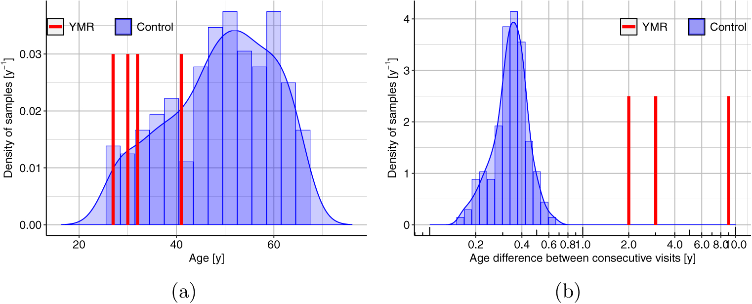
(a) Calendar ages. (b) Calendar age intervals between consecutive MRI visits. Since the longitudinal age differences for the controls were all less than one year, and those for YMR were all two or more years, the control data were treated cross-sectionally. With less than a year age difference for controls, the longitudinal change curves would not capture the rates of changes that would be needed to compare against data on YMR.

In a typical statistical analysis one would need to have samples from two groups matched on the factors such as age or gender. But in this case, rather than estimating the statistical significance of the coefficients of independent variables in a (say linear) model, the goal is to estimate the predictive power of the model jointly with all the coefficients. Furthermore, the age is actually the outcome variable in this case, and it would be important for the model to see a wide dynamic range of the mapping between brain image voxels and the calendar ages. Especially because the changes in a typical brain are not drastic on a T₁-weighted MRI scan for the age window of 27 to 41 years. In fact, the larger the number of samples and the wider the age range on which the model is trained the more accurate and reliable the prediction power of the model would be. For example, the model trained in the paper (Cole et al., 2018) cited within (Beheshti, Nugent, Potvin, & Duchesne, 2019), the model was trained on n = 3377 scans from seven different publicly available studies with an age range of 18–90 years.

Since the longitudinal age differences between consecutive MRI scans for the controls were all less than one year, and those for YMR were all two or more years, the control data were treated cross-sectionally, since their individual longitudinal changes would be on a significantly different time scale compared to those of YMR. If, for example, we had access to longitudinal data for controls that spanned similar age ranges to that of YMR’s sampling, we could have trained machine learning models similar to those used in time series prediction or those used in the natural language processing (e.g. translation, summarization, email response prediction) where both the sample features and the outcomes have temporal dependency and ordering information (such as grammatical ordering of words in a sentence) incorporated. In fact, even for YMR, the longitudinal nature of the data was not explicitly used in the relevance vector machine training.

Imaging.

Brain imaging took place at Waisman Laboratory for Brain Imaging and Behavior. Images for the general population cohort were acquired on a GE 750 3.0 T MRI scanner device with an eight-channel head coil. Anatomical scans consisted of a high-resolution 3D T₁-weighted inversion recovery fast gradient echo image (inversion time = 450 ms, 256 × 256 in-plane resolution, 256 mm FOV, 124 × 1.0 mm axial slices). The images for YMR for the first three time points (2002, 2005 and 2007) were acquired on GE 3.0 T Signa MRI scanner. Scanner was upgraded to GE 750 3.0 T in 2009, and the fourth time point (2016) data were acquired on the upgraded scanner. Representative slices, in the three orthogonal directions, are shown for all the four time points in Fig. 2. He was scanned on three consecutive days in 2002, on two consecutive days in 2005, and once in 2007 and 2016. For the first two time points, the processed data were averaged over the multiple days.

Figure 2.: Representative slices of YMR’s brain from the different years he volunteered.

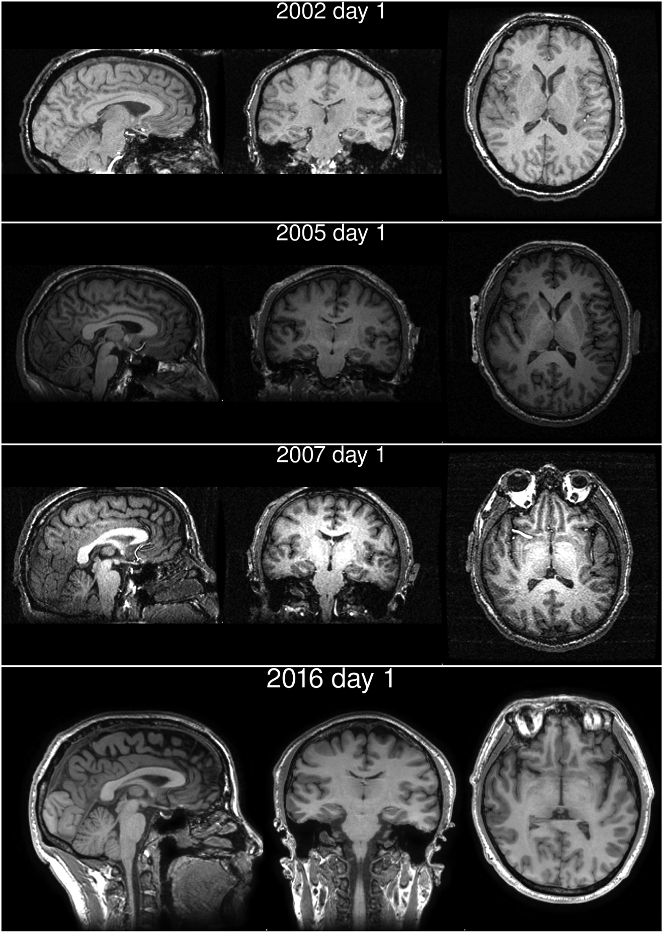
Image intensities are shown with the same window levels across the years. Changes in the bias levels of those intensities were accounted for by the processing pipeline (Fig. 3) and the BrainAGE estimation framework. (Franke et al., 2013, 2015, 2012, 2014, 2010; Luders et al., 2016).

Image processing.

The T₁-weighted anatomical MRI data were processed using version 12 of Statistical Parametric Mapping software (SPM12²). The images were first manually realigned so that the anterior commissure (AC) and posterior commissure (PC) are in the same axial plane. Then the images were segmented into gray matter (GM), white matter (WM), and cerebrospinal fluid (CSF). Each voxel was given a value between 0 and 1 indicating the likelihood of the voxel belonging to the particular tissue type. We then used DARTEL to register images to the average subject template to increase the accuracy of inter-subject alignment, and subsequently normalized images to Montreal Neurological Institute (MNI)-152 template space. The spatial transformations were modulated to preserve volume after the normalization. The gray matter maps were smoothed with an 8 mm full-width at half-maximum (FWHM) Gaussian kernel (Ashburner & Friston, 2000). Masks for the 18 (9 bilateral) specific regions of interest, implicated in a meta-analysis of meditation studies (Fox et al., 2014), were extracted using the Wake Forest University PickAtlas Toolbox³. These masks were applied to the gray matter maps to generate the total gray matter volume in each of these regions. The spatial masks of the regions of interest are shown in Fig. 11b. The overall pipeline for processing and analysis is summarized in Fig. 3. The data quality of the processed data was also verified by estimating the noise variability of the resulting regional volumes across multiple days, in the years 2002 and 2005, as shown in Fig. 4.

Figure 11.: Regional volumetric analysis results.

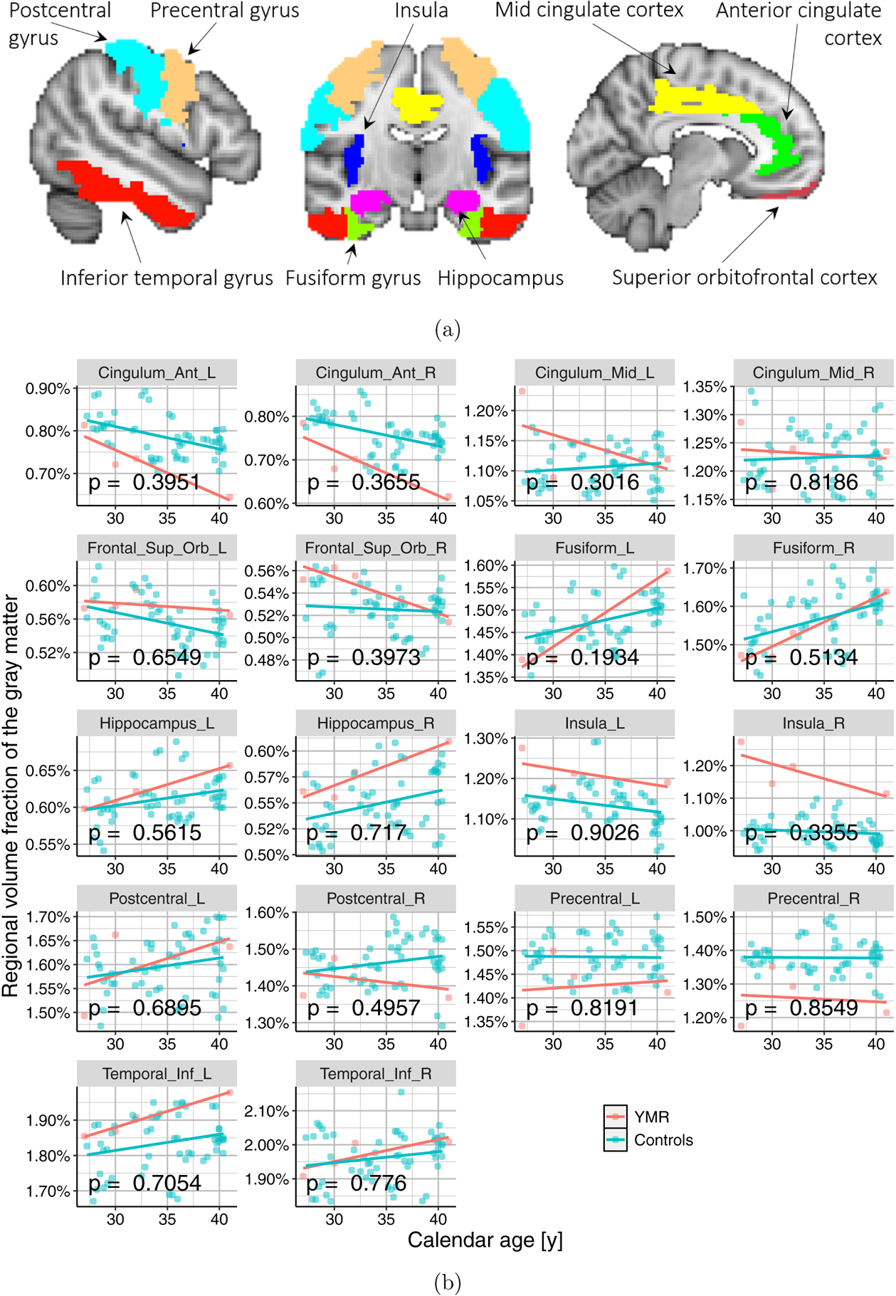
(a) Nine bilateral regions previously implicated in meditation studies (Fox et al., 2014), were selected for the regional volumetric analysis in our case study. These regions were extracted bilaterally, on the left and right hemispheres of the brain, giving us a total of 18 regions per subject. (b) Scatter plots showing the relationship between calendar age and regional volume fraction, for all the 18 regions.

Figure 3.: Overview of the analysis.

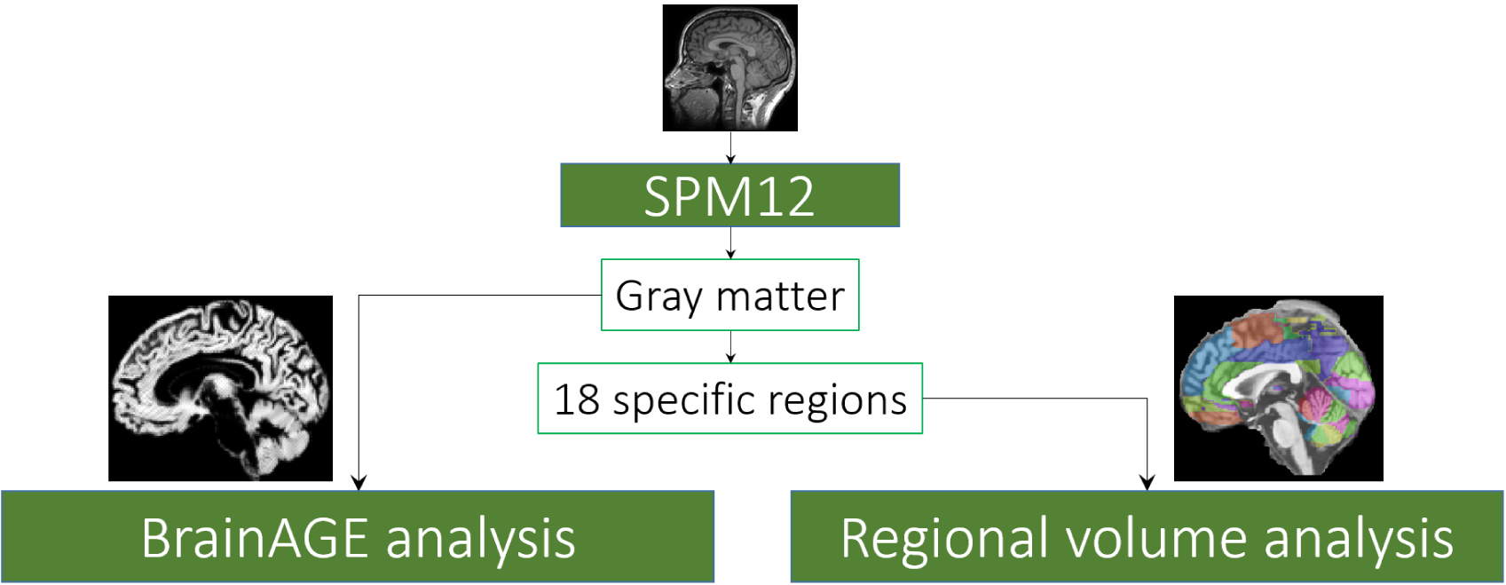
T₁-weighted MRI data were processed through SPM12 to produce gray matter volume maps. These maps were direct inputs for the BrainAGE analysis, and, separately, were segmented for regional volumetric analyses.

Figure 4.: Quality control.

The noise variability of the regional volumes was computed for the data from the years 2002 and 2005, the earliest data available on YMR. The data were acquired on three and two consecutive days, respectively. Variability was low, providing support for the reliability of the data for downstream statistical analysis.

BrainAGE analysis.

Recently, a machine learning-based analysis introduced the Brain Age Gap Estimation (BrainAGE) framework, that can be used to classify the Cartesian space spanned by, the estimated age of the brain using MRI data, and the calendar age (Franke et al., 2013, 2015, 2012, 2014, 2010; Luders et al., 2016). The central conceptual idea of the framework is shown in Fig. 5. The relevance vector machine (RVM) (M. Tipping & Bishop, 2005; M. E. Tipping, 2001; Wei, Yang, Nishikawa, Wernick, & Edwards, 2005) essentially learns a function, f that can predict the age of an input brain image. It learns by finding the best empirical model, relating the whole brain images to the calendar ages. BrainAGE for a particular test subject is the difference between the estimated brain age (BA) and the calendar age (CA), i.e. BrainAGE = BA – CA. This framework has been studied extensively, and has been empirically shown to be robust to variations in scanner parameters (Franke et al., 2010). The analysis was performed using the Spider machine learning toolbox (Weston, Elisseeff, BakIr, & Sinz, 2005).

Figure 5.: BrainAGE estimation framework.

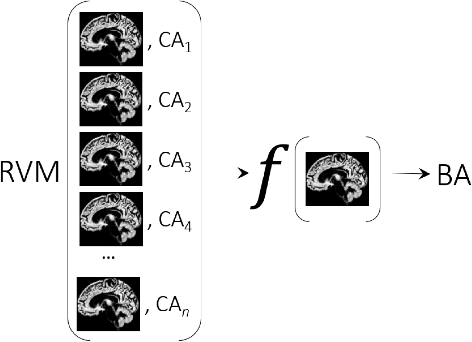
The relevance vector machine (RVM) is used for estimating the age of a brain from MRI data.

The relevance vector machine (RVM) model only consisted of brain voxels as the predictive features. The full brain mask was applied to the swmwc1 files that are produced from the SPM which were directly used as the feature vectors without any additional pre-processing. The voxel size for our images was 1.5 × 1.5 × 1.5 mm³. The number of voxels fed into the relevance vector machine is 962674. The model learns a mapping between brain imaging features (SPM based GM volumes in this case) to the corresponding calendar age. The rest of the sample characteristics are considered in a “second-level” analysis. Thus the RVM model was trained using all the n = 243 samples (in a leave one out fashion) including those of YMR, without using any group or other information. The group analysis was performed after the RVM has been trained agnostic to the groups. Once the brain ages are computed for all the samples, using leave-one-out approach, the following linear model was estimated to assess the statistical significance of slower brain aging in YMR with respect to the controls as well as to the three subgroups of the controls.

$$\text{BA}={\beta }_0+{\beta }_{1}x+{\beta }_2{\delta }_{\text{YMR}}+{\beta }_{3}x{\delta }_{\text{YMR}},$$

where, x denotes the CA and δ is the indicator function for the YMR observations. β₀, the model intercept, denotes the brain age at birth, i.e. x = 0, for the control group. β_l denotes the rate of change in brain age with the respect to the calendar age, i.e. “brain aging” slope, for the controls. β₂ represents the change in the intercept term for YMR compared to controls, and β₃ represents the change in the “brain aging” slope for YMR compared to controls (i.e., an interaction term between group and “brain aging” slope). This linear model is used to assess if the relationship between BA and CA is different for YMR when compared to that of the control population. We also estimate a similar linear model to draw contrast of YMR from the three control subgroups (WL, HEP and MBSR). We would like to note that while such a linear relationship is expected and interpretation about maturation and aging can be drawn from the slopes, the interpretation of brain age at birth is not straight forward and the intercept in this case mainly serves as a nuisance parameter.

Brain resemblance analysis.

The Cartesian space can also be used to provide an estimate of the average calendar age of the control samples, whose brains “resemble” that of YMR at a particular calendar age. It can be computed as follows. Let YMR’s estimated brain age at a particular calendar age CAymr be, ${\widehat{y}}_{\text{YMR}}=f\left(MR{I}_{\text{YMR}}\right)$. Similarly, let $\left\{{\widehat{y}}_i\right\}$ be the set of estimated brain ages ∀i ∈ controls, at their respective calendar ages, {CA_i}. An ordering can be induced onto $\left\{{\widehat{y}}_i\right\}$, such that

$$\left|{\widehat{y}}_1-{\widehat{y}}_{\text{YMR}}\right|\le \left|{\widehat{y}}_2-{\widehat{y}}_{\text{YMR}}\right|\le \dots \le \left|{\widehat{y}}_k-{\widehat{y}}_{\text{YMR}}\right|\le \dots \le \left|{\widehat{y}}_n-{\widehat{y}}_{\text{YMR}}\right|.$$

The first ${\widehat{y}}_1\dots {\widehat{y}}_k$ can be used to compute the average of the corresponding calendar ages CA₁ … CA_k. This analysis can be repeated for different k, to estimate the sensitivity to the choice of k.

Regional volumetric analysis.

The BrainAGE analysis and the brain resemblance analysis both use voxels from the whole-brain gray matter, and reveal the aging of the overall brain. Regional volumetric analyses were conducted to examine if brain aging rate differences could be interpreted in terms of volumetric changes of specific regions, specifically those highlighted in previous meditation research Fox et al. (2014). The average volumes of the 18 regions, as a fraction of total gray matter, were analyzed to test if their rates of change over time are different between YMR and the general population. For each of the 18 regions, a simple linear model, shown below, was fit using data from both the controls⁴ and YMR.

$$v={\beta }_0+{\beta }_{1}x+{\beta }_2{\delta }_{\text{YMR}}+{\beta }_{3}x{\delta }_{\text{YMR}},$$

where, x, like before, denotes the calendar age (CA), v denotes the volume fraction of a region, i.e. the total gray matter volume of a region divided by the total volume of the entire gray matter. Thus it reflects the fraction of the gray matter occupied by a specific region. β₀ represents the starting average volume fraction for controls, i.e. the average volume fraction when x = 0 or equivalently at birth. But, this parameter is harder to interpret since the volumetric changes, beginning from birth, might not be linear. β₁ represents the “regional aging” i.e. the rate of change in the volume fraction of a region with calendar aging, i.e. $(\frac{\partial v}{\partial x})$, for controls. β₂ represents the difference in the intercept for YMR. β₃ represents the difference in the volumetric aging slope for YMR compared to that of controls (i.e. again an interaction term between group and the “volumetric aging” slope).

Statistical analysis.

Since only four measurements were available for YMR, to obtain p-values for the BrainAGE analysis and the regional volumetric analyses, permutation testing with 10, 000 permutations was used to generate the null distributions non-parametrically. In each permutation, the labels of which observations are YMR and Controls were randomly shuffled to reconstitute the size of each group, but enforce the null hypothesis that there is no difference between YMR and Controls, and the statistic of interest is then calculated. The p-value for a test was the proportion of these 10,000 null test statistics that were “as or more extreme” than the associated test statistic obtained from the actual (i.e. non-shuffled) data. For both the BrainAGE and regional volumetric analyses, the null hypothesis H₀ was β₃ = 0, while the alternate hypothesis H₁ for BrainAGE, was β₃ < 0, i.e. YMR’s brain ages slower compared to that of the controls. For the regional volumetric analyses, the H₁ was β₃ ≠ 0, i.e. the volumetric changes over time would be different between the two groups. In other words, for the BrainAGE analysis, it was a one-sided test, while for the regional volumetry, it was two-sided. We would like to note that, for the BrainAGE analysis, as described earlier, the samples in the entire age range were utilized. For the volumetric analysis, which falls under “classical” statistical analysis of examining the significance of differential relationship between calendar age and regional volume, age-matched subsample was used.

3. RESULTS

BrainAGE results.

The BrainAGE framework can be used to classify the space spanned by the estimated brain age and the calendar age, as shown in Fig. 6a. The diagonal arrow can be thought of as representing “typical aging” of the brain, assuming one calendar year equals one brain year. The band represents normal variability in the typical aging of the brain. If the width of the typical aging band is 2γ, then $\text{BrainAGE}<-\sqrt{2}\gamma$ identifies the space below the band, and $\text{BrainAGE}>\sqrt{2}\gamma$ identifies the space above. The bottom space can be further parsed into delayed maturation and delayed aging of the brain, marked by the transition from orange to green. The top space similarly can be parsed into early maturation and early aging of the brain. The transitions between the colors represent “maturation” according to the calendar and the brain ages⁵.

Figure 6.: BrainAGE results.

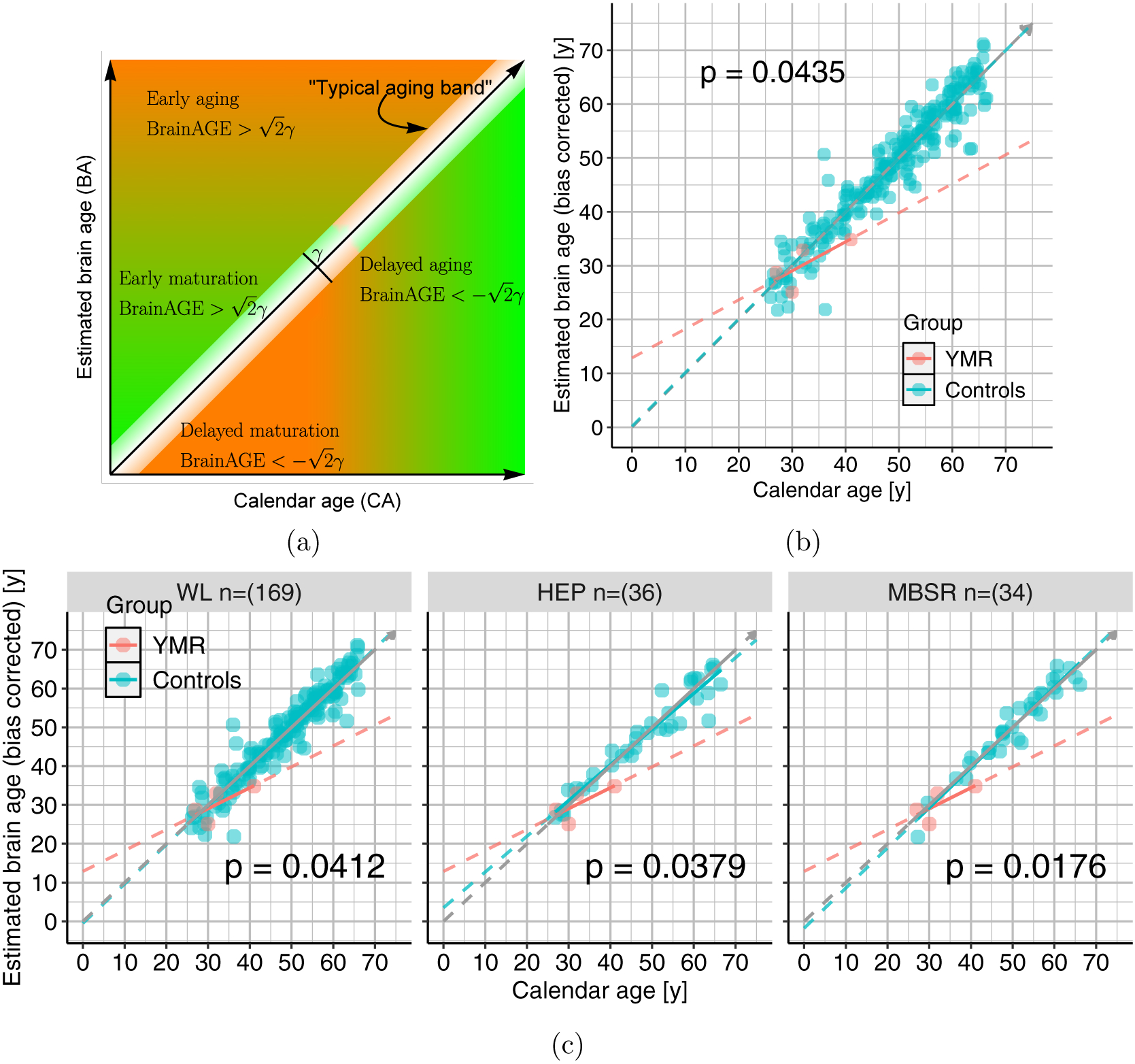
(a) Qualitative classification of the space spanned by estimated brain age and calendar age by BrainAGE (BA – CA). (b) Scatter plot showing the relationship between estimated brain age (BA) and the calendar age (CA) for YMR and the general population. The slope for the general population was β₁ = .99, and the slope difference of YMR was β₃ = −0.45, which was statistically significant at p = 0.0435. (c) Scatter plot showing the relationship between estimated brain age and calendar age contrasting YMR with the three control subgroups. The slope differences with respect to WL, HEP and MBSR are −0.47, −0.38, −0.5, respectively.

Precise interpretation of early maturation in terms of biology is difficult, but if we can use biometric (say gray matter volume) that has a growth and decay phase based on the brain age (BA) (Fig. 7 (left)), and one can interpret certain points in those phases as beginning maturation (say gray matter volume crossing a certain threshold) and beginning of aging (say gray matter volume crossing a certain decline threshold), then those points can be mapped to the calendar age axis (Fig. 7 (right). Depending on the slopes and the crossing point with the diagonal, the maturation and aging points on the calendar age can be shifted. The notion of both early maturation and delayed aging are based on extrapolations of the linear model(s) and its (their) intersection with the diagonal line (Fig. 7). If the typical maturation happens before the crossing point, then we can interpret the reduced slope with early maturation (left shift on the calendar age indicated by the gray arrow). If the typical aging begins after the crossing point then we can interpret the reduced slope with delayed aging (right shift on the calendar age indicated by the gray arrow). Though we do not actually have the true cut offs (dotted gray lines), it is estimated that typical maturation occurs at around 25 years of calendar age (Casey, Getz, & Galvan, 2008). Since the demarcations on Fig. 6(a) are based on the cut off and are critical to understand these distinctions, and it is far from trivial to obtain those demarcations, we used the term “qualitatively” for such interpretations. Furthermore, while slopes of such a linear model can be used to draw interpretations about maturation and aging, the interpretation of brain age at birth, i.e. CA=0 is not straight forward, and the BA-intercept mainly serves as a nuisance parameter.

Figure 7.:

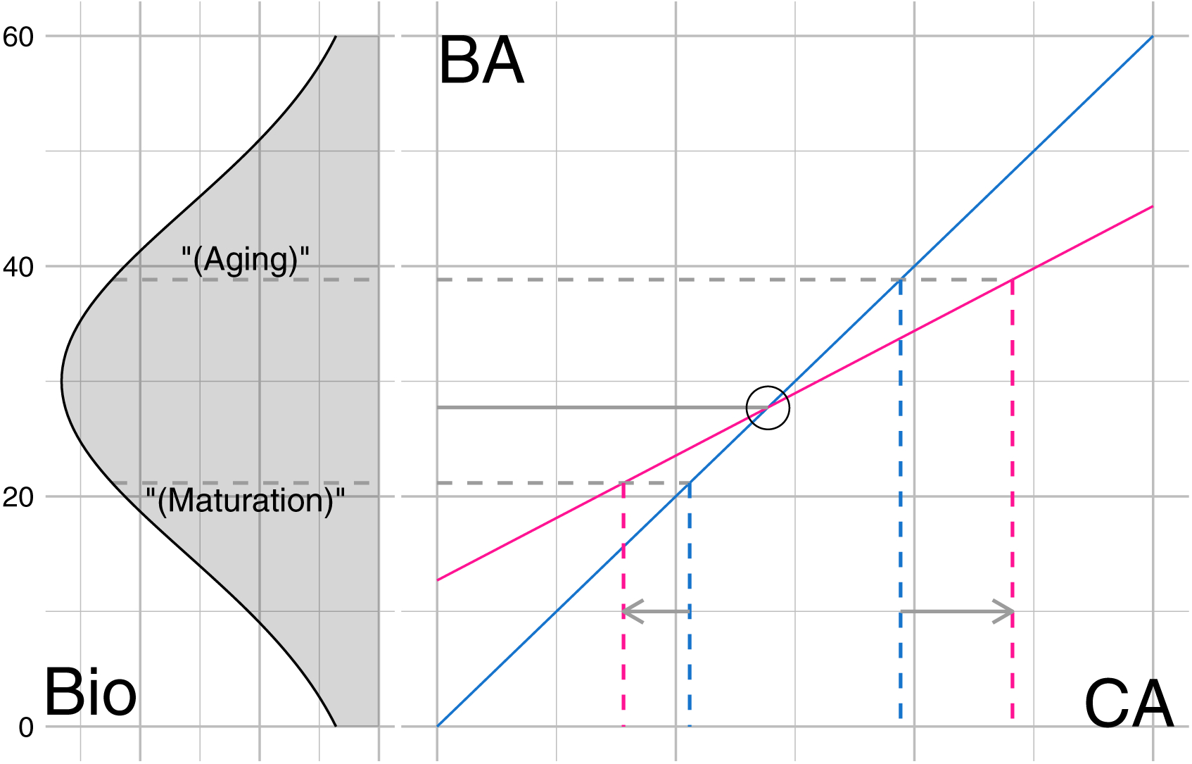
Conceptual graphic to demonstrate maturation and aging points. Left: growth and decay of some biological feature (Bio) (say gray matter volume) with the brain age (BA). Right: Depending on the relationship of the brain age with the calendar age, the maturation and aging points projected onto the calendar age (CA) can be shifted to the left (early maturation) or to the right (delayed aging).

The relationships between estimated brain age and calendar age for YMR and the control sample are shown in Fig. 6. Together, these plots qualitatively indicate that YMR’s brain ages slower than his calendar age, and that his brain demonstrates early maturation but delayed aging, while the controls fall in the “typical aging band”. Quantitatively, the brain aging slopes for YMR and the general population are β₁ = 0.99, respectively, and their difference, β₃ = −0.45 is statistically significant at p = 0.0435, implying YMR’s brain aging rate is slower than that of the general population, in the time window sampled for YMR.

Effects of bias correction.

We have also applied the bias correction based on Eq. 1 in the paper (Beheshti et al., 2019). The effect of bias correction is apparent in plots of Figs. 8 and 9. The prediction performance using mean absolute error (MAE), root mean squared error (RMSE) and R² is also reported in Table 1.

Figure 8.: Effects of bias correction.

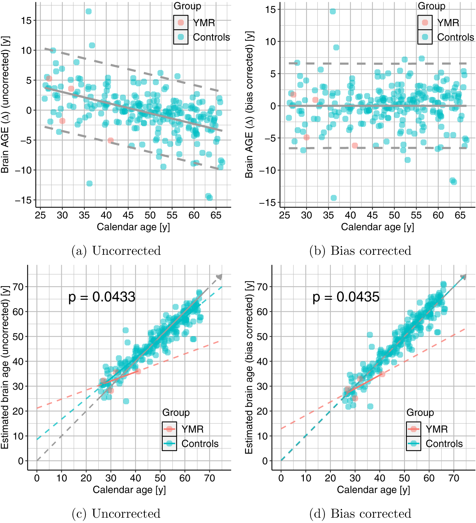
Scatter plots showing relationship between the calendar age (CA) and (top-panel:) BrainAGE (age gap estimation Δ) and (bottom-panel:) estimated brain age (BA). We can clearly see that the inverse relationship between Δ and CA is no longer present after the correction and the models in the bottom panel tend toward the diagonal. The p-value for the group difference test is only modestly affected.

Figure 9.: Effects of bias correction.

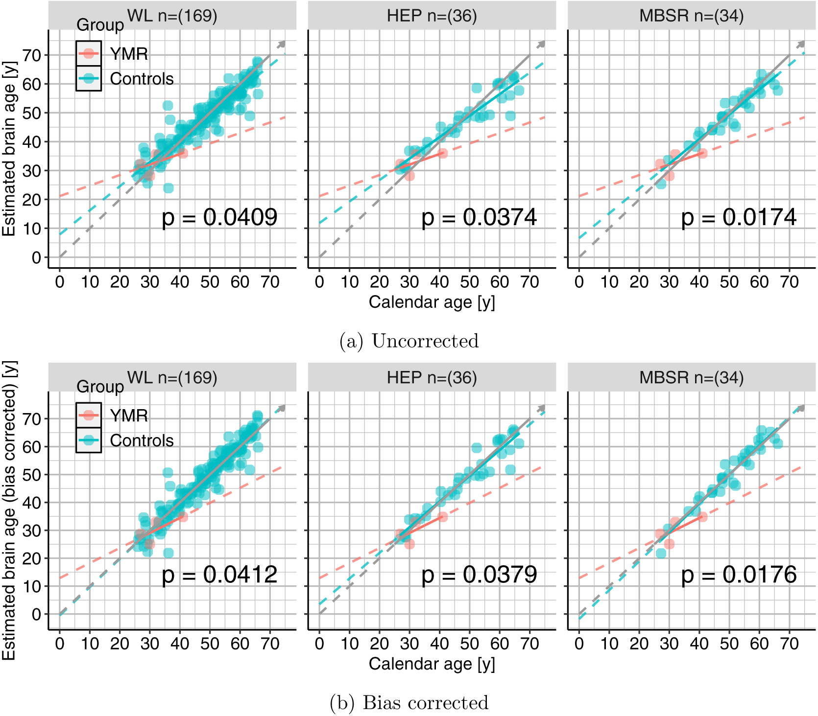
Plots similar to the bottom panel of Fig. 8 but for each of the three subgroups of controls. Top-panel shows those for uncorrected data and the bottom-panel shows the results with bias corrected data. We can again see that the linear models move towards the diagonal in all the three subgroups and p-values only modestly affected.

Table 1.:

Prediction performance of bias correction method (Beheshti et al., 2019) applied to our data.

	Uncorrected	Bias corrected
MAE	2.676096 [y]	2.345017 [y]
RMSE	3.810205 [y]	3.300468 [y]
R2	0.8820153	0.9156289

Brain resemblance results.

As shown in Fig. 10b, the brain resemblance of YMR was computed using seven different values of k. It was found that his brain at 41 years “resembled” that of a 33.06 ± 0.60 years old subject from this control population. The analysis was also repeated at his calendar age of 27, 30 and 32 years. The corresponding brain resemblances are shown in Table 2.

Figure 10.: Brain resemblance results.

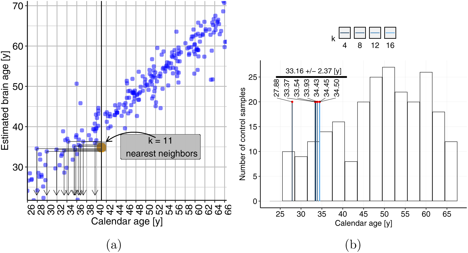
(a) Demonstration of the brain resemblance calculation, using k = 11, for YMR’s calendar age of 41 years. The blue scatter is from the control sample, and the orange dot shows YMR at 41. (b) The brain resemblance results, for seven different ks. The histogram of the calendar ages of the controls, on the back drop, shows the wide range of the age sample distribution, indicating that k-nearest neighbor search is not biased towards younger ages.

Table 2.:

Brain resemblance results for the four different calendar ages of YMR.

YMR calendar age [y]	Control calendar age [y]
27	30.29±1.43
30	28.23 ± 0.64
32	32.34 ± 0.59
41	33.16 ± 2.37

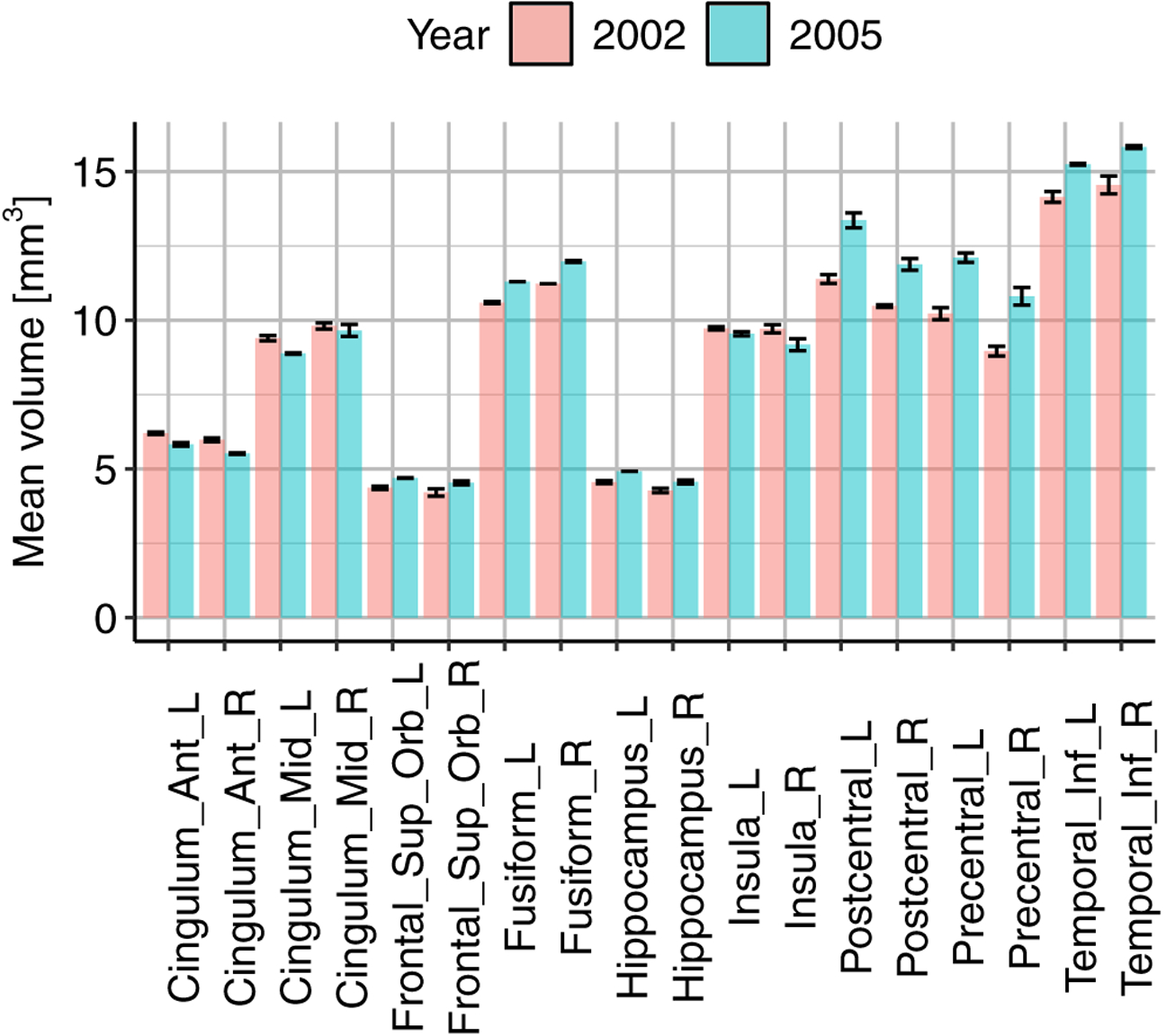
Regional volumetric analysis results.

The results shown in Fig. 11, indicate that for all the regions, the rate of change (i.e. shrinkage vs. expansion over time) of volume fraction, is not statistically different between YMR and this control population. These results, together with the result in Fig. 6c, demonstrate that the “brain aging” patterns may not simply be revealed by studying gross volumetric changes of specific regions, and that using machine learning based predictors on the high-dimensional MRI images may provide better evaluation of brain aging, since such an approach can capture coordinated changes spanning across the entire brain.

4. DISCUSSION

Given recent interest in the potential effects of meditation on brain aging, we sought to examine the aging profile of expert meditator YMR’s brain in comparison to that of the general population. To do this, we made use of the BrainAGE machine learning predictor, which computes an individual’s brain age based on levels of gray matter throughout the brain, and allows assessment of the difference between the individual’s brain age and calendar age. We collected T₁-weighted MRI scans of YMR’s brain at four time points between 2002 and 2016, and collected scans from 105 control subjects to train the BrainAGE predictor. We found that, first, YMR’s brain age advanced at a slower rate than his calendar age, and his brain aging rate was significantly slower than that of the general population. Qualitatively, YMR’s brain indicated early maturation but delayed aging. Second, YMR’s brain, based on his latest scan in 2016 at calendar age 41, resembled that of an average 33-year-old’s from the general population. However, this large resemblance gap was not observed for YMR’s earlier age scans (i.e. ages 27, 30 and 32), potentially suggesting that any delayed aging may only begin to manifest at older ages. Third, we did not find differences between YMR and the general population in gross volumetric changes over time in the regions of interest, suggesting that the detected brain aging differences may arise from more subtle gray matter changes spread throughout the whole brain.

The findings from this unique longitudinal data set of an expert meditator add to a growing literature that suggests that meditative practice may be associated with slowed biological aging (Chaix et al., 2017; Lazar et al., 2005; Luders et al., 2016, 2015; Pagnoni & Cekic, 2007). The results prompt more systematic longitudinal evaluation of the relationship between extensive meditation practice and brain aging.

Limitations.

Broadly, it is important to emphasize that several factors besides meditation may be playing a role in YMR’s relatively slowed brain aging. Our study is not equipped to assess whether there is a direct relationship between YMR’s brain aging profile and his meditative practice. Furthermore, the BrainAGE predictor used here to determine YMR’s brain age was trained on Americans whose overall lifestyles and environment through development likely differed from YMR’s. It would be of interest in future studies to train the BrainAGE predictor on non-meditators from Tibet to obtain a more rigorously-matched control sample.

On a technical level, while the imaging data were acquired at the same site for all of YMR’s visits and for all of the control subjects, there was a scanner upgrade in 2010. Nonetheless, image processing was accompanied by the same quality-control measures for all scans, and all scans were preprocessed through the same, standardized SPM pipeline, which collectively should minimize the effects of scanner differences. Finally, the accuracy of the machine learning predictor can have a non-trivial effect on identifying and understanding the relationships between brain aging and calendar aging. The relevance vector machine (RVM) mitigates the “curse of dimensionality” by regularizing the actual number of parameters needed to be estimated, thus encouraging generalizability of the learnt model. As discussed in the original work (M. E. Tipping, 2001), RVM picks much smaller set of basis functions compared to the support vector machines. That is the number of relevant vectors does not grow linearly with training set as the support vectors do. This is due to the sparsity inducing prior on the weights p(w_i) (Student-t vs. Gaussian Eq. 32 in M. E. Tipping (2001)), equivalently viewed as penalizing ${\sum }_i\text{log}\left|w_i\right|$ (Eq. 33 in M. E. Tipping (2001).) While relevance vector machines (RVMs) used in this work offer reasonable accuracy, future analyses may benefit from using newer, deep-learning based predictors that may offer better accuracy in modeling these relationships.

References

- Alda M, Puebla-Guedea M, Rodero B, Demarzo M, Montero-Marin J, Roca M, & Garcia-Campayo J (2016). Zen meditation, length of telomeres, and the role of experiential avoidance and compassion. Mindfulness, 7(3), 651–659. [DOI] [PMC free article] [PubMed] [Google Scholar]
- Ashburner J, & Friston KJ (2000). Voxel-based morphometrythe methods. Neuroimage, 11 (6), 805–821. [DOI] [PubMed] [Google Scholar]
- Beheshti I, Nugent S, Potvin O, & Duchesne S (2019). Bias-adjustment in neuroimaging-based brain age frameworks: A robust scheme. NeuroImage: Clinical, 24, 102063. [DOI] [PMC free article] [PubMed] [Google Scholar]
- Casey BJ, Getz S, & Galvan A (2008). The adolescent brain. Developmental review, 28(1), 62–77. [DOI] [PMC free article] [PubMed] [Google Scholar]
- Chaix R, Alvarez-López MJ, Fagny M, Lemee L, Regnault B, Davidson RJ, … Kaliman P (2017). Epigenetic clock analysis in long-term meditators. Psychoneuroendocrinology, 85, 210–214. [DOI] [PMC free article] [PubMed] [Google Scholar]
- Cole JH, Ritchie SJ, Bastin ME, Hernandez MV, Maniega SM, Royle N, … others (2018). Brain age predicts mortality. Molecular psychiatry, 23(5), 1385. [DOI] [PMC free article] [PubMed] [Google Scholar]
- Epel E, Daubenmier J, Moskowitz JT, Folkman S, & Blackburn E (2009). Can meditation slow rate of cellular aging? cognitive stress, mindfulness, and telomeres. Annals of the new York Academy of Sciences, 1172(1), 34–53. [DOI] [PMC free article] [PubMed] [Google Scholar]
- Fox KC, Nijeboer S, Dixon ML, Floman JL, Ellamil M, Rumak SP, … Christoff K (2014). Is meditation associated with altered brain structure? a systematic review and meta-analysis of morphometric neuroimaging in meditation practitioners. Neuroscience & Biobehavioral Reviews, 43, 48–73. [DOI] [PubMed] [Google Scholar]
- Franke K, Gaser C, Manor B, & Novak V (2013). Advanced BrainAGE in older adults with type 2 diabetes mellitus. Frontiers in aging neuroscience, 5, 1–9. [DOI] [PMC free article] [PubMed] [Google Scholar]
- Franke K, Hagemann G, Schleussner E, & Gaser C (2015). Changes of individual BrainAGE during the course of the menstrual cycle. NeuroImage, 115, 1–6. [DOI] [PubMed] [Google Scholar]
- Franke K, Luders E, May A, Wilke M, & Gaser C (2012). Brain maturation: predicting individual BrainAGE in children and adolescents using structural MRI. NeuroImage, 63(3), 1305–1312. [DOI] [PubMed] [Google Scholar]
- Franke K, Ristow M, & Gaser C (2014). Gender-specific impact of personal health parameters on individual brain aging in cognitively unimpaired elderly. Frontiers in aging neuroscience, 6, 1–14. [DOI] [PMC free article] [PubMed] [Google Scholar]
- Franke K, Ziegler G, Klöppel S, Gaser C, Initiative ADN, et al. (2010). Estimating the age of healthy subjects from t1-weighted MRI scans using kernel methods: Exploring the influence of various parameters. NeuroImage, 50(3), 883–892. [DOI] [PubMed] [Google Scholar]
- Kurth F, Cherbuin N, & Luders E (2017). Promising links between meditation and reduced (brain) aging: an attempt to bridge some gaps between the alleged fountain of youth and the youth of the field. Frontiers in Psychology, 8, 860. [DOI] [PMC free article] [PubMed] [Google Scholar]
- Lazar SW, Kerr CE, Wasserman RH, Gray JR, Greve DN, Treadway MT, … others (2005). Meditation experience is associated with increased cortical thickness. Neuroreport, 16 (17), 1893. [DOI] [PMC free article] [PubMed] [Google Scholar]
- Le Nguyen KD, Lin J, Algoe SB, Brantley MM, Kim SL, Brantley J, … Fredrickson BL (2019). Loving-kindness meditation slows biological aging in novices: Evidence from a 12-week randomized controlled trial. Psychoneuroendocrinology. [DOI] [PubMed] [Google Scholar]
- Luders E, Cherbuin N, & Gaser C (2016). Estimating brain age using high-resolution pattern recognition: younger brains in long-term meditation practitioners. Neuroimage, 134, 508–513. [DOI] [PubMed] [Google Scholar]
- Luders E, Cherbuin N, & Kurth F (2015). Forever young (er): potential age-defying effects of long-term meditation on gray matter atrophy. Frontiers in Psychology, 5, 1551. [DOI] [PMC free article] [PubMed] [Google Scholar]
- Pagnoni G, & Cekic M (2007). Age effects on gray matter volume and attentional performance in zen meditation. Neurobiology of aging, 28(10), 1623–1627. [DOI] [PubMed] [Google Scholar]
- Schutte NS, & Malouff JM (2014). A meta-analytic review of the effects of mindfulness meditation on telomerase activity. Psychoneuroendocrinology, 42, 45–48. [DOI] [PubMed] [Google Scholar]
- Tipping M, & Bishop C (2005, April 12). Variational relevance vector machine. Google Patents. (US Patent 6,879,944)
- Tipping ME (2001). Sparse bayesian learning and the relevance vector machine. Journal of machine learning research, 1 (June), 211–244. [Google Scholar]
- Wei L, Yang Y, Nishikawa RM, Wernick MN, & Edwards A (2005). Relevance vector machine for automatic detection of clustered microcalcifications. IEEE transactions on medical imaging, 24 (10), 1278–1285. [DOI] [PubMed] [Google Scholar]
- Weston J, Elisseeff A, BakIr G, & Sinz F (2005). The spider machine learning toolbox. Resource object oriented environment. Available at: http://people.kyb.tuebingen.mpg.de/spider/main.html [accessed December 2011]. [Google Scholar]
Associated Data
This section collects any data citations, data availability statements, or supplementary materials included in this article.