Lagged Correlations among Physiological Variables as Indicators of Consciousness in Stroke Patients

Abstract

Consciousness is a highly significant indicator of an ICU patient’s condition but there is still no method to automatically measure it. Instead, time consuming and subjective assessments are used. However, many brain and physiologic variables are measured continuously in neurological ICU, and could be used as indicators for consciousness. Since many biological variables are highly correlated to maintain homeostasis, we examine whether changes in time lags between correlated variables may relate to changes in consciousness. We introduce new methods to identify changes in the time lag of correlations, which better handle noisy multimodal physiological data and fluctuating lags. On neurological ICU data from subarachnoid hemorrhage patients, we find that correlations among variables related to brain physiology or respiration have significantly longer lags inpatients with decreased levels of consciousness than in patients with higher levels of consciousness. This suggests that physiological data could potentially be used to automatically assess consciousness.

Introduction

Patients in intensive care units (ICUs) are extremely challenging to treat given the complex, critical, and changing nature of their conditions. Each patient’s state fluctuates over time, due to recovery or worsening, and as a result of interventions. However it can be difficult to gain insight into this state, and to identify factors that can be intervened upon to improve outcomes. That is, clinicians need to understand not only what is happening but why it is happening. One of the most fundamental factors influencing treatment decisions and predictions of prognosis in an ICU is a patient’s state of consciousness. Despite the critical nature of this information, there is not yet a way to measure consciousness automatically. Instead, clinicians administer labor-intensive tests such as the Glasgow Coma Scale (GCS)¹, often only once a day. These subjective daily assessments make it difficult to determine causes and effects of consciousness, which may also fluctuate between assessments. Instead, if consciousness could be measured automatically and continuously, this would have both clinical impact (better understanding of prognosis, earlier identification of changes in consciousness, and reduced burden on clinicians) and research implications (more frequent assessments would enable analysis of causes and effects of consciousness).

While consciousness is still poorly understood, ICUs now routinely collect large amounts of data that can provide insight into a patient’s state. Multimodality monitoring including EEG, cardiovascular parameters, and brain physiology is now being increasingly used to guide clinical care in ICU,² and for research predicting ICU outcomes.³ Despite the success of machine learning in analyzing ICU data, there has not yet been an effort to use routinely collected ICU data to gain insight into consciousness. We focus in particular on automated detection of factors related to consciousness in stroke patients in the neurological intensive care unit (NICU), due to the severity of illness and potential for improving care with a better understanding of consciousness. While data in the NICU is high frequency (often at a resolution of 5 seconds), there are many challenges in using this data to automatically detect consciousness, including the need to combine multiple sensing modalities and identify sometimes subtle signals within noisy data. First, different variables are measured for different patients, necessitating methods that do not require all possible variables to be present. Similarly, we expect different levels of consciousness to manifest indirectly across features in multiple variables. Since consciousness is assessed infrequently (generally once a day), there are few training labels, which poses a challenge for most classification methods. On the other hand, these labels also make it difficult to treat the problem as one of changepoint detection (determining when the system’s parameters or structure change), since we do not know precisely when a change occurred (e.g. if consciousness is high on Monday morning, and low on Tuesday morning we do not know when the change happened in between).

Instead, we propose that multimodality monitoring (MMM) can be used to gain insight into consciousness, by examining lagged correlations between the measured variables. We hypothesize that since many biological variables are correlated, when consciousness is interrupted, these correlations may be too. Thus, rather than use raw MMM data directly, we propose that the time lag of correlations is a highly informative feature. While prior methods exist to identify lagged correlations, we introduce the first method to identify when the lag between correlated variables changes, and to do so in multimodality data while being robust to noise. We build on cross-correlation, which is widely used to find the lags (delays) in time series⁴, introducing a new approach that can identify when lags change over time. We further contribute a kernel that is better suited to multimodality physiological data (allowing identification of more subtle relationships), and an optimization procedure to identify lags across an entire time series (e.g. patient’s ICU stay) while being robust to noise and outlying values. Experimentally, we show that this method can accurately recover true changing lags on simulated data, while existing work that does not account for changes has significantly lower accuracy. Finally, we apply the approach to a set of NICU data from 61 patients with subarachnnoid hemorrhage (SAH), identifying biologically plausible relationships. In particular, we find that brain and cardiovascular variables are correlated with shorter delays in patients with high versus low levels of consciousness.

The primary contributions of our work are:

1. We motivate the use of lagged correlations for gaining insight into biomedical data.

2. We introduce nonstationary normalized cross-correlation (N²C²), a new method for automatically identifying lagged correlations whose timing may change over time. This highly general approach may be applicable to many types of biomedical time series, as well as time series more generally.

3. We apply N²C² to NICU data and demonstrate novel differences in lags that appear to depend on state of consciousness.

Our approach provides a first step toward both better use of high-frequency ICU data to gain insight into previously invisible patient states, as well as a better and more objective understanding of consciousness in the ICU.

Related Work

Consciousness is a fundamental and yet unsolved problem in biology.^5,6 Most studies of consciousness focus on EEG and fMRI data,⁷ but this does not allow continuous measurement in the ICU. In the ICU, consciousness is generally assessed with qualitative instruments such as the Glasgow Coma Scale (GCS)⁸ and Alert, Voice, Pain, Unresponsive (AVPU) scale.⁹ Recent studies have shown that consciousness rests on the brain’s ability to sustain rich brain dynamics¹⁰ and metastability in brain dynamics can be used to understand altered levels of consciousness.¹¹ There have been some efforts using bedside EEG to predict changes in consciousness in stroke patients,¹ and using network dynamics to distinguish comatose from healthy patients using EEG.¹² Other efforts have used EEG data to identify differences in sleep patterns between patients with different states of consciousness.¹³ However, we are not aware of work using this data to detect the current state of consciousness in real-time.

On the other hand, machine learning analysis of ICU data has focused on predicting readmission¹⁴ or ICU outcomes³ and classifying physiological features to identify disorders.¹⁵ Yet, physiological data has been shown to provide insight into brain activity, such as in a recent study that identified correlations between physiological signals (including respiration, CO2 levels in blood, heart rate) and fMRI-monitored brain connectivity.¹⁶ Other works showed that delayed cerebral ischemia after SAH could be predicted from physiological time series data.¹⁷ Thus, it is possible that physiological data could provide a window into not only clinical outcomes, but also brain function and potentially consciousness. We hypothesize that time lags between variables may be an important signal. For example, lags in resting state fMRI and EEG provided insight into neuronal processes,¹⁸ and lags are widely studied among physiological data more generally, including in analysis of electrodermal activity¹⁹. One of the most common methods for examining such lagged relationships is cross-correlation, which has been applied to local field potentials to gain insight into brain regions²⁰. Cross-correlation is a measure of similarity between two time series. For two time series with identical values, where one is a shifted version of the other, correlation will be highest, with a value of 1. To identify the lag with the maximal correlation for a pair of variables, essentially one time series is iteratively shifted with the correlation being repeatedly computed. Cross-correlation has been used for time delay estimation,^21,22 such as for finding the phase shift between acoustic signals, but this aims to find the shift between two measurements of the same process, whereas our variables capture different processes that may causally influence one another.

While there are many extensions to cross-correlation, including faster to compute and normalized versions,^23–25, it still poses problems for biological time series. First, it is assumed that the lag is the same for the entire time series, which is unlikely to be true for a patient whose physiology and state is changing – particularly in the ICU. Second, even during times of relative stability, there are smaller fluctuations due to both physiology as well as the noise and error inherent in biomedical data. By assuming a single lag, these approaches may be susceptible to the effects of outlying values. While some works have applied cross-correlation to nonstationary time series, they have done so by first removing the trends in the data to make it stationary,²⁶ whereas we propose that the trends are highly informative in ICU and other physiological data where we aim to uncover the causes of changes in state. Most fundamentally, there is currently no method that can identify when and how the lags between variables change over time. We propose that this is a critical signal for assessing consciousness, and methods for finding changes in lagged correlations may have many applications to the other types of health data described above.

Method

As a first step toward automated assessment of consciousness, we focus on identifying how time lags between correlated variables change as a function of consciousness. To do this using physiological data routinely collected in ICU, we introduce a new method, N²C² (nonstationary normalized cross-correlation), based on normalized cross-correlation (NCC), that identifies when and how the lags between variables changes over time. Unlike the state of the art, which assumes the lag between two time series remains constant, this allows us to identify both gradual shifts in time lag (e.g. slow change from 1 to 5 second lag) as well as sudden transitions (e.g. such as after an intervention). Further, this indirectly provides detection of changepoints, but with more context (i.e. what is changing) and more flexibly (i.e. not requiring a change to be in the mean of a variable’s value), than the state of the art without the need for specifying a model as in many prior works.²⁷ Thus our output may be that from hour 0 to hour 10 heart rate (HR) and respiration rate (RR) are synchronized with a lag of 0, while from hour 10 to 12, RR lags HR by 1 minute. By testing how the lags differ across patients in different states of consciousness, we can learn characteristics of these states, which could be used for detecting an individual’s current level of consciousness and further when it changes (e.g when the lag between certain variables grows). Figure 1 shows an overview of the procedure.

Figure 1:

This figure shows an overview of the proposed method. First, we set the length of time window, W. Then, sliding this time window across the series we search over each lag l in the set of possible lags between A and B. To identify which lags are significant, we use a permutation test. To ensure lags change smoothly and are not sensitive to outlying values, we determine the lags for the entire time series at once, using the 3D surface shown. Finally, we output a sequence of lags for variables A and B. In this example, the lags increase non-monotonically across time, with B having an increasingly delayed response to A’s value.

We build upon NCC, which is more interpretable than cross-correlation and can handle variables with varying ranges. This is particularly important for MMM data, where variables differ substantially in range, standard deviation, and frequency. NCC is defined as:

$$NCC\left(x,y,l\right)=\frac{{\displaystyle {\sum }_{t\in T}\left(x[t]-\overline{x}\right)\left(y[t+l]-\overline{y}\right)}}{\sqrt{{\displaystyle {\sum }_{t\in T}{\left(x[t]-\overline{x}\right)}^2}}\sqrt{{\displaystyle {\sum }_t{\left(y[t+l]-\overline{y}\right)}^2}}}$$ (1)

where x and y are time series with the same measurement frequency, T is the time series, and l the lag being tested. NCC(x, y, l) is then the correlation between x and y where y is shifted B time steps. While NCC can tell us how related two time series are and with what lag, it has the fundamental limitation that the time lag is constant across time.

N²C²: finding changing lags over time

We now introduce nonstationary normalized cross-correlation (N²C²), which identifies changes in lagged correlations for a set of time series data D. In the case of physiological data, the lags may differ between patients, or within a patient over time (e.g. due to an intervention or change in status). Lags further can fluctuate over time both due to the underlying biology as well as our noisy measurements of it. Thus some seeming changes may be due to relationships that have a time window (e.g. variation within 1-5 min). If we simply accepted the most significant lag at each timepoint, we could then find frequent oscillation between 1 and 5 minutes, even though there is no actual change. To address this we make two key assumptions:

Assumption 1 Lags between physiological variables in ICU tend to zero.

Assumption 2 True lags have higher NCC and at a short timescale, lags are stable.

Assumption 1 says that if all else is equal, we believe that shorter lags are more biologically plausible in our application areas. For other applications the reverse may be true, such as when there is a known delay in information transmission. Assumption 2 says that if we find a lag, say, of 3 seconds between HR in a patient’s data at time 0, a lag of 0 at time 1, and lag of 3 seconds for times 2-10, despite assumption 1, the lag at time 1 is unlikely to be zero because we believe lags are locally stable. By stable we mean that having smaller or no changes in lags is more probable than large changes. In practice we may find multiple lags with similar significance levels (perhaps lag 0 was only slightly more significant than 3 at that time), and this is used to ensure smooth transitions at short timescales. While this ensures some smoothness in lags, by examining lags as forming a continuous surface we are still able to identify when there is a change in the trend, such as if lags shift from an average of 0 to an average of 3 over time.

Step 1: Finding potential lags In general, we focus on finding relationships between all pairs of variables x, y in either direction (with x lagging y or vice versa), though this set could be constrained for example when it is known that the correlation must be in one direction or the other. For instance, if we want to find the speed of the sound in a certain material then knowledge of the microphones’ positions can be used to inform the direction of each lag (as it should be from the microphone closest to the source to the others). Note that treating each direction separately (finding the most likely lag from x to y and vice versa) enables us to find the lags for each stage of a feedback loop. We assume the data D is a v × T matrix, where D(x, i) is the value of variable x at time i. We are able to calculate correlation when some portion of the data are missing, however we also apply methods that have been developed for imputing missing values in ICU and biomedical data to reduce the degree of missingness²⁸.

More formally, we aim to identify lags that change over time, so we first partition the time series into a set of overlapping windows of size w, with the step size being the measurement frequency (i.e. the window advances by one unit at each step). The parameter w should be chosen to be small enough that lags are likely to remain stable within this period (so w should be smaller in data that changes rapidly rather than in systems that are more stable), while being large enough that there are enough measurements to accurately calculate the NCC. While the choice of w is important, it mainly should be chosen to reflect the scale at which changes are happening, and is not sensitive to small differences. For the ICU data in this paper, we select a w of 300 minutes (5 hours), since we use data at a resolution of 1 minute. Since there can be many local fluctuations, with a shorter window it becomes more challenging to identify the overall patterns in this noisy data.

Within each window, we iterate over the set of potential lags l ∈ [0, l_max], calculating NCC(x, y, l) using only the data in the window (as again the lag may change over time). That is, for each pair of variables x and y in D for each window w, we iterate over the lags to form the set of scores:

$$N^2{C}^2\left(x,y,t,w\right)[l]=\frac{{\displaystyle {\sum }_{i\in \left[t-w,t+w\right]}\left(x[i]-\overline{x}\right)\left(y[i+l]-\overline{y}\right)}}{\sqrt{{\displaystyle {\sum }_{i\in \left[t-w,t+w\right]}{\left(x[i]-\overline{x}\right)}^2}}\sqrt{{\displaystyle {\sum }_t{\left(y[i+l]-\overline{y}\right)}^2}}}.$$ (2)

The output is for the window centered at time t, a vector of l_max with correlation scores for each lag. By repeating this for each time t ε T, we have a set of vectors covering the entire time series. Unlike NCC, this uses a subset of the data (rather than the whole time series) at each step, and rather than identify the maximum correlation, outputs the score for all lags.

Step 2: Assessing significance of lags As we have stressed, one of the challenges posed by biomedical data is that lags between variables may fluctuate without there being a significant change in the relationship between variables, such as due to noise, measurement error, or relationships with time windows rather than single lags among other reasons. Thus we cannot simply select the lag with the highest correlation at each t, as this may lead to undesirable properties across the time series, namely a violation of our assumption of local stability of lags. To address this, we first identify which correlations are statistically significant, then from that set optimize for a set of smoothly changing lags across the entire time series.

First, not all tested variables will be correlated, so we must determine which pairs (and at which lags) to accept. Since it can be challenging to determine a null hypothesis, we use a permutation test to find the null and then determine which correlations are significant compared to that. The permutation test shuffles the times associated with one variable’s data within the tested window and then recomputes the correlation. The idea is that by breaking the temporal sequence of the data, we can then learn the distribution of scores for time series that are uncorrelated. This is repeated S times to obtain a distribution of correlation scores for uncorrelated data. In this work we use an S of 200. Using this, we can determine if, compared to this null distribution, our observed results are statistically significant. The result of this step is a subset of the lags from the first step (those determined to be significant), though there may still be multiple significant lags at each time for each variable pair.

To find the single most likely lag for each pair x, y at each time t ε T we apply a kernel to give higher weight to shorter lags (as in our assumptions), and then identify lags using the entire sequence of scores. First, we apply a stretched tricube kernel to N²C²(x, y, t)[]. We use only the positive side of the kernel (0 < u < 0.5) in:

$$K\left(u\right)=\frac{70}{81}{\left(1-|u{|}^3\right)}^3.$$ (3)

As a result, we have a kernel that encodes a preference for lags closer to zero while still allowing the possibility of longer lags. Figure 2 shows the tricube kernel and our stretched version. As shown, our kernel has the same preference for shorter lags, but decreases more slowly as the lag increases, allowing for identification of longer lags. In this setting, negative lags are captured by testing both N²C²(x, y, t) and N²C²(y, x, t), which further allows identification of feedback relationships.

Figure 2:

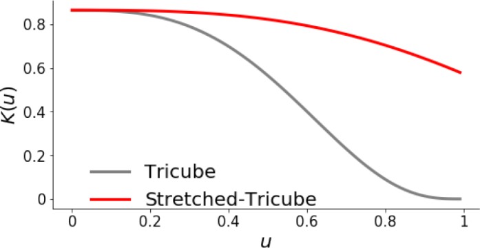
Tricube kernel and stretched tricube kernel. Both kernels have the highest weight near zero, but the stretched kernel drops less dramatically, allowing identification of longer lags.

The kernel encodes assumption 1 (shorter lags are more plausible), but still leaves us with a number of lags at each timepoint. To select between these, we now formulate this as an optimization problem using assumption 2. After applying the kernel, we concatenate each N²C²(x, y, t)[] vector. This leads to a matrix of size T × lmax, ^with lmax being the maximum tested lag. Each entry of the matrix is the associated N²C² score. We can visualize the result as a 3D surface, as shown in figure 1. Intuitively, to select the sequence of lags [0,T] we aim to find the optimal path through the surface. The optimal path is one that maximizes significance while minimizing distance (to avoid large jumps). This optimization problem (max significance, min distance, with a preference for smaller lags as in assumption 2) is akin to voting, and can be solved using the Borda count, applied to sliding windows. Borda count gives a higher ranking to higher correlations and voting among the adjacent lags leads to a stable transition, which fulfills assumption 2. Note that the count is applied to a sliding window (here of length 10, which is sufficiently large to ensure smoothness, while being small enough to allow for changes in lags), which allows for transitions and changes in lags whereas applying it to the entire time series would force consensus. After using Borda count, we have a single series of length T, with the lags between variable x and y. Note that the series of lags can be discontinuous, since two variables may not be significantly correlated across the time series. In both physiological data and nonstationary time series (e.g. stock price data), causal relationships may emerge or change across the time series, so two variables that are correlated in one state (regime) may be unrelated in another. Discontinuities may also exist due to missing data.

Experiments

We now apply our approach, N²C², to ICU data from SAH patients to gain insight into consciousness. Before application to the real ICU data, we first evaluate the method on simulated data to demonstrate that it can correctly find changing lags and can do so with higher accuracy than methods that do not account for changing lags.

Simulated datasets

Before applying our approach to NICU data, where ground truth is unknown, we first evaluate it on simulated cases. This allows rigorous evaluation in cases where ground truth is known. We aimed to create simulated data that has the relevant properties of our real ICU dataset. While our work aims solely to discover variations in correlation, the structure of our simulation uses causal models to generate observations. We have a set of N continuous variables, each of which can trigger changes in other variables over a range of lags even when there are no changes (e.g. fluctuation in [1,5] minutes for the entire time series). Other relevant parameters include the probability of activation (i.e. how often does y change after x changes) and strength of relationship (i.e. how much does x change after y changes). At each timepoint the lag is randomly selected within the actual range, which can also vary over time. Activation probabilities varied from 0 to 1, such as when a relationship is inactive during one time range and true in another.

In this experiment we used N = 20, generated random connections (allowing feedback loops), set delays as random 10-time unit windows chosen from [1,50] (e.g. [1,10]), chose activation probabilities from Gaussian distribution (µ = 0.8 , σ = 0.5), set the strength from Gaussian distribution (µ = 0.5 , σ = 0.5), and used a significance threshold of 0.1 (for consistency with the NICU data). The time lags change 2 to 4 times per relationship across each time series.

We generated 1000 time series with these settings, and evaluate recall (also called true positive rate), which is the fraction of correlations recovered with their true lags (the detected lag is within the actual range for a given time t). That is, for x and y where there is a true correlation between them across time series T, the recall is a summation over each t ∈ T, with a value of 1 if the identified lag is true, and a 0 if the identified lag is false. Note that this is evaluated for each time in each sequence, creating many opportunities for potentially missed or incorrect lags. Due to the complexity of the structures, and difficulty of evaluating accuracy when there are many complex indirect relationships, we are primarily interested in recall of true relationships. We compare our approach to NCC, which is applied to the entire time series (rather than windows), and uses the same pre- and post-processing otherwise. This comparison allows evaluation of the impact of identifying changing lags rather than a global lag.

Overall, recall for our approach, N²C², was 78.2%. In contrast, recall for NCC was 23.4%. Thus we are able to correctly recover the majority of lags at most timepoints for correlated variables, and identify the correlation between all correlated variables. However in some cases we identify the correlation with an incorrect time lag. In contrast, NCC finds either the average lag (yet if lags are 10 or 20, the mean lag of 15 will never actually occur) or the most dominant lag (i.e. if one lag is true for 2/3 of the time, that would be identified). Thus we can see it is critical to capture changes in lags. Note that when there are many related causes it can be harder to recover the true timing when examining only correlations. Further, in the generating causal model it is possible to create unfaithful datasets (e.g. with cancelling out), in which case the correlations are impossible to identify, and relationships can be very weak. However, we created these challenging datasets to ensure the approach would be viable in challenging real-world data.

Investigating consciousness in NICU data

We ultimately aim to develop methods to continuously and automatically measure consciousness. Toward this end, we focus on better understanding stroke, using data from subarachnoid hemorrhage (SAH) patients in the NICU at Columbia University Medical Center²⁹. We aim to learn whether N’C’ can identify a signal that can be used to differentiate patients based on their state of consciousness. For each patient we have a set of continuously recorded physiological measurements including respiratory and cardiovascular measures (e.g. respiratory rate, heart rate) and brain-related indicators (e.g. brain oxygenation, brain swelling, blood flow in the brain). However not all variables were measured for all patients and monitors may be started at different times. Values that were missing for 30 minutes or less were imputed using the Flk-NN approach introduced by Rahman et al.²⁸ and which had high accuracy on this dataset. While variables are measured at varying frequencies, up to every 5 seconds, we use minute-averaged data, as in prior work on discovering causal relationships in this dataset.²⁹ For all patients, consciousness was assessed by physicians daily during morning rounds between 8 AM and 11 AM.¹ Due to the variation in ICU stay duration, the data contains 302 measurements of consciousness in 61 patients, with a maximum of 18 measurements and minimum of 1 measurement per patient. Consciousness was mapped to a scale from 0 to 5 (introduced in our prior work¹). In this work we use measurements of 0 (impaired consciousness) and 4 and 5 (intact consciousness, grouped together due to the small number of individuals with 5). We focus on these values due to the challenge of identifying transitions that may occur in between measurements.

As a result, we have 55 assessments of low levels of consciousness (no response) and 88 measurements of high levels (following commands). For each assessment, we examined lagged correlations among all variables in the prior 10 hours, using a sliding window of 5 hours. We tested for lags between all pairs of variables in both directions, unless more than 20% of data in the time window (across both variables) was missing. For significance testing, after the permutation test described in methods (using a one-tailed t-test with p < 0.1 to determine significance) we used the Mann-Whitney U test to determine which lags are significant. We use a threshold of p < 0.1 due to the high variation in data and small sample size.

Table 1 highlights the significant differences across impaired and intact consciousness for brain-related variables. As shown, across all pairs of variables there was a significantly longer delay when patients had lower levels of consciousness as compared to higher levels of consciousness, with most differences having p < 0.05. The correlations are biologically plausible, and many involve variables known to be related. Our prior work found a causal relationship between ICP (intracranial pressure) and PbtO2 (brain oxygenation), and between PbtO2 and HR (heart rate) and indicated the importance of BrT (brain temperature)²⁹. We now find that the lag between these may differ among patients with impaired versus intact consciousness. While the bi-directional relationship between HR and PbtO2 had p = 0.0666 and p = 0.0753, we note this finding as we previously identified a causal relationship between these variables. Despite the small sample size and high individual variation, this correlation still appears to be significant. Notably, these relationships have now been found with two distinct methods, suggesting they are robust and we now see that these relationships may differ in patients with different states of consciousness. Other works found correlation between mean arterial pressure and ICP among patients with traumatic brain injury was related to outcomes³⁰. Thus it is plausible that various systems may be impaired when consciousness is, leading to delays between otherwise correlated measurements. The full set of significant relationships is shown in the box plots of Figure 3. Overall, our approach is uniquely able to identify changes in lagged correlations. We have used it to show that the time lag among correlated variables differs systematically between patients with lower and higher levels of consciousness. In particular, our finding that lower levels of consciousness are associated with longer delays between correlated variables supports hypotheses that causal processes may be interrupted when consciousness is.

Table 1:

Statistically different lagged correlations involving brain-related variables of interest for patients with low and high levels of consciousness. P-value was calculated with the Mann-Whitney U test.

Physiological Variables		p-value	# of Patients		Mean Lag (Seconds)
From	To		Low	High	Low	High
ICP	PbtO2	0.0117	14	9	13.87	5.06
PbtO2	BrT	0.0329	11	5	11.30	3.31
PbtO2	ICP	0.0343	14	9	13.61	6.65
RR	BrT	0.0360	8	4	5.01	0.00
BrT	RR	0.0360	8	4	4.58	0.00
PbtO2	RR	0.0483	9	6	6.61	0.30
RR	PbtO2	0.0631	9	6	6.25	0.49
HR	PbtO2	0.0666	14	9	11.47	7.00
PbtO2	HR	0.0753	14	9	12.16	8.06

Figure 3:

Box plots showing differences in time lag of correlations between low and high levels of consciousness. Relationships with p < 0.1 are shown. ‘A to B’ indicates that variable B changes after variable A.

Conclusion

A patient’s level of consciousness is a critical piece of information for clinicians determining prognosis and treatment in the ICU. While fully automated detection of consciousness remains a challenging task, we have taken strides toward this end, showing how high frequency ICU data can potentially be used to continuously detect such states. We introduce nonstationary normalized cross-correlation (N²C²) to detect changes in lags between correlated variables. This approach is highly general, and can be used to detect correlations that change over time in many types of time series (e.g. body-worn sensor data, financial time series). We applied our approach to a set of NICU data, and demonstrate how lags between physiological variables differ significantly in SAH patients with high and low levels of consciousness. Overall, variables had significantly lower lags when consciousness was high compared to when it was low. Future work is needed to investigate the exact mechanism behind the differences in lags and whether this feature can be used to continuously detect changes in consciousness. Code is available at: https://github.com/health-ai-lab/N2C2

References

- 1.Claassen J, Velazquez A, Meyers E, Witsch J, Falo MC, Park S, et al. Bedside Quantitative Electroencephalogra-phy Improves Assessment of Consciousness in Comatose Subarachnoid Hemorrhage patients. Annals of neurology. 2016;80(4):541–553. doi: 10.1002/ana.24752. [DOI] [PMC free article] [PubMed] [Google Scholar]
- 2.Schwartz GE. In: Cardiovascular Psychophysiology. Routledge; 2017. Toward a theory of voluntary control of response patterns in the cardiovascular system. pp. p. 406–440. [Google Scholar]
- 3.Ghosh S, Nguyen H, Li J. Predicting Short-term ICU Outcomes Using a Sequential Contrast Motif Based Classification Framework. In: Annual International Conference of the IEEE Engineering in Medicine and Biology Society. 2016:p. 5612–5615. doi: 10.1109/EMBC.2016.7591999. [DOI] [PubMed] [Google Scholar]
- 4.Knapp C, Carter G. The generalized correlation method for estimation of time delay. IEEE transactions on acoustics, speech, and signal processing. 1976;24(4):320–327. [Google Scholar]
- 5.Rupawala M, Dehghani H, Lucas SJ, Tino P, Cruse D. Shining a Light on Awareness: A Review of Functional Near-infrared Spectroscopy for Prolonged Disorders of Consciousness. Frontiers in neurology. 2018:9. doi: 10.3389/fneur.2018.00350. [DOI] [PMC free article] [PubMed] [Google Scholar]
- 6.Rohaut B, Doyle KW, Reynolds AS, Igwe K, Couch C, Matory A, et al. Deep Structural Brain Lesions Associated with Consciousness Impairment Early After Haemorrhagic Stroke. bioRxiv. 2018:p. 441709. doi: 10.1038/s41598-019-41042-2. [DOI] [PMC free article] [PubMed] [Google Scholar]
- 7.Engemann DA, Raimondo F, King JR, Rohaut B, Louppe G, Faugeras F, et al. Robust EEG-based cross-site and cross-protocol classification of states of consciousness. Brain. 2018;141(11):3179–3192. doi: 10.1093/brain/awy251. [DOI] [PubMed] [Google Scholar]
- 8.Teasdale G, Jennett B. Assessment of coma and impaired consciousness: a practical scale. The Lancet. 1974;304(7872):81–84. doi: 10.1016/s0140-6736(74)91639-0. [DOI] [PubMed] [Google Scholar]
- 9.Nuttall AG, Paton KM, Kemp AM. To what extent are GCS and AVPU equivalent to each other when assessing the level of consciousness of children with head injury? A cross-sectional study of UK hospital admissions. BMJ open. 2018;8(11):e023216. doi: 10.1136/bmjopen-2018-023216. [DOI] [PMC free article] [PubMed] [Google Scholar]
- 10.Demertzi A, Tagliazucchi E, Dehaene S, Deco G, Barttfeld P, Raimondo F, et al. Human consciousness is supported by dynamic complex patterns of brain signal coordination. Science Advances. 2019;5(2):eaat7603. doi: 10.1126/sciadv.aat7603. [DOI] [PMC free article] [PubMed] [Google Scholar]
- 11.Cavanna F, Vilas MG, Palmucci M, Tagliazucchi E. Dynamic functional connectivity and brain metastability during altered states of consciousness. Neuroimage. 2018;180:383–395. doi: 10.1016/j.neuroimage.2017.09.065. [DOI] [PubMed] [Google Scholar]
- 12.Khanmohammadi S, Laurido-Soto O, Eisenman LN, Kummer TT, Ching S. Intrinsic network reactivity differentiates levels of consciousness in comatose patients. Clinical Neurophysiology. 2018;129(11):2296–2305. doi: 10.1016/j.clinph.2018.08.004. [DOI] [PMC free article] [PubMed] [Google Scholar]
- 13.Wielek T, Lechinger J, Wislowska M, Blume C, Ott P, Wegenkittl S, et al. Sleep in patients with disorders of consciousness characterized by means of machine learning. PloS one. 2018;13(1):e0190458. doi: 10.1371/journal.pone.0190458. [DOI] [PMC free article] [PubMed] [Google Scholar]
- 14.Xue Y, Klabjan D, Luo Y. Predicting ICU Readmission Using Grouped Physiological and Medication Trends. Artificial intelligence in medicine. 2018:p. 4. doi: 10.1016/j.artmed.2018.08.004. [DOI] [PMC free article] [PubMed] [Google Scholar]
- 15.Gunnarsdottir K, Sadashivaiah V, Kerr M, Santaniello S, Sarma SV. Using demographic and time series physiological features to classify sepsis in the intensive care unit. In: International Conference of the IEEE Engineering in Medicine and Biology Society. 2016:p. 778–782. doi: 10.1109/EMBC.2016.7590817. [DOI] [PubMed] [Google Scholar]
- 16.Nikolaou F, Orphanidou C, Murphy K, Wise R, Mitsis G. Investigation Of Interaction Between Physiological Signals And fMRI Dynamic Functional Connectivity Using Independent Component Analysis. In: International Conference of the IEEE Engineering in Medicine and Biology Society (EMBC) 2018:p. 1019–1023. doi: 10.1109/EMBC.2018.8512465. [DOI] [PubMed] [Google Scholar]
- 17.Park S, Megjhani M, Frey HP, Grave E, Wiggins C, Terilli KL, et al. Predicting delayed cerebral ischemia after subarachnoid hemorrhage using physiological time series data. Journal of clinical monitoring and computing. 2019;33(1):95–105. doi: 10.1007/s10877-018-0132-5. [DOI] [PMC free article] [PubMed] [Google Scholar]
- 18.Mitra A, Snyder AZ, Hacker CD, Raichle ME. Lag Structure in Resting-state fMRI. Journal of neurophysiology. 2014;111(11):2374–2391. doi: 10.1152/jn.00804.2013. [DOI] [PMC free article] [PubMed] [Google Scholar]
- 19.Guastello SJ, Reiter K, Malon M. Estimating Appropriate Lag Length for Synchronized Physiological Time Series: The Electrodermal Response. Nonlinear dynamics, psychology, and life sciences. 2015;19(3):285–312. [PubMed] [Google Scholar]
- 20.Adhikari A, Sigurdsson T, Topiwala MA, Gordon JA. Cross-correlation of Instantaneous Amplitudes of Field Potential Oscillations: a Straightforward Method to Estimate the Directionality and Lag Between Brain Areas. Journal of neuroscience methods. 2010;191(2):191–200. doi: 10.1016/j.jneumeth.2010.06.019. [DOI] [PMC free article] [PubMed] [Google Scholar]
- 21.Ianniello J. Time delay estimation via cross-correlation in the presence of large estimation errors. IEEE Transactions on Acoustics, Speech, and Signal Processing. 1982;30(6):998–1003. [Google Scholar]
- 22.Hertz D, Azaria M. Time delay estimation between two phase shifted signals via generalized cross-correlation methods. Signal processing. 1985;8(2):235–257. [Google Scholar]
- 23.Luo J, Konofagou EE. A fast normalized cross-correlation calculation method for motion estimation. IEEE transactions on ultrasonics, ferroelectrics, and frequency control. 2010;57(6):1347–1357. doi: 10.1109/TUFFC.2010.1554. [DOI] [PMC free article] [PubMed] [Google Scholar]
- 24.Briechle K, Hanebeck UD. Template matching using fast normalized cross correlation. In: Optical Pattern Recognition XII. 2001;vol. 4387:p. 95–103. International Society for Optics and Photonics. [Google Scholar]
- 25.Lewis JP. Fast template matching. In: Vision interface. 1995;vol. 95:p. 15–19. [Google Scholar]
- 26.Podobnik B, Stanley HE. Detrended Cross-correlation Analysis: a New Method for Analyzing two Nonstationary Time Series. Physical review letters. 2008;100(8):084102. doi: 10.1103/PhysRevLett.100.084102. [DOI] [PubMed] [Google Scholar]
- 27.Adams RP, MacKay DJ. Bayesian online changepoint detection. arXiv preprint arXiv:07103742. 2007 [Google Scholar]
- 28.Rahman SA, Huang Y, Claassen J, Heintzman N, Kleinberg S. Combining Fourier and lagged k-nearest neighbor imputation for biomedical time series data. Journal of Biomedical Informatics. 2015;58:198–207. doi: 10.1016/j.jbi.2015.10.004. [DOI] [PMC free article] [PubMed] [Google Scholar]
- 29.Claassen J, Rahman SA, Huang Y, Frey HP, Schmidt JM, Albers D, et al. Causal Structure of Brain Physiology After Brain Injury from Subarachnoid Hemorrhage. PloS one. 2016;11(4):e0149878. doi: 10.1371/journal.pone.0149878. [DOI] [PMC free article] [PubMed] [Google Scholar]
- 30.Steiner LA, Czosnyka M, Piechnik SK, Smielewski P, Chatfield D, Menon DK, et al. Continuous Monitoring of Cerebrovascular Pressure Reactivity Allows Determination of Optimal Cerebral Perfusion Pressure in Patients with Traumatic Brain Injury. Critical Care Medicine. 2002;30(4):733–738. doi: 10.1097/00003246-200204000-00002. [DOI] [PubMed] [Google Scholar]