Epidemic modeling and control of HIV/AIDS dynamics in populations under external interactions: A worldwide challenge

Abstract

In this chapter the problem of the interaction between groups of subjects singularly characterized by a specific infectious disease is addressed. The dynamical characteristics of an isolated population are preliminary studied, with particular reference to the equilibrium points and their stability. Then, the effects of constant inputs on the dynamics are deeply analyzed also by numerical simulations; this analysis is propaedeutic to the study of the interaction between the groups. The interactions between the different populations are modeled as additional input/output to the single group dynamics introducing total averaged effects including all the external migration effects. This approach focuses on the changes in the dynamics of one population when interactions are present without showing the global migration fluxes, but stressing the influences on each populations. Besides the simplifications of the model, this point of view may be fruitful also with respect of the design of control actions, assuming that each group can adopt the best control strategy for her/his own specific social characteristics. The epidemic case analyzed is HIV-AIDS. This choice has been made since this virus is present all over the world, but with different levels of dangerousness and number of infected patients depending on the economic, social, and cultural habits. The model used is a recently introduced one, which describes this epidemic spread considering two compartments of susceptible people, distinguished by the level of attention with respect to the virus transmission, one of the infected individuals not aware of their status, and two classes of patients, divided according to the level of infection. Additional inputs have been introduced to model fluxes of susceptible individuals and infected but not aware individuals. These effects have been reported in numerous figures showing the results of numerical simulations.

1. Introduction

In this chapter the interactions between populations affected by different diseases are discussed. In the last years, in the globalized world it has become increasingly important to propose prompt suitable actions whenever an infectious disease starts to spread. In fact it has been estimated that, whereas in the 19th century an infectious disease took about 18 months to spread all over the world, in the recent years it takes less than 36 h, less than the incubation period of most of the diseases. Moreover, the world population has increased in the same period by about five times and almost 400 million people travel to another country or region every year, thus becoming possible transmission vehicles. A classical classification for epidemics refers to epidemic disease, when it is limited both from geographic and temporal point of view, pandemic disease, limited from a temporal point of view but potentially spreading in an entire continent, sporadic case, an irregular (in time and space) presence of an epidemic-like disease, and endemic disease, bounded from a space point of view but not referring to a specific time. Various attempts have been made in the last years to study the spread of epidemic diseases; the main problem is to understand and describe the modalities of the geographic spread among nations with different social characteristics and health status, as well as the effects of migration phenomena.

The problem being so complex, in this work, is efficiently studied in sequential steps: first, a single population with a disease is analyzed, along with the effects of the different control actions when acting separately; then, by using such results, the effects of changes introduced on that population when interacting with external world are deeply discussed. These interactions may be suitably modeled as additional changes in the parameter values and by introducing additional inputs as sum of the effects of migration.

The case study analyzed in this chapter is the human immunodeficiency virus (HIV), which is responsible for the acquired immune deficiency syndrome (AIDS); it infects cells of the immune system, destroying or impairing their function: the immune system becomes weaker, and the person is more susceptible to infections. AIDS is the most advanced stage of the HIV infection and could be reached in 10–15 years from the infection. It can be transmitted only by some body fluids: blood, semen, preseminal fluid, rectal fluid, vaginal fluid, and breast milk. The data from the World Health Organization (WHO) have confirmed the dangerousness of the HIV, an estimated 1.2 million of people have died of AIDS-related illnesses worldwide in 2014 (last update); in the same period the number of people living with HIV-AIDS was about 37 million. A significant aspect is that only 54% of people with HIV is aware of the infection. Currently no vaccine exists and the treatment consists in standard antiretroviral therapy to maximally suppress the HIV virus and stop its progression; use of condom and regular analysis of the subjects belonging to risk categories could help in contrasting the spread of this pandemia. The HIV/AIDS virus suitably represents the situation at hand: a virus spreading all over the world but with different levels of dangerousness depending on the population interested; the social, economic, and cultural habits may strongly vary the dynamics among the different categories of subjects. The HIV/AIDS is generally studied by considering compartmental modeling, that is, dividing the population into groups homogeneous with respect to the level of disease, as discussed in the following sections. In general susceptible individuals and infected ones are considered, splitting each class depending on the specific characteristics to be discussed; due to the long nonsymptom period, among the infected individuals there are those who are not aware of their situation and the ones in the pre-AIDS and AIDS conditions. Due to its dangerousness, an effective control is required to interrupt the spread, by putting together two characteristics: wise behavior and the fast detection of the infection so that the virus does not spread. Three possible actions are suggested by the WHO; they represent different levels of prevention:

• • Primary prevention: It is designed for healthy people to reduce the possibility of new infections.
• • Secondary prevention: It is devoted to a fast identification of new infections and risk conditions to improve the percentage of subjects who become aware of their illness by regular blood tests.
• • Tertiary prevention: It is the medication to the infected subjects who are aware of infection.

The importance of such actions is discussed in this work by analyzing the effects of each control on the number of subjects in the different categories introduced and enhancing their effectiveness when the interaction among different populations is present.

This chapter is organized as follows: in Section 2, a brief review of the relevant literature is proposed, referring to the general HIV/AIDS modeling aspects and spreading processing. In Section 3, mathematical model referring to a single society is described, whereas in Sections 4 and 5, the model analysis is developed in the absence of control and with constant inputs, respectively. The interactions between populations are deeply described in Section 6, whereas the effects of migration parameters on the individual's evolutions are developed in Section 7. A final discussion of the proposed results is in Section 8; and some conclusions along with future work outlines are in Section 9.

2. Related works

When dealing with epidemic diseases, an important role is played by the development of mathematical models at different levels; for a useful description of the social implications of the infectious spread, various models, referred to different epidemic diseases, such as SIR (Susceptible, Infected and Removed), SARS (Severe Acute Respiratory Syndrome), SIRC (Susceptible, Infected, Removed and Cross-immune), SEIR (Susceptible, Exposed, Infected and Recovered), HIV (Human Immunodeficiency Virus), have been introduced and analyzed (Casagrandi et al., 2006; Chalub and Souza, 2011; Cinati et al., 2004; Kuniya and Nakata, 2012; Yan and Zou, 2008), and, on the basis of such analysis, possible control strategies, such as vaccination, drug medication, and quarantine, are studied (Behncke, 2000; Di Giamberardino and Iacoviello, 2017a, Di Giamberardino and Iacoviello, 2017b, Di Giamberardino and Iacoviello, 2018; Di Giamberardino et al., 2018; Iacoviello and Liuzzi, 2008a, Iacoviello and Liuzzi, 2008; Iacoviello and Stasio, 2013; Joshi, 2002; Tanaka and Urabe, 2014; Wodarz, 2001). Moreover, epidemic models can be applied in different scenarios, such as biological and social networks (Dadlani et al., 2014; Kryftis et al., 2017).

The HIV/AIDS virus spread is considered in this chapter as the disease that could affect a population. Available models of HIV-AIDS infection may be divided into two main groups: one focuses on the dynamics at cell levels (Chang and Astolfi, 2009; Mascio et al., 2004; Wodarz, 2001; Wodarz and Nowak, 1999) and the other deals with the dynamic of subject interactions (Naresh et al., 2009; Pinto and Rocha, 2012). In the first approach, it is considered that in an HIV positive subject the virus infects the CD4 T-cells in the blood; when the number of these cells is below 200 per mm³ the HIV patient is diagnosed with AIDS. The model by Wodarz (2001) includes the uninfected and the infected CD4 T-cells, the concentration of helper-independent and of the helper-dependent cells, and the concentration of the precursors. The attention is focused on the analysis of the two equilibrium points, one corresponds to the AIDS status and the other to the long-term nonprogressor (LTNP). The same model has been simplified by Chang and Astolfi (2009), by introducing the effects of cytotoxic T lymphocyte, to drive the HIV patient state into the LTNP region of attraction. A double control action aimed at delaying the virus progression and boosting the immune system was proposed by Joshi (2002), whereas by Zhou et al. (2014) have established an idea to reduce the number of virus particles, besides increasing the number of uninfected CD4 T-cells.

The second approach is the one followed in this chapter; generally four categories are introduced: the susceptible one (S), that is, the subjects who are not yet infected but may contract the virus, the infected one (I) containing subjects with HIV but are not aware of the infection, the HIV subjects who are the pre-AIDS patients (P), and the AIDS patients (A). The four-class model by Naresh et al. (2009) considers a constant inflow of HIV-infected subjects assuming birth balancing death and migration. Also natural death is introduced; from the S class a subject could go to the I or P class, whereas in the I class the subjects could discover to be in the pre-AIDS class (P) or in the AIDS one (A). A dynamic compartmental simulation model for Botswana and India by Nagelkerke et al. (2002) considers sex behavioral compartment, high risk and low risk, to identify the best strategies for preventing the spread of HIV/AIDS. As discussed in Section 3, in this work the model adopted is the one introduced by Di Giamberardino et al. (2018); two classes of noninfected subjects are introduced by splitting the S class considering the subjects who are not aware of irresponsible acts and, therefore, could contract the virus, and the subjects representing the wise population who, suitably informed, try to avoid dangerous behaviors. Therefore, in the considered approach, the first level of prevention corresponds to the information effort and the use of wise attitudes to assist the noninfected subjects in avoiding the acquisition of the HIV infection. The interaction between populations with different diseases is an interesting topic in a globalized world and requires prompt suitable action (Dadlani et al., 2014; Naresh et al., 2009; Tanaka and Urabe, 2014). A survey on the possible approaches to face the problem of spreading processes was presented by Nowzari et al. (2016); in particular, the concepts of network and metapopulation models are discussed, as well as deterministic and stochastic ones. It is also emphasized that the same kind of modeling could be efficiently applied to spreading processing regarding information propagation through social network, viral marketing, and malware spreading.

A specific work on the role of population interactions and HIV/AIDS spread was performed by Crush et al. (2005). It is evident that a deep understanding of the social, behavioral, and economical elements is important in the analysis of the spread of this virus in order to yield the most effective actions.

3. The single society mathematical model

The mathematical model adopted here has been introduced by Di Giamberardino et al. (2018). It considers two classes of susceptible individuals, divided according to the difference in the probability of being contagious due to different social attitudes and behavior: the first class, S ₁, represents people who are not aware of unprotected sex acts and then can easily contract the virus; the second one, S ₂, denotes the part of healthy population which, suitably informed, gives a great attention to the partners and to the protections. With such a classification, the first group is mainly responsible for the virus propagation. In addition to the susceptible individuals, the model considers the infected subjects, I, the individuals who are infected but do not know their illness status. They represent the most dangerous class, since they can have sexual relationships with the unwise susceptible individuals S ₁ and so spread the infection. The diagnosed patients are divided into two classes: the P class and the A class, the first one represents the individuals who are diagnosed with HIV (pre-AIDS) condition, the latter contain the ones with a diagnosis of AIDS.

Using for the state variables the same names as for the classes, for a more intuitive description, the five-dimensional dynamical model describing the evolution of the population in each of the classes is designed.

On the basis of the following parameters:

• - β regulates the interaction responsible of the infectious propagation;
• - γ takes into account the fact that a wise individual in S ₂(t) can, accidentally, assume a incautious behavior as the S ₁(t) persons;
• - δ weights the natural rate of I(t) subjects becoming aware of their status;
• - α characterizes the natural rate of transition from P(t) to A(t) due to the evolution of the infectious disease;
• - ψ determines the effect of the test campaign on the unaware individuals I(t);
• - ϕ is the fraction of individuals in I(t) which become, after test, classified as P(t) (ϕ) or A(t)(1 − ϕ);
• - ɛ is the fraction of individuals I(t) who are discovered to be in the pre-AIDS condition or in the AIDS one;
• - d is responsible of the natural death rate, assumed the same for all the classes, while μ is the additional death factor for individuals A(t)

the model can be written as

$$\begin{array}{l}{\dot{S}}_1(t)=Q-d{S}_1(t)-\frac{c\beta S_1(t)I(t)}{N_c(t)}+\gamma S_2(t)-S_1(t)u_1(t)\hfill \end{array}$$ (1a)

$$\begin{array}{ll}\hfill & {\dot{S}}_2(t)=-(\gamma +d)S_2(t)+S_1(t)u_1(t)\hfill \end{array}$$ (1b)

$$\begin{array}{ll}\hfill & İ(t)=\frac{c\beta S_1(t)I(t)}{N_c(t)}-(d+\delta )I(t)-\psi \frac{I(t)}{N_c(t)}{u}_2(t)\hfill \end{array}$$ (1c)

$$\begin{array}{ll}\hfill & \dot{P}(t)=\varepsilon \delta I(t)-({\alpha }_1+d)P(t)+\varphi \psi \frac{I(t)}{N_c(t)}{u}_2(t)+P(t)u_3(t)\hfill \end{array}$$ (1d)

$$\begin{array}{ll}\hfill & \dot{A}(t)=(1-\varepsilon )\delta I(t)+{\alpha }_{1}P(t)-(\alpha +d)A(t)+(1-\varphi )\psi \frac{I(t)}{N_c(t)}{u}_2(t)-P(t)u_3(t)\hfill \end{array}$$ (1e)

whose compact form is

$$\begin{array}{l}\hfill \dot{\xi }(t)=f(\xi (t))+g_1(\xi (t))u_1(t)+g_2(\xi (t))u_2(t)+g_3(\xi (t))u_3(t)\end{array}$$ (2)

once ξ(t) = (S ₁(t)S ₂(t)I(t)P(t)A(t))^T denotes the five-dimensional state vector of Eq. (1), and the vector fields have the expressions

$$\begin{array}{ll}\hfill f(\cdot )& =\left(\begin{array}{l}\hfill Q-d{S}_1(t)-\frac{c\beta S_1(t)I(t)}{N_c(t)}+\gamma S_2(t)\hfill \\ \hfill -(\gamma +d)S_2(t)\hfill \\ \hfill \frac{c\beta S_1(t)I(t)}{N_c(t)}-(d+\delta )I(t)\hfill \\ \hfill \varepsilon \delta I(t)-({\alpha }_1+d)P(t)\hfill \\ \hfill (1-\varepsilon )\delta I(t)+{\alpha }_{1}P(t)-(\alpha +d)A(t)\hfill \end{array}\right),g_1(\cdot )=\left(\begin{array}{l}\hfill -S_1(t)\hfill \\ \hfill S_1(t)\hfill \\ \hfill 0\hfill \\ \hfill 0\hfill \\ \hfill 0\hfill \end{array}\right)\hfill \\ \hfill g_2(\cdot )& =\left(\begin{array}{l}\hfill 0\hfill \\ \hfill 0\hfill \\ \hfill -\psi \frac{I(t)}{N_c(t)}\hfill \\ \hfill \varphi \psi \frac{I(t)}{N_c(t)}\hfill \\ \hfill (1-\varphi )\psi \frac{I(t)}{N_c(t)}\hfill \end{array}\right),g_3(\cdot )=\left(\begin{array}{l}\hfill 0\hfill \\ \hfill 0\hfill \\ \hfill 0\hfill \\ \hfill P(t)\hfill \\ \hfill -P(t)\hfill \end{array}\right)\hfill \end{array}$$ (3)

More in details, the interactions between the classes in model (1) are given by the following terms:

• (i) γS ₂(t), which represents the fraction of the wise uninfected individuals who accidentally or occasionally behaves like the unwise ones, so move from S ₂ to S ₁;
• (ii) S ₁(t)u ₁(t), which models the fact that, under a suitable informative campaign whose strength is given by u ₁(t), a proportional part of S ₁ becomes wise and then moves to S ₂ class;
• (iii) $\frac{c\beta S_1(t)I(t)}{N_c(t)}$ models the interaction between the unwise people S ₁ and the infected individuals who are not conscious of their condition. The term is normalized with respect to N _c(t) = S ₁(t) + S ₂(t) + I(t), the total population that can have sexual relationships. People who become infected go from S ₁ to I, until the infection is diagnosed;
• (iv) δI, the fraction of unaware infected people who were discovered to be ill, some of them, ɛδI, with HIV (pre-AIDS) infection, and the remaining, (1 − ɛ)δI, positive for the AIDS;
• (v) $\psi \frac{I(t)}{N_c(t)}{u}_2(t)$, proportional to the blood analysis campaign u ₂(t) operated on the potentially infected N _c(t), for which a positive response is given for the actual I(t) subjects; as for the previous term, the results can prove a HIV infection, $\varphi \psi \frac{I(t)}{N_c(t)}{u}_2(t)$, or an AIDS one, $(1-\varphi )\psi \frac{I(t)}{N_c(t)}{u}_2(t)$;
• (vi) α ₁ P(t) and P(t)u ₃(t) describe the natural degeneration of the illness from HIV to AIDS (first term) and a therapy action to prevent such transition (second term);
• (vii)a natural death rate d is added to all the classes; an additional rate α is introduced for the AIDS-infected individuals to consider the increased probability to die in such a critical conditions.

The external actions, which for the isolated group correspond to control inputs for the dynamical model, are defined by u ₁, the informative actions to prevent dangerous relationships, u ₂, the blood analysis to discover infected individuals, and u ₃, the therapy action for the diagnosed patients.

A deeper explanation of the meaning and the role of each coefficient and each term, along with the motivation of their introduction was provided by Di Giamberardino et al. (2018).

4. Stability analysis

Before starting with the analysis of the behavior of the dynamics (1) under additional external immigration and emigration, some considerations on the equilibrium conditions and the stability for the isolated systems are briefly recalled to better understand the system behavior.

The internal stability analysis is performed on the uncontrolled system (1), with u ₁(t) = u ₂(t) = u ₃(t) = 0. First, the equilibrium points are computed and then the local stability is studied.

4.1. Equilibrium points

The equilibrium points of dynamics (1) are computed solving the nonlinear system

$$\begin{array}{l}\hfill f(S_1^e,S_2^e,I^e,P^e,A^e)=0\end{array}$$ (4)

with f(⋅) given in Eq. (3) (Di Giamberardino et al., 2018). Computations give two solutions

$$\begin{array}{l}\hfill {\xi }_1^e=\left(\begin{array}{l}\hfill \frac{1}{d}\hfill \\ \hfill 0\hfill \\ \hfill 0\hfill \\ \hfill 0\hfill \\ \hfill 0\hfill \end{array}\right)Q,{\xi }_2^e=\left(\begin{array}{l}\hfill \frac{1}{c\beta -\delta }\hfill \\ \hfill 0\hfill \\ \hfill \frac{c\beta -(d+\delta )}{(d+\delta )(c\beta -\delta )}\hfill \\ \hfill \frac{\varepsilon \delta [c\beta -(d+\delta )]}{({\alpha }_1+d)(d+\delta )(c\beta -\delta )}\hfill \\ \hfill \frac{\delta \left[c\beta -(d+\delta )\right]\left[(1-\varepsilon )d+{\alpha }_1\right]}{({\alpha }_1+d)(\alpha +d)(d+\delta )(c\beta -\delta )}\hfill \end{array}\right)Q\end{array}$$ (5)

${\xi }_1^e$ is always a solution, while the existence of ${\xi }_2^e$ depends on the fulfillment of the condition

$$\begin{array}{l}\hfill c\beta -(d+\delta )>0\end{array}$$ (6)

which is necessary and sufficient for the nonnegativeness of the equilibrium values in ${\xi }_2^e$ (Di Giamberardino et al., 2018).

4.2. Stability analysis

Local stability of the equilibrium points is studied making use of the linear approximations in a neighborhood of the equilibrium point ${\xi }_1^e$ and, if it exists, ${\xi }_2^e$ in Eq. (5). The Jacobian matrix $J_f(\xi )=\frac{\partial f}{\partial \xi }$ must be computed and then evaluated at each equilibrium point. For the equilibrium point ${\xi }_1^e$, one gets

(7)

The block triangular structure allows to find easily its eigenvalues

$$\begin{array}{l}\hfill {\lambda }_1=-d,{\lambda }_2=-(\gamma +d),{\lambda }_3=c\beta -(d+\delta ),{\lambda }_4=-({\alpha }_1+d),{\lambda }_5=-(\alpha +d)\end{array}$$ (8)

and the equilibrium point ${\xi }_1^e$ is locally asymptotically stable if and only if

$$\begin{array}{l}\hfill c\beta -(d+\delta )<0\end{array}$$ (9)

As far as the second equilibrium point ${\xi }_2^e$ in Eq. (5) is concerned, the block triangular structure of the linear approximating dynamical matrix

$$\begin{array}{l}\hfill A_2={\left(\frac{\partial f}{\partial \xi }\right|}_{\xi ={\xi }_2^e}=\left(\begin{array}{ll}\hfill A_2^{11}\hfill & \hfill 0\hfill \\ \hfill A_2^{21}\hfill & \hfill A_2^{22}\hfill \end{array}\right)\end{array}$$ (10)

simplifies the analysis, since the eigenvalues of matrix A ₂, denoted by σ(A ₂), are given by $\sigma (A_2)=\sigma (A_2^{11})\cup \sigma (A_2^{22})$. Then, once the two matrices

$$\begin{array}{l}\hfill A_2^{11}={\left(\left(\begin{array}{lll}\hfill -d-\frac{c\beta I^e}{N_c^e}+\frac{c\beta S_1^e{I}^e}{{\left(N_c^e\right)}^2}\hfill & \hfill \gamma +\frac{c\beta S_1^e{I}^e}{{\left(N_c^e\right)}^2}\hfill & \hfill -\frac{c\beta S_1^e}{N_c^e}+\frac{c\beta S_1^e{I}^e}{{\left(N_c^e\right)}^2}\hfill \\ \hfill 0\hfill & \hfill -(\gamma +d)\hfill & \hfill 0\hfill \\ \hfill \frac{c\beta I^e}{N_c^e}-\frac{c\beta S_1^e{I}^e}{{\left(N_c^e\right)}^2}\hfill & \hfill -\frac{c\beta S_1^e{I}^e}{{\left(N_c^e\right)}^2}\hfill & \hfill -(d+\delta )+\frac{c\beta S_1^e}{N_c^e}-\frac{c\beta S_1^e{I}^e}{{\left(N_c^e\right)}^2}\hfill \end{array}\right)\right|}_{\xi ={\xi }_2^e}\end{array}$$ (11)

and

$$\begin{array}{l}\hfill A_2^{22}=\left(\begin{array}{ll}\hfill -({\alpha }_1+d)\hfill & \hfill 0\hfill \\ \hfill {\alpha }_1\hfill & \hfill -(\alpha +d)\hfill \end{array}\right)\end{array}$$ (12)

are computed, the stability of the equilibrium point results from the stability of dynamical matrix (Eq. 11), being the eigenvalues of Eq. (12), λ ₄ = −(α ₁ + d) and λ ₅ = −(a + d) are always negative.

The eigenvalues of Eq. (11) can be computed solving the equation

$$\begin{array}{l}\hfill {\lambda }^2+\left(c\beta -\delta \right)\lambda +\frac{(d+\delta )(c\beta -(d+\delta ))(c\beta -\delta )}{c\beta }=0\end{array}$$ (13)

since λ ₃ = −(γ + d) is straightforwardly obtained.

For the Descartes’ rule of signs, the equilibrium point is locally asymptotically stable if

$$\begin{array}{l}\hfill c\beta -(d+\delta )>0\end{array}$$ (14)

This means that the equilibrium point ${\xi }_2^e$ is locally asymptotically stable if and only if Eq. (14) holds. Therefore, it is possible to conclude that if ${\xi }_1^e$ is the only equilibrium point (Eq. 9 satisfied), it is also locally asymptotically stable. If the second point ${\xi }_2^e$ exists, then ${\xi }_1^e$ becomes unstable while ${\xi }_1^e$ is locally asymptotically stable.

Such a behavior depends on the values of parameters cβ, d, and δ. On the basis of their meanings, the existence and the stability of the two different equilibrium points depend on the relative values of probability of the infection transmission (cβ) and the velocity of reduction of the infected I(t) by natural death (d) or by infection diagnosis (δ).

5. Equilibria and stability analysis under constant inputs

In this section, the effects of the presence of constant inputs on the existence of equilibrium conditions for dynamics (1) and the corresponding stability properties are studied. The aim is to compute where the new equilibria are located and if the stability properties are changed or not, in order to investigate the effects of the inputs in view of the addition of possible external input arising from the interaction between groups.

This analysis is motivated by observing that interactions with other groups can be also represented by suitable inputs (migrations, travels, daily movements across the borders, etc.). Then, preliminary, the inner controls u ₁ and u ₂ are introduced and their effects are studied. For sake of clarity, in order to put in evidence the contribution and the effects of each control input introduced, the study is performed analyzing the dynamics under the action of one input at a time.

5.1. Analysis of the case u₁(t) = u₁ = const, u₂(t) = u₃(t) = 0

The study of the changes in the equilibrium points and their stability conditions under the hypothesis that the control u ₁ assumes a constant value different from zero is performed here. First, the equilibria are computed and the relationships with the uncontrolled equilibria are investigated. Then, their stability conditions are checked.

5.1.1. Computation of the equilibrium points for u₁≠0

In this case, the system to be solved is

$$\begin{array}{l}\hfill f(S_1^e,S_2^e,I^e,P^e,A^e)+g_1(S_1^e,S_2^e,I^e,P^e,A^e)u_1=0\end{array}$$ (15)

which is the same as Eq. (4), with the addition of g ₁(ξ(t))u ₁, with g ₁ as in Eq. (3).

The solutions can be computed analytically. After some manipulations, one gets the two equilibrium points

$$\begin{array}{l}\hfill {\xi }_1^e(u_1)={\left(\begin{array}{lllll}\hfill \frac{1}{d\left(1+\frac{u_1}{\gamma +d}\right)}\hfill & \hfill \frac{\frac{u_1}{\gamma +d}}{d\left(1+\frac{u_1}{\gamma +d}\right)}\hfill & \hfill 0\hfill & \hfill 0\hfill & \hfill 0\hfill \end{array}\right)}^{T}Q\end{array}$$ (16)

and

$$\begin{array}{l}\hfill {\xi }_2^e(u_1)=\left(\begin{array}{l}\hfill \frac{1}{c\beta -\delta \left(1+\frac{u_1}{\gamma +d}\right)}\hfill \\ \hfill \frac{\frac{u_1}{\gamma +d}}{c\beta -\delta \left(1+\frac{u_1}{\gamma +d}\right)}\hfill \\ \hfill \frac{1}{d+\delta }\left(1-\frac{d\left(1+\frac{u_1}{\gamma +d}\right)}{c\beta -\delta \left(1+\frac{u_1}{\gamma +d}\right)}\right)\hfill \\ \hfill \frac{\varepsilon \delta }{({\alpha }_1+d)(d+\delta )}\left(1-\frac{d\left(1+\frac{u_1}{\gamma +d}\right)}{c\beta -\delta \left(1+\frac{u_1}{\gamma +d}\right)}\right)\hfill \\ \hfill \frac{\delta \left(1-\frac{\varepsilon d}{{\alpha }_1+d}\right)}{(\alpha +d)(d+\delta )}\left(1-\frac{d\left(1+\frac{u_1}{\gamma +d}\right)}{c\beta -\delta \left(1+\frac{u_1}{\gamma +d}\right)}\right)\hfill \end{array}\right)Q\end{array}$$ (17)

consistent with the uncontrolled case (5).

Moreover, as in the uncontrolled case, the solutions are admissible if they have nonnegative components. The first point, ${\xi }_1^e(u_1)$, clearly satisfies such condition for every u ₁ ≥ 0. For the second point, condition

$$\begin{array}{l}\hfill c\beta -(d+\delta )\left(1+\frac{u_1}{\gamma +d}\right)\ge 0\end{array}$$ (18)

must be verified; it is the extension of Eq. (6) under u ₁.

5.1.2. Stability analysis for u₁≠0

The study of local stability for the equilibrium points (16), (17) can be performed, as in the unforced case in Section 4.2, replacing f with f + u ₁ g ₁ (as in Eq. 3). Then, the Jacobian matrix to be computed can be denoted by

$$\begin{array}{l}\hfill J_{f+u_1{g}_1}(\xi )=\frac{\partial (f+u_1{g}_1)}{\partial \xi }\end{array}$$ (19)

The evaluation of Eq. (19) in the equilibrium point ${\xi }_1^e(u_1)$ gives

(20)

The block structure helps once again to study the signs of the real parts of the eigenvalues. For the upper left block, the eigenvalues are obtained solving the characteristic equation

$$\begin{array}{l}\hfill {\lambda }^2+(\gamma +2d+u_1)\lambda +d(\gamma +d+u_1)=0\end{array}$$ (21)

The solutions λ ₁(u ₁) and λ ₂(u ₁) of Eq. (21) have always negative real part because the three coefficients are all positive for any admissible u ₁. So

$$\begin{array}{l}\hfill Re\left({\lambda }_1(u_1)\right)<0\text{and}Re\left({\lambda }_2(u_1)\right)<0\forall u_1\in [0,+\infty )\end{array}$$

For the bottom right triangular block, the eigenvalues are

$$\begin{array}{l}\hfill {\lambda }_3(u_1)=c\beta \frac{1}{1+\frac{u_1}{\gamma +d}}-(\delta +d),{\lambda }_4=-({\alpha }_1+d),{\lambda }_5-(\alpha +d)\end{array}$$ (22)

While λ ₄ and λ ₅ are always real negative, the condition $c\beta \frac{1}{1+\frac{u_1}{\gamma +d}}-(\delta +d)<0$ must be verified for λ ₃(u ₁) as u ₁ varies. It can be rewritten as

$$\begin{array}{l}\hfill c\beta -(d+\delta )\left(1+\frac{u_1}{\gamma +d}\right)<0\end{array}$$ (23)

This condition and the one in Eq. (18) are mutually exclusive. Then, as in the unforced case, if ${\xi }_2^e(u_1)$ does not exist (Eq. 18 not verified), then ${\xi }_1^e(u_1)$ is locally asymptotically stable; otherwise, if ${\xi }_2^e(u_1)$ exist, ${\xi }_1^e(u_1)$ is an unstable equilibrium point. In this forced case, existence and stability of equilibrium points depend on u ₁. Recalling the stability condition on the system parameters for the unforced dynamics in Eq. (9), it can be stated that if for the unforced system ${\xi }_1^e$ is the only, stable, equilibrium point, then the same holds for ${\xi }_1^e(u_1)$, ∀u ₁; on the other hand, if cβ − (d + δ) > 0, that is, ${\xi }_2^e$ exists and ${\xi }_1^e$ is unstable, there exists the value

$$\begin{array}{l}\hfill u_{1,0}=(\gamma +d)\left(\frac{c\beta }{d+\delta }-1\right)\end{array}$$ (24)

such that

$$\begin{array}{l}\hfill c\beta -(\delta +d)\left(1+\frac{u_1}{\gamma +d}\right)<0\forall u_1>u_{1,0}\end{array}$$ (25)

Changing u ₁, the transition from the conditions in which Eq. (23) holds, with one asymptotically stable equilibrium point ${\xi }_1^3(u_1)$, to the conditions with Eq. (23) not true, with two equilibria ${\xi }_1^3(u_1)$ and ${\xi }_2^3(u_1)$, presents a bifurcation (Di Giamberardino et al., 2018) at the point

$$\begin{array}{l}\hfill {\xi }_{12}^e=\underset{u_1\to u_{1,0}}{lim}{\xi }_1(u_1)=\underset{u_1\to u_{1,0}}{lim}{\xi }_2(u_1)={\left(\begin{array}{lllll}\hfill \frac{d+\delta }{c\beta d}\hfill & \hfill \frac{c\beta -(d+\delta )}{c\beta d}\hfill & \hfill 0\hfill & \hfill 0\hfill & \hfill 0\hfill \end{array}\right)}^{T}Q\end{array}$$ (26)

In order to put in evidence such behaviors, a numerical case is introduced to depict the time histories of the state variables as u ₁ changes.

The numerical values chosen for the model parameters are the same as used in Di Giamberardino et al. (2018).

The initial conditions ${\xi }_0={\left(\begin{array}{ccccc}\hfill 92,000\hfill & \hfill 0\hfill & \hfill 8000\hfill & \hfill 0\hfill & \hfill 0\hfill \end{array}\right)}^T$ are used in all the numerical simulations, corresponding to the situation in which an infection is present but nobody knows it yet.

To help the interpretation of the results in the next figures, the numerical values of the equilibrium points, for the set of parameters taken, are given:

$$\begin{array}{l}\hfill {\xi }_1^e(u_1)={\left(\begin{array}{ccccc}\hfill \frac{1}{0.02\left(1+\frac{u_1}{0.22}\right)}\hfill & \hfill \frac{\frac{u1}{0.22}}{0.02\left(1+\frac{u_1}{0.22}\right)}\hfill & \hfill 0\hfill & \hfill 0\hfill & \hfill 0\hfill \end{array}\right)}^{T}Q\end{array}$$ (27)

$$\begin{array}{l}\hfill {\xi }_2^e(u_1)=\left(\begin{array}{c}\hfill \frac{1}{1.5-0.4\left(1+\frac{u_1}{0.22}\right)}\hfill \\ \hfill \frac{\frac{u_1}{0.22}}{1.5-0.4\left(1+\frac{u_1}{0.22}\right)}\hfill \\ \hfill 2.3810\left(1-\frac{0.02\left(1+\frac{u_1}{0.22}\right)}{1.5-0.4\left(1+\frac{u_1}{0.22}\right)}\right)\hfill \\ \hfill 1.0989\left(1-\frac{0.02\left(1+\frac{u_1}{0.22}\right)}{1.5-0.4\left(1+\frac{u_1}{0.22}\right)}\right)\hfill \\ \hfill 0.9122\left(1-\frac{0.02\left(1+\frac{u_1}{0.22}\right)}{1.5-0.4\left(1+\frac{u_1}{0.22}\right)}\right)\hfill \end{array}\right)Q\end{array}$$ (28)

with cβ − (d + δ) = 1.08 > 0, so that the uncontrolled dynamics has two equilibrium points, the first unstable and the second, the endemic condition, asymptotically stable. With u ₁ ≠ 0, the threshold value u _1,0 is u _1,0 = 0.5657 and the bifurcation point ${\xi }_{12}^e$ is

$$\begin{array}{l}\hfill {\xi }_{12}^e={\left(\begin{array}{ccccc}\hfill 1.4\times 10^5\hfill & \hfill 3.6\times 10^5\hfill & \hfill 0\hfill & \hfill 0\hfill & \hfill 0\hfill \end{array}\right)}^T\end{array}$$ (29)

Two sets of figures show, separately, the different behaviors for values of u ₁ smaller and greater than u _1,0: in Fig. 1, Fig. 2, Fig. 3, Fig. 4 the case in which 0 ≤ u ₁ ≤ u _1,0 is reported, while in Fig. 5, Fig. 6, Fig. 7, Fig. 8 the case in which u ₁ ≥ u _1,0 is referred.

Fig. 1.

Time history of S₁(t) for values 0 ≤ u₁ ≤ u_1,0; the dashed line corresponds to u₁ = 0, the dotted line denotes the case u₁ = u_1,0.

Fig. 2.

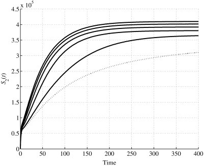
Time history of S₂(t) for values 0 ≤ u₁ ≤ u_1,0; the dashed line corresponds to u₁ = 0, the dotted line denotes the case u₁ = u_1,0.

Fig. 3.

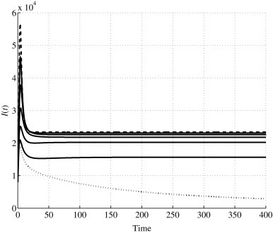
Time history of I(t) for values 0 ≤ u₁ ≤ u_1,0; the dashed line corresponds to u₁ = 0, the dotted line denotes the case u₁ = u_1,0.

Fig. 4.

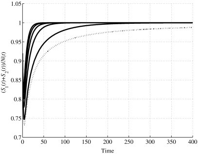
Time evolution of the relative number of healthy individuals S₁(t) + S₂(t) w.r.t. the total population for values 0 ≤ u₁ ≤ u_1,0; the dashed line corresponds to u₁ = 0, the dotted line denotes the case u₁ = u_1,0.

Fig. 5.

Time history of S₁(t) for values u₁ ≥ u_1,0.

Fig. 6.

Time history of S₂(t) for values u₁ ≥ u_1,0.

Fig. 7.

Time history of I(t) for values u₁ ≥ u_1,0.

Fig. 8.

Time evolution of the relative number of healthy individuals S₁(t) + S₂(t) w.r.t. the total population for values u₁ ≥ u_1,0.

For the first set, the values $u_1\in \left[0,0.1,\mathrm{0.20.30.4},0.5,u_{1,0}\right]$ are considered. In Fig. 1, Fig. 2, Fig. 3, Fig. 4, the dashed line denotes the evolutions for u ₁ = 0, while the dotted line represents the behaviors when u ₁ = u _1,0. The five solid lines are associated with the intermediate values: they show a behavior that uniformly goes from the uncontrolled one, dashed line, to the bifurcation value for the control, dotted line. Such a variation increases for S ₁(t) and S ₂(t), while it decreases for I(t). This means that as u ₁ increases, the parts of the population in S ₁(t) and S ₂(t), after an initial decrement, increases as well, showing, at each time, greater numbers for greater control amplitude and reaching, at steady state, greater numbers. Correspondingly, the infected population in I(t) evolves following smaller values at each time, the steady-state value decreases as u ₁ increases, till assuming zero as asymptotic value when u ₁ is equal to the bifurcation value. The overall effect is the increment in the fraction of healthy population, depicted in Fig. 4, reaching the full health condition as u ₁ → u _1,0.

In the second set, the values $u_1\in \left[u_{1,0},0.6,0.7,0.8,0.9,1\right]$ are considered. In this case also, in Fig. 5, Fig. 6, Fig. 7, Fig. 8, the dotted line represents the behavior when u ₁ = u _1,0. As previously proved, for u ₁ > u _1,0 the system has only one equilibrium point, the first one, and it is locally asymptotically stable. Then, according to the expression (27), the behavior of the state variable S ₁(t), for its steady-state value, decreases as u ₁ increases, and for the higher value simulated, u ₁ = 1, it reaches the value of 9.0164 × 10⁴. At the same time, S ₂ increases, as shown in Fig. 6; for u ₁ = 1, its steady-state value is 4.0984 × 10⁵, as expression (27) gives. The time history of I(t), depicted in Fig. 7, shows a faster convergence to zero as u ₁ increases, always having zero as steady-state value, according to Eq. (27). Then, all the population tends to be healthy, as shown in Fig. 8.

For the study of local stability of ${\xi }_2^e(u_1)$ an analogous analysis must be performed, starting with the evaluation of Eq. (19) in such an equilibrium point. The result is the block triangular matrix

(30)

with

$$\begin{array}{ll}\hfill A_2^{11}(u_1)& =\left(\begin{array}{ccc}-(d+u_1)-c\beta \frac{I^e}{N_c^e}\left(1-\frac{S_1^e}{N_c^e}\right)& \gamma +c\beta \frac{S_1^e}{N_c^e}\frac{I^e}{N_c^e}& -c\beta \frac{S_1^e}{N_c^e}\left(1-\frac{I^e}{N_c^e}\right)\\ u_1& -(\gamma +d)& 0\\ c\beta \frac{I^e}{N_c^e}\left(1-\frac{S_1^e}{N_c^e}\right)& -c\beta \frac{S_1^e}{N_c^e}\frac{I^e}{N_c^e}& -(d+\delta )+c\beta \frac{S_1^e}{N_c^e}\left(1-\frac{I^e}{N_c^e}\right)\end{array}\right)\hfill \end{array}$$ (31)

$$\begin{array}{ll}\hfill A_2^{21}& =\left(\begin{array}{ccc}\hfill 0\hfill & \hfill 0\hfill & \hfill \varepsilon \delta \hfill \\ \hfill 0\hfill & \hfill 0\hfill & \hfill (1-\varepsilon )\delta \hfill \end{array}\right)A_2^{22}=\left(\begin{array}{cc}\hfill -({\alpha }_1+d)\hfill & \hfill 0\hfill \\ \hfill {\alpha }_1\hfill & \hfill -(\alpha +d)\hfill \end{array}\right)\hfill \end{array}$$ (32)

After some computations, the characteristic polynomial of matrix (31) can be written as

$$\begin{array}{l}\hfill p(\lambda )={\lambda }^3+m_2{\lambda }^2+m_1\lambda +m_0\end{array}$$

with

$$\begin{array}{ll}\hfill m_2& =\left(c\beta -\delta +(\gamma +d)+\frac{\gamma -\delta }{\gamma +d}{u}_1\right)\hfill \\ \hfill m_1& =(c\beta -\delta )\left((\gamma +d)+\frac{(c\beta -(d+\delta ))(d+\delta )}{c\beta }\right)\hfill \\ \hfill & +\delta u_1-\frac{{(d+\delta )}^2(c\beta -\delta )}{c\beta (\gamma +d)}{u}_1\hfill \\ \hfill m_0& =-\frac{(d+\delta )(c\beta -(d+\delta ))(\gamma +d)(c\beta -\delta )}{c\beta }\hfill \\ \hfill & +\frac{d+\delta }{c\beta }\left(dc\beta +2\delta (c\beta -(d+\delta ))\right)u_1-\delta \frac{{(d+\delta )}^2}{c\beta (\gamma +d)}{u}_1^2\hfill \end{array}$$ (33)

The conditions for the local stability of the equilibrium point (17) are

$$\begin{array}{l}\hfill m_i>0,i=0,1,2\text{and}{m}_1{m}_2>m_0\end{array}$$ (34)

For the numerical case referred here, the equilibrium point is Eq. (28) and the Jacobian matrix (31) becomes

$$\begin{array}{l}\hfill A_2^{11}(u_1)=\left(\begin{array}{ccc}\hfill -0.7976+0.3745u_1\hfill & \hfill 0.5024-0.5345u_1\hfill & \hfill -0.1176-0.5345u_1\hfill \\ \hfill u_1\hfill & \hfill -0.2200\hfill & \hfill 0\hfill \\ \hfill 0.7776-1.3745u_1\hfill & \hfill -0.3024+0.5345u_1\hfill & \hfill -0.3024+0.5345u_1\hfill \end{array}\right)\end{array}$$ (35)

In Fig. 9 , the real part of the three eigenvalues of matrix (35) for values of u ₁ ∈ [0, 1] are reported. It can be observed that, for u ₁ < u _1,0 = 0.5657, highlighted in the figure with the vertical dotted line, the linearized dynamics is asymptotically stable, then the equilibrium point ${\xi }_2^e(u_1)$ (Eq. 17) exists as a second equilibrium point and is asymptotically stable (the endemic condition). Above that value, one eigenvalue becomes positive. The results of this analysis are that the equilibrium and the stability conditions of the dynamics (Eq. 1) can be affected by external inputs, u ₁ in this case, even leading to the loss of some stability properties.

Fig. 9.

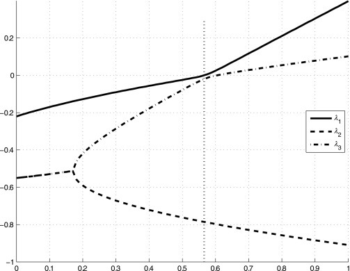
Real part of the eigenvalues of Eq. (35) for u₁ ∈ [0, 1] are reported. The vertical dotted line denotes u_1,0 = 0.5657, the bifurcation value.

In the following section, the same study is carried on for the input u ₂, aiming to show whether the influence of the input on the stability is present for the second input too.

5.2. Analysis of the case u₁(t) = u₃(t) = 0 and u₂(t) = u₂

The case of a constant input u ₂≠0 is now considered in Section 5.2. As in Section 5.1, first the equilibrium points are computed and then their stability properties are studied.

5.2.1. Equilibria computation for u₂≠0

In this case, to compute the new equilibria, the nonlinear system

$$\begin{array}{l}\hfill f(S_1^e,S_2^e,I^e,P^e,A^e)+g_2(S_1^e,S_2^e,I^e,P^e,A^e)u_2=0\end{array}$$ (36)

has to be solved. It is the same as Eq. (4), with the addition of g ₂(ξ(t))u ₂, with g ₂ as in Eq. (3). Performing the computations, the solution

$$\begin{array}{l}\hfill {\xi }_1^e(u_2)={\left(\begin{array}{ccccc}\hfill \frac{1}{d}\hfill & \hfill 0\hfill & \hfill 0\hfill & \hfill 0\hfill & \hfill 0\hfill \end{array}\right)}^{T}Q\end{array}$$ (37)

is obtained; it does not depend on u ₂ and it is the same as the unforced case ${\xi }_1^e$ in Eq. (5). Moreover, once $S_2^e=0$ is obtained, computations give also the expressions

$$\begin{array}{ll}\hfill & I^e=\frac{c\beta -(d+\delta )}{d+\delta }{S}_1^e-\frac{\psi u_2}{d+\delta }\hfill \end{array}$$ (38)

$$\begin{array}{ll}\hfill & c\beta (\delta -c\beta ){(S_1^e)}^2+\left(c\beta Q+\psi u_2(d+c\beta )\right)S_1^e-\psi Q{u}_2=0\hfill \end{array}$$ (39)

Note that if u ₂ = 0, from Eq. (38) one has the same condition on the uncontrolled case and, in fact, Eq. (39) reduces to a first-order one, yielding the same solution as in Eq. (5). If (δ − cβ) > 0, the two roots of Eq. (39) are real, one positive and one negative; then, one value for the equilibrium point can be obtained, the positive root, say $S_1^{e_0}(u_2)$. On the other hand, if (δ − cβ) < 0, both the solutions have positive real part. They are real, then they are equilibrium points, if and only if

$$\begin{array}{l}\hfill {\left(Qc\beta +\psi u_2(d+c\beta )\right)}^2>4c\beta Q\psi u_2|\delta -c\beta |\end{array}$$ (40)

If Eq. (40) is satisfied, two solutions $S_1^{e_1}(u_2)$ and $S_1^{e_2}(u_2)$ are obtained for Eq. (39). Then, for the first three components of the equilibrium points, three cases are possible, according to the values of the parameters and the input u ₂: (i) for δ − cβ > 0, one value for $S_1^e(u_2)$ is obtained, $S_1^{e_0}(u_2)$, solving Eq. (39) and taking the only positive solution; (ii) for δ − cβ < 0, if Eq. (40) holds, two solutions $S_1^{e_1}(u_2)$ and $S_1^{e_2}(u_2)$ are obtained solving Eq. (39); (iii) for δ − cβ < 0, if Eq. (40) does not hold, no admissible (real) solutions are obtained from Eq. (39). Consequently, the corresponding values for the equilibrium I ^e(u ₂) can be computed from Eq. (38) and denoted by $I^{e_i}(u_2)$, i = 0, 1, 2 correspondingly to the value $S_1^{e_i}(u_2)$, while $S_2^e(u_2)=0$ holds in any case. For the remaining two components P ^e(u ₂) and A ^e(u ₂) using Eq. (38), one has

$$\begin{array}{ll}\hfill P^{e_i}(u_2)& =\left(\frac{\varepsilon \delta }{{\alpha }_1+d}+\frac{\varphi \psi }{({\alpha }_1+d)\left(S_1^{e_i}(u_2)+I^{e_i}\right)}{u}_2\right)I^{e_i}\hfill \end{array}$$ (41)

$$\begin{array}{ll}\hfill A^{e_i}(u_2)& =(1-\varepsilon )\delta I^{e_i}(u_2)+{\alpha }_1{P}^{e_i}(u_2)+\frac{(1-\varphi )\psi I^{e_i}(u_2)}{(\alpha +d)\left(S_1^{e_i}(u_2)+I^{e_i}(u_2)\right)}{u}_2\hfill \end{array}$$ (42)

The equilibrium points ${\xi }_2^{e_i}(u_2)$ can then be written as

$$\begin{array}{l}\hfill {\xi }_2^{e_i}(u_2)={\left(\begin{array}{ccccc}\hfill S_1^{e_i}(u_2)\hfill & \hfill 0\hfill & \hfill I^{e_i}(u_2)\hfill & \hfill P^{e_i}(u_2)\hfill & \hfill A^{e_i}(u_2)\hfill \end{array}\right)}^T\end{array}$$ (43)

5.2.2. Stability analysis for the equilibrium ${\xi }_1^e(u_2)$

Once again, the study of local stability for the equilibrium points (37), (43) can be performed referring to their linear approximations. The study for ${\xi }_1^e(u_2)$ in Eq. (37) provides with the matrix

(44)

Then, in addition to the four constant negative eigenvalues λ ₁ = −d, λ ₂ = −(γ + d), λ ₃ = −(α ₁ + d), and λ ₄ = −(α + d), there is one eigenvalue which is the function of the input u ₂, λ ₅ = cβ − (d + δ) − ψu ₂. If cβ − (d + δ) < 0, the same as Eq. (9), then λ ₅ < 0 ∀u ₂ ≥ 0. On the other hand, if condition (9) is not verified for the uncontrolled system, there exists a value $u_{2,0}=\frac{c\beta -(d+\delta )}{\psi }$ such that λ ₅ < 0 ∀u ₂ > u _{2, 0}. This means that a system, for which the parameters are such that the equilibrium ${\xi }_1^e$ is unstable, under the action of an input u ₂ can become stable. Once again, the effect of a control input, in this case, u ₂, affects the stability properties of a system (1).

5.2.3. Stability analysis for the equilibrium ${\xi }_2^{e_i}(u_2)$

On the basis of the discussion in Section 5.2.1, the existence, and hence the stability, of the equilibrium points ${\xi }_2^{e_i}(u_2)$ (Eq. 43), is highly dependent on the values of the system parameters. Thus, an analytical study of their stability involves long and complicated expressions, not useful for qualitative discussions. To show the effects of an input u ₂ on the existence and the stability of the points (43), a numerical analysis is performed, making use of the values introduced in Table 1 .

Table 1.

Numerical values of the model parameters

Parameter	Value		Parameter	Value
d	0.02		c	10
β	0.15		γ	0.2
δ	0.4		ψ	100,000
ɛ	0.6		α1	0.5
ϕ	0.95		α	1
Q	104

Numerical simulations are performed for u ₁ = u ₃ = 0 and for values of u ₂ in the set u ₂ ∈{0, 0.2, 0.4, 0.6, 0.8, 1}. Some of the results are reported in Fig. 10, Fig. 11, Fig. 12, Fig. 13, Fig. 14, Fig. 15, Fig. 16, Fig. 17 . In all the figures, the case u ₂ = 0, the uncontrolled case, is depicted by the dashed line, for comparative purpose with the other increasing values. Figs. 10 and 11 show the time histories of the two state components S ₁(t) and I(t), for different input values. Although monotonical increment in the individuals S ₁(t) as u ₂ increases is expected, as well as the corresponding decrement in the infected subjects I(t), there are two interesting results which the figures show. The first is the appearance of the oscillatory behavior which is related to the amplitude of the input u ₂. This kind of time evolution is well evidenced referring to Fig. 14, where the trajectories in the plane I(t) + P(t) + A(t) versus S ₁(t) + S ₂(t) is plotted: the spiral trajectory while converging to the equilibrium point is clearly visible. This means that, under input u ₂ ≠ 0, there are time instants in which the number of the infected individuals I(t) can seem greater than expected, but it is related to the transient behavior only. The second result puts in evidence from the numerical simulations is that the number of diagnosed infected individuals P(t) and A(t) do not decrease as I(t) decreases. This is due to the fact that the action of the control u ₂ aims at increasing the number of diagnoses, so that while I(t) decreases, people moves to P(t) (Fig. 12) and A(t) (Fig. 13). The overall effects on the total population is shown in Fig. 15, where its increment is clear. While the total population increases, the fraction of healthy people S ₁(t) + S ₂(t) with respect to the total population strongly increases, as reported in Fig. 16 and, at the same time, the fraction of diagnosed patients P(t) + A(t) significantly decreases (Fig. 17).

Fig. 10.

Time history of S₁(t) for u₂ ∈{0, 0.2, 0.4, 0.6, 0.8, 1}. The dashed line depicts the case u₂ = 0, the behaviors change monotonically with u₂.

Fig. 11.

Time history of I(t) for u₂ ∈{0, 0.2, 0.4, 0.6, 0.8, 1}. The dashed line depicts the case u₂ = 0, the behaviors change monotonically with u₂.

Fig. 12.

Time history of P(t) for u₂ ∈{0, 0.2, 0.4, 0.6, 0.8, 1}. The dashed line depicts the case u₂ = 0, the behaviors change monotonically with u₂.

Fig. 13.

Time history of A(t) for u₂ ∈{0, 0.2, 0.4, 0.6, 0.8, 1}. The dashed line depicts the case u₂ = 0, the behaviors change monotonically with u₂.

Fig. 14.

Time history of A(t) for u₂ ∈{0, 0.2, 0.4, 0.6, 0.8, 1}. The dashed line depicts the case u₂ = 0, the behaviors change monotonically with u₂.

Fig. 15.

Time evolution of the total population for u₂ ∈{0, 0.2, 0.4, 0.6, 0.8, 1}. The dashed line depicts the case u₂ = 0, the behaviors change monotonically with u₂.

Fig. 16.

Time evolution of the healthy individuals S₁(t) + S₂(t) with respect to the total population for u₂ ∈{0, 0.2, 0.4, 0.6, 0.8, 1}. The dashed line depicts the case u₂ = 0, the behaviors change monotonically with u₂.

Fig. 17.

Time evolution of the diagnosed patients P(t) + A(t) with respect to the total population for u₂ ∈{0, 0.2, 0.4, 0.6, 0.8, 1}. The dashed line depicts the case u₂ = 0, the behaviors change monotonically with u₂.

6. The interactions between populations

The study of the effects on a population of the interactions with different groups can be performed by modeling the whole population as the aggregate of each one and introducing terms in the dynamics which take into account the possible interconnections. For the dynamics (1) considered in Section 3, this would bring to a 5N-dimensional system, N being the number of groups considered. A characterization of the entire population could then possibly increase the complexity of the whole expression.

Taking one of the N population and considering all the interactions with the remaining N − 1 ones by means of global averaged terms, the mathematical model can be strongly simplified introducing changes in Eq. (1) which can take into account the combined effects of the external interactions. Clearly, many details are lost since some contributions are averaged, but a useful preliminary analysis can be performed. On the basis of the results obtained for the single group model in previous sections, the evidence and the effects of the changes introduced in a population by the interactions with external world can be obtained once such interactions are suitably modeled as additional inputs and/or changes in the parameter values. Concerning the additional inputs, these can be assumed as the sum of the effects of migration, positive and negative, between the group under investigation with respect to all the other ones. Such effects can be modeled as constant fluxes, which introduce additive constant terms in the dynamics, or can be supposed to be driven by some characteristic of the group behavior, such as the public health level.

Migrations can also affect the value of some parameters, representing changes in the behavior of some individuals consequent to some cultural modifications. For examples, c and β for the number of the contagious interactions depend also on the cultural and educational facts, γ for the attitude of ignoring the dangerous effects of some kind of relationships, and so on.

In the present study, the assumption that the health status of a population can be an indicator of its attractiveness, being related to the richness, the higher social level, and so on, the changes introduced in model (1) to take into account the interactions with other groups are represented by the introduction of additional terms of the form f _i(S ₁, S ₂, I, P, A), i = 1 for S ₁, i = 2 for S ₂, and i = 3 for I, assuming that known infected individuals P and A are not allowed to migrate. Then, Eq. (1) becomes

$$\begin{array}{ll}\hfill & {\dot{S}}_1(t)=Q-d{S}_1(t)-\frac{c\beta S_1(t)I(t)}{N_c(t)}+\gamma S_2(t)-S_1(t)u_1(t)+f_1(S_1,S_2,I,P,A)\hfill \end{array}$$ (45a)

$$\begin{array}{ll}\hfill & {\dot{S}}_2(t)=-(\gamma +d)S_2(t)+S_1(t)u_1(t)+f_2(S_1,S_2,I,P,A)\hfill \end{array}$$ (45b)

$$\begin{array}{ll}\hfill & İ(t)=\frac{c\beta S_1(t)I(t)}{N_c(t)}-(d+\delta )I(t)-\psi \frac{I(t)}{N_c(t)}{u}_2(t)+f_3(S_1,S_2,I,P,A)\hfill \end{array}$$ (45c)

$$\begin{array}{ll}\hfill & \dot{P}(t)=\varepsilon \delta I(t)-({\alpha }_1+d)P(t)+\varphi \psi \frac{I(t)}{N_c(t)}{u}_2(t)+P(t)u_3(t)\hfill \end{array}$$ (45d)

$$\begin{array}{ll}\hfill & \dot{A}(t)=(1-\varepsilon )\delta I(t)+{\alpha }_{1}P(t)-(\alpha +d)A(t)+(1-\varphi )\psi \frac{I(t)}{N_c(t)}{u}_2(t)-P(t)u_3(t)\hfill \end{array}$$ (45e)

Some choices for f _i(S ₁, S ₂, I, P, A), under the assumption previously mentioned, can be, for example, proportional to $\frac{S_1+S_2+I}{S_1+S_2+I+P+A}$, meaning that the more the group is healthy, the more it is attractive, or proportional to $-\frac{P+A}{S_1+S_2+I+P+A}$, meaning that the higher is the number of the infectious patients, the more it is repulsive. Simplified versions can be considered neglecting the normalizing denominators. In following section, the choice

$$\begin{array}{l}\hfill f_i(S_1,S_2,I,P,A)=m_i\frac{S_1+S_2+I}{N}-n_i\frac{P+A}{N}\end{array}$$ (46)

is adopted, i = 1, 2, 3, where N = S ₁ + S ₂ + I + P + A.

This corresponds to the introduction, in the most general formulation, of both an immigration term

$$\begin{array}{l}\hfill m_i\frac{S_1+S_2+I}{S_1+S_2+I+P+A}\end{array}$$ (47)

and an emigration one

$$\begin{array}{l}\hfill n_i\frac{P+A}{S_1+S_2+I+P+A}\end{array}$$ (48)

to each of the involved dynamics, that is, for S ₁, S ₂, and I. In this case, the effects of the migration fluxes vary according to the values of the six parameters m _i and n _i, for i = 1, 2, 3.

6.1. Equilibria under external interactions

In this section, the effects on the equilibrium conditions of the external interactions just introduced are studied. A full analysis should be performed to study the effect of the changes of the new six parameters on the dynamics behavior. In order to better identify the relationships between each contribution and the corresponding effect, the analysis is performed isolating some particular fluxes. In particular, two cases are separately addressed. The first supposes that the contribution of the immigration/emigration flux acts on the susceptible group S ₁ only, aiming at analyzing what may happen when the number of uninfected people changes due to migrations. The second one is, in some sense, the dual case: the effects of the migration are evaluated under the hypothesis that all the flux is concentrated on the infected but not diagnosed individuals I. With respect to the model introduced here for the interactions (45), in the terms (46), m ₂ = m ₃ = n ₂ = n ₃ = 0 are chosen for the first case investigated, while m ₁ = m ₃ = n ₁ = n ₃ = 0 are assumed for the second case.

Equilibrium points and their stability are first analyzed, in order to characterize the dynamical properties and to be able to compare the results with the isolated group case mentioned in Section 3.

6.1.1. Equilibrium points and stability properties for the case of healthy population migration

Under the hypothesis previously described, in this case the equilibrium points are computed solving the nonlinear system

$$\begin{array}{ll}\hfill Q-d{S}_1^e-\frac{c\beta S_1^e{I}^e}{N_c^e}+\gamma S_2^e+m_1\frac{S_1^e+S_2^e+I^e}{N^e}-n_1\frac{P^e+A^e}{N^e}& =0\hfill \end{array}$$ (49)

$$\begin{array}{ll}\hfill -(\gamma +d)S_2^e& =0\hfill \end{array}$$ (50)

$$\begin{array}{ll}\hfill \frac{c\beta S_1^e{I}^e}{N_c^e}-(d+\delta )I^e& =0\hfill \end{array}$$ (51)

$$\begin{array}{ll}\hfill \varepsilon \delta I^e-({\alpha }_1+d)P^e& =0\hfill \end{array}$$ (52)

$$\begin{array}{ll}\hfill (1-\varepsilon )\delta I^e+{\alpha }_1{P}^e-(\alpha +d)A^e& =0\hfill \end{array}$$ (53)

One solution is given by

$$\begin{array}{l}\hfill {\xi }_1^e(m_1,n_1)={\left(\begin{array}{ccccc}\hfill \frac{Q+m_1}{d}\hfill & \hfill 0\hfill & \hfill 0\hfill & \hfill 0\hfill & \hfill 0\hfill \end{array}\right)}^T\end{array}$$ (54)

Then, setting

$$\begin{array}{l}\hfill P^e+A^e=\frac{\delta }{{\alpha }_1+d}\left(\frac{\varepsilon \alpha +{\alpha }_1+d}{\alpha +d}\right)I^e=\pi I^e\end{array}$$ (55)

and performing some computations, the second solution

$$\begin{array}{l}\hfill {\xi }_2^e(m_1,n_1)=\left(\begin{array}{c}\hfill \frac{Q}{c\beta -\delta }+\frac{m_{1}c\beta -n_1\pi (c\beta -(d+\delta ))}{(c\beta (1+\pi )-\pi (d+\delta ))(c\beta -\delta )}\hfill \\ \hfill 0\hfill \\ \hfill \frac{c\beta -(d+\delta )}{d+\delta }\left(\frac{Q}{c\beta -\delta }+\frac{m_{1}c\beta -n_1\pi (c\beta -(d+\delta ))}{(c\beta (1+\pi )-\pi (d+\delta ))(c\beta -\delta )}\right)\hfill \\ \hfill \frac{\varepsilon \delta }{{\alpha }_1+d}\frac{c\beta -(d+\delta )}{d+\delta }\left(\frac{Q}{c\beta -\delta }+\frac{m_{1}c\beta -n_1\pi (c\beta -(d+\delta ))}{(c\beta (1+\pi )-\pi (d+\delta ))(c\beta -\delta )}\right)\hfill \\ \hfill \frac{\delta \left({\alpha }_1+d(1-\varepsilon )\right)}{(\alpha +d)({\alpha }_1+d)}\frac{c\beta -(d+\delta )}{d+\delta }\left(\frac{Q}{c\beta -\delta }+\frac{m_{1}c\beta -n_1\pi (c\beta -(d+\delta ))}{(c\beta (1+\pi )-\pi (d+\delta ))(c\beta -\delta )}\right)\hfill \end{array}\right)\end{array}$$ (56)

is obtained. The existence of this solution depends on the coefficients m ₁ and n ₁, since it must be verified that $S_1^e\ge 0$. However, once the condition on $S_1^e$ is satisfied, from I ^e ≥ 0 the condition cβ − (d + δ) ≥ 0 must hold. This is the same as Eq. (6) for ${\xi }_2^e$ in Section 4.1. Expression (56) can be simplified writing

$$\begin{array}{l}\hfill {\xi }_2^e(m_1,n_1)=\left(\begin{array}{c}\hfill C_0+C_m{m}_1-C_n{n}_1\hfill \\ \hfill 0\hfill \\ \hfill K_I\left(C_0+C_m{m}_1-C_n{n}_1\right)\hfill \\ \hfill K_P\left(C_0+C_m{m}_1-C_n{n}_1\right)\hfill \\ \hfill K_A\left(C_0+C_m{m}_1-C_n{n}_1\right)\hfill \end{array}\right)\end{array}$$ (57)

once the following coefficients are defined:

$$\begin{array}{ll}\hfill C_0& =\frac{Q}{c\beta -\delta }\hfill \end{array}$$ (58)

$$\begin{array}{ll}\hfill C_m& =\frac{c\beta }{(c\beta (1+\pi )-\pi (d+\delta ))(c\beta -\delta )}\hfill \end{array}$$ (59)

$$\begin{array}{ll}\hfill C_n& =\frac{\pi (c\beta -(d+\delta ))}{(c\beta (1+\pi )-\pi (d+\delta ))(c\beta -\delta )}\hfill \end{array}$$ (60)

$$\begin{array}{ll}\hfill K_I& =\frac{c\beta -(d+\delta )}{d+\delta }\hfill \end{array}$$ (61)

$$\begin{array}{ll}\hfill K_P& =\frac{\varepsilon \delta }{{\alpha }_1+d}{K}_I\hfill \end{array}$$ (62)

$$\begin{array}{ll}\hfill K_A& =\frac{\delta \left({\alpha }_1+d(1-\varepsilon )\right)}{(\alpha +d)({\alpha }_1+d)}{K}_I\hfill \end{array}$$ (63)

The structure of expression (57) shows that the equilibrium point linearly change w.r.t. both m ₁ and n ₁.

The study of the stability characteristics for the two equilibrium points is performed, once again, analyzing the stability of the linearized dynamics in the neighborhood of the equilibria. For the first point ${\xi }_1^e(m_1,n_1)$, the Jacobian matrix computed in the equilibrium point is the same as for the isolated unforced case ${\xi }_1^e$ in Eq. (5). Its expression is given in Eq. (7) and the same stability conditions can be obtained: the equilibrium point ${\xi }_1^e(m_1,n_1)$ is locally asymptotically stable under condition (9). For the second equilibrium point ${\xi }_2^e(m_1,n_1)$ in Eq. (57), the dynamical matrix of the linear approximation has the structure

(64)

with $A_2^{22}(m_1,n_1)$ equal to the one in Eq. (12) for the isolated unforced case, for which the two eigenvalues, λ ₄ = −(α ₁ + d) and λ ₅ = −(α + d), are real negative. Then, for the stability conditions, matrix

$$\begin{array}{l}\hfill A_2^{11}(m_1,n_1)=\left(\begin{array}{ccc}\hfill -d-c\beta \frac{K_I^2}{{(1+K_I)}^2}\hfill & \hfill \gamma +c\beta \frac{K_I}{{(1+K_I)}^2}\hfill & \hfill -c\beta \frac{1}{{(1+K_I)}^2}\hfill \\ \hfill 0\hfill & \hfill -(\gamma +d)\hfill & \hfill 0\hfill \\ \hfill c\beta \frac{K_I^2}{{(1+K_I)}^2}\hfill & \hfill -c\beta \frac{K_I}{{(1+K_I)}^2}\hfill & \hfill c\beta \frac{1}{{(1+K_I)}^2}-(d+\delta )\hfill & \hfill \hfill \\ \hfill \hfill \end{array}\right)\end{array}$$ (65)

must be analyzed. It is interesting to note that it does not depend on the coefficients m ₁ or n ₁; then, the same holds for the stability of the equilibrium points obtained by varying such coefficients. One of the eigenvalues of Eq. (65), λ ₃ = −(γ + d) < 0, is evident from the structure. The other two can be computed as the roots of the polynomial equation

$$\begin{array}{l}\hfill {\lambda }^2+\left(d+(d+\delta )-c\beta \frac{1-K_I^2}{{(1+K_I)}^2}\right)\lambda +\left(d(d+\delta )+c\beta \frac{(d+\delta )K_I^2-d}{{(1+K_I)}^2}\right)\end{array}$$ (66)

or, by replacing the full expression for K _I and performing all the simplifications,

$$\begin{array}{l}\hfill {\lambda }^2+(c\beta -\delta )\lambda +(d+\delta )(c\beta -\delta )\frac{c\beta -(d+\delta )}{c\beta }=0\end{array}$$ (67)

which is the same as Eq. (13). On the basis of the discussion in Section 4.2, it is possible to conclude that the condition for the local asymptotic stability for ${\xi }_2^e(m_1,n_1)$ does not depend on m ₁ and n ₁ and it is the same as given in Eq. (14). Moreover, the same relationships between existence and stability of the two equilibrium points, as in Section 4.2 for ${\xi }_1^e$ and ${\xi }_2^e$, hold.

6.1.2. Equilibrium points and stability properties for the case of infected population migration

Following the same procedure as in the previous cases, the equilibrium points are computed solving the nonlinear system

$$\begin{array}{ll}\hfill Q-d{S}_1^e-\frac{c\beta S_1^e{I}^e}{N_c^e}+\gamma S_2^e& =0\hfill \end{array}$$ (68)

$$\begin{array}{ll}\hfill -(\gamma +d)S_2^e& =0\hfill \end{array}$$ (69)

$$\begin{array}{ll}\hfill \frac{c\beta S_1^e{I}^e}{N_c^e}-(d+\delta )I^e+m_3\frac{S_1^e+S_2^e+I^e}{N^e}-n_3\frac{P^e+A^e}{N^e}& =0\hfill \end{array}$$ (70)

$$\begin{array}{ll}\hfill \varepsilon \delta I^e-({\alpha }_1+d)P^e& =0\hfill \end{array}$$ (71)

$$\begin{array}{ll}\hfill (1-\varepsilon )\delta I^e+{\alpha }_1{P}^e-(\alpha +d)A^e& =0\hfill \end{array}$$ (72)

From Eq. (69) $S_2^e=0$ is immediately obtained. Once $N_c^e=S_1^e+I^e$ and $N^e=S_1^e+(1+\pi )I^e=N_c^e+\pi I^e$ are introduced, the system to be solved can be reduced to Eqs. (68), (70), and rewritten as

$$\begin{array}{ll}\hfill Q-d{S}_1^e-\frac{c\beta S_1^e{I}^e}{S_1^e+I^e}& =0\hfill \end{array}$$ (73)

$$\begin{array}{ll}\hfill \frac{c\beta S_1^e{I}^e}{S_1^e+I^e}-(d+\delta )I^e+m_3\frac{S_1^e+I^e}{S_1^e+(1+\pi )I^e}-n_3\frac{\pi I^e}{S_1^e+(1+\pi )I^e}& =0\hfill \end{array}$$ (74)

From Eq. (73), one can write

$$\begin{array}{l}\hfill I^e=\frac{(d{S}_1^e-Q)}{Q-(c\beta +d)S_1^e}{S}_1^e\end{array}$$ (75)

while, for $S_1^e$, after computations one gets the polynomial equation

$$\begin{array}{l}\hfill a_3{\left(S_1^e\right)}^3+a_2{\left(S_1^e\right)}^2+a_1{S}_1^e+a_0=0\end{array}$$ (76)

whose coefficients are as follows:

$$\begin{array}{ll}\hfill a_3& =d(c\beta -\delta )(c\beta -\pi d)\hfill \\ \hfill a_2& =2\pi Qd(c\beta -\delta )-(c\beta +d)(c\beta (Q+m_3)+\pi d{n}_3)+Qc\beta \delta +\pi Q{d}^2\hfill \\ \hfill a_1& =c\beta Q\left(Q(1-\pi )+m_3+\pi n_3\right)+\pi Q^2\delta -2\pi Qd\left(Q-n_3\right)\hfill \\ \hfill a_0& =\pi Q^2\left(Q-n_3\right)\hfill \end{array}$$ (77)

The feasible solutions correspond to the real positive roots of polynomial (76). Conditions should be given for the coefficients to characterize the roots in order to have admissible solutions but they are not easy to be written and their analysis requires a numerical evaluation of such conditions. Hence, from now on, the numerical values reported in Table 1 are used to show a possible behavior and also for comparative purpose with all the results and the discussions given in Section 5.

With the parameters presented in Table 1, coefficients (77) assume the following expression depending on the two parameters m ₃ and n ₃:

$$\begin{array}{ll}\hfill a_3& =0.0326\hfill \end{array}$$ (78)

$$\begin{array}{ll}\hfill a_2& =-2.2800m_3-0.0257n_3-1.6425\times 10^4\hfill \end{array}$$ (79)

$$\begin{array}{ll}\hfill a_1& =15,000m_3+1.3008\times 10^4{n}_3+5.3710\times 10^7\hfill \end{array}$$ (80)

$$\begin{array}{ll}\hfill a_0& =-8.4465\times 10^7{n}_3+8.4465\times 10^{11}\hfill \end{array}$$ (81)

The three solutions of Eq. (76) are computed for different values of m ₃ ∈ [0, 5 × 10⁴] and n ₃ ∈ [0, 5 × 10⁴]. In Fig. 18, Fig. 19, Fig. 20 , the variations of such solutions with respect to m ₃ are reported, keeping n ₃ = 0, while Fig. 21, Fig. 22, Fig. 23 depict how the solutions vary according to different values of n ₃ with m ₃ = 0. In each figure, the solid line represents the real part of the solution and the dashed line denotes the imaginary part, so that it is easy to reject the solutions which are not consistent with the real condition of the state variables. In all the six figures, it can be observed that the values of the equilibrium components $S_1^e$ and I ^e are all real. Moreover, in order to be admissible values, the components of the state must be nonnegative. In this case, for the range of values for the parameters m ₃ and n ₃, it can be seen that keeping n ₃ = 0, the three roots $S_1^e$ of the polynomial (76) are real, two positive, Figs. 18 and 19, and one negative, Fig. 20, for all the values given to m ₃ ∈ [0, 5 × 10⁴]. The corresponding values for the equilibrium I ^e are negative for the first solution in Fig. 18 and positive for the remaining two cases, Figs. 19 and 20. While for m ₃ = n ₃ = 0 the first and second solutions are admissible, as m ₃ increases, only the second is a feasible solution; in this case, only one equilibrium point exists and its components $S_1^e$ and I ^e are given in Fig. 19 for each value of m ₃ in the range considered.

Fig. 18.

Values of the first solution $S_1^e$ in Eq. (76) and I^e in Eq. (75) for m₃ ∈ [0, 5 × 10⁴].

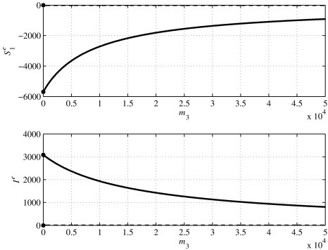
Fig. 19.

Values of the second solution $S_1^e$ in Eq. (76) and I^e in Eq. (75) for m₃ ∈ [0, 5 × 10⁴].

Fig. 20.

Values of the third solution $S_1^e$ in Eq. (76) and I^e in Eq. (75) for m₃ ∈ [0, 5 × 10⁴].

Fig. 21.

Values of the first solution $S_1^e$ in Eq. (76) and I^e in Eq. (75) for n₃ ∈ [0, 5 × 10⁴].

Fig. 22.

Values of the second solution $S_1^e$ in Eq. (76) and I^e in Eq. (75) for n₃ ∈ [0, 5 × 10⁴].

Fig. 23.

Values of the third solution $S_1^e$ in Eq. (76) and I^e in Eq. (75) for n₃ ∈ [0, 5 × 10⁴].

On the other hand, varying n ₃ while m ₃ = 0, the first solution, depicted in Fig. 21, shows that n ₃ does not influence one of the equilibrium point of the noninteracting case, defined in Section 4.1 as ${\xi }_1^e$. Also the second solution, plotted in Fig. 22, is admissible, since both $S_1^e$ and I ^e are positive for all the values considered for n ₃. On the contrary, the third solution cannot be assumed as an equilibrium point, because when $S_1^e$ is positive, I ^e is negative. Moreover, the value $S_1^e=0$ is never acceptable since it does not satisfy Eq. (73).

A stability analysis for the equilibrium points just computed is performed necessarily on the numerical case addressed till now. The Jacobian matrix (19) $J_f(\xi )=\frac{\partial f}{\partial \xi }$ must be computed and then evaluated at each equilibrium point. Since the structure of the system is the same as in Eq. (1) with the additional term

$$\begin{array}{l}\hfill m_3\frac{S_1+S_2+I}{N}-n_3\frac{P+A}{N}\end{array}$$ (82)

in the dynamics of the infected subjects I, expression (19) for the present case is the same as for Eq. (1) except for the third row depending on f ₃, in which the elements in Eq. (82) must be considered. What is then obtained is

$$\begin{array}{ll}\hfill \frac{\partial f_1}{\partial S_1}& =-d-\frac{c\beta I}{N_c}+\frac{c\beta S_{1}I}{N_c^2},\frac{\partial f_1}{\partial S_2}=\gamma +\frac{c\beta S_{1}I}{N_c^2}\hfill \end{array}$$ (83)

$$\begin{array}{ll}\hfill \frac{\partial f_1}{\partial I}& =-\frac{c\beta S_1}{N_c}+\frac{c\beta S_{1}I}{N_c^2},\frac{\partial f_2}{\partial S_2}=-(\gamma +d)\hfill \end{array}$$ (84)

$$\begin{array}{ll}\hfill \frac{\partial f_4}{\partial I}& =\varepsilon \delta ,\frac{\partial f_4}{\partial P}=-({\alpha }_1+d)\hfill \end{array}$$ (85)

$$\begin{array}{ll}\hfill \frac{\partial f_5}{\partial I}& =(1-\varepsilon )\delta ,\frac{\partial f_5}{\partial P}={\alpha }_1,\frac{\partial f_5}{\partial A}=-(\alpha +d)\hfill \end{array}$$ (86)

as for the isolated case, while for the third row one has

$$\begin{array}{ll}\hfill \frac{\partial f_3}{\partial S_1}& =\frac{c\beta I}{N_c}-\frac{c\beta S_{1}I}{N_c^2}+\frac{(m_3+n_3)(P+A)}{N^2}\hfill \end{array}$$ (87)

$$\begin{array}{ll}\hfill \frac{\partial f_3}{\partial S_2}& =-\frac{c\beta S_{1}I}{N_c^2}+\frac{(m_3+n_3)(P+A)}{N^2}\hfill \end{array}$$ (88)

$$\begin{array}{ll}\hfill \frac{\partial f_3}{\partial I}& =-(d+\delta )+\frac{c\beta S_1}{N_c}-\frac{c\beta S_{1}I}{N_c^2}+\frac{(m_3+n_3)(P+A)}{N^2}\hfill \end{array}$$ (89)

$$\begin{array}{ll}\hfill \frac{\partial f_3}{\partial P}& =-\frac{(m_3+n_3)(S_1+S_2+I)}{N^2}\hfill \end{array}$$ (90)

$$\begin{array}{ll}\hfill \frac{\partial f_3}{\partial A}& =-\frac{(m_3+n_3)(S_1+S_2+I)}{N^2}\hfill \end{array}$$ (91)

The corresponding Jacobian matrix is computed for each of the admissible equilibrium points obtained in Section 6.1. Then, for the case n ₃ = 0, only one solution is considered, whose value changes with m ₃ (Fig. 19). For each value of m ₃, one equilibrium point is obtained as well as one corresponding Jacobian matrix. For each of them five eigenvalues are computed and are plotted in Fig. 24 . It can be noted that all the five eigenvalues, three real and one conjugate complex pair, have their real part negative until m ₃ = 2.285 × 10⁴, marked with the dotted vertical line. Above that value, one eigenvalue becomes positive and the local stability is lost.

Fig. 24.

Real part of the five eigenvalues of the Jacobian matrix computed in the first solution for n₃ = 0 and m₃ ∈ [0, 5 × 10⁴]. The dotted line denotes the real part of a couple of conjugate complex roots.

The same computations are performed for the two admissible equilibrium points reported in Figs. 21 and 22. The eigenvalues of the Jacobian matrix which locally approximates the nonlinear dynamics in a neighborhood of the n ₃-dependent first equilibrium point are reported in Fig. 25 , where it is possible to see that for the range considered for n ₃, one root is always positive and so the equilibrium point is unstable. On the contrary, for the second equilibrium point, the one in Fig. 22, the situation is equivalent to the case in Fig. 24: three real eigenvalues and one conjugate complex pair, whose real parts are depicted in Fig. 26 , solid line for the real roots, dashed line for the complex ones. They are all negative for n ₃ < 8.4 × 10⁵, so yielding to local asymptotic stability of the equilibrium points; for values n ₃ > 8.4 × 10⁵ stability condition is no more satisfied.

Fig. 25.

Real part of the five eigenvalues of the Jacobian matrix computed in the first solution for m₃ = 0 and n₃ ∈ [0, 5 × 10⁴].

Fig. 26.

Real part of the five eigenvalues of the Jacobian matrix computed in the second solution for n₃ = 0 and m₃ ∈ [0, 5 × 10⁴]. The dotted line denotes the real part of a couple of conjugate complex roots.

7. The effects of migration parameters on the individuals evolutions

This section is devoted to report some behavior of the system for different values of the coefficients m ₁, n ₁, m ₃, and n ₃, according to the stability results discussed in Section 6. The numerical values of the system parameters are, obviously, the ones illustrated in Table 1; the initial conditions for all the simulations have been chosen as S ₁(0) = 92, 000, I(0) = 8000, S ₂(0) = P(0) = A(0) = 0, aiming at modeling a population in which, initially, the epidemic is not known but some infected individuals are already present.

The first case reported refers to the time evolution of the system where m ₁ varies while n ₁ = m ₃ = n ₃ = 0. The results are reported in Fig. 27, Fig. 28, Fig. 29, Fig. 30, Fig. 31 . In particular, Fig. 27 depicts the evolution of the number of unwise healthy population S ₁(t) when m ₁ changes and Fig. 28 reports the same cases for m ₁, starting from zero (corresponding to the dashed lines) and increasing its value. The evolution of S ₂(t) is not reported because for the initial condition chosen it is constant and equal to zero. Also the time histories of P(t) and A(t) are omitted since they have the same shape of I(t). The obvious result that can be evidenced from Fig. 27 is that the number of healthy people increases as m ₁ grows; unfortunately, this increment makes the infected individuals I(t) grow too. However, a very interesting behavior of the system can be observed once the evolution of the fraction of diagnosed infected patients P(t) + A(t) w.r.t. the total population is determined, varying m ₁, as reported in Fig. 29. From these plots it can be seen that, under the hypothesis of an immigration of healthy people driven by the health of the total population, the different values of m ₁ affects the transient behavior only, reaching, for all m ₁, the same steady-state value. The same result can be observed in Fig. 30, where the fraction of the healthy population S ₁(t) + S ₂(t) w.r.t. the total one is reported: also in this case, the steady-state value is the same. Thus, it is possible to conclude that, for the model considered, an immigration of healthy individuals makes the population grow, as evidenced in Fig. 31; each of the classes grows (Figs. 27 and 28) but the fraction of healthy population as well as the fraction of infected one tends to remain unchanged even if the rate of immigration (m ₁) increases.

Fig. 27.

Time history of S₁(t) for different values of m₁. The dotted line corresponds to m₁ = 0; values increases according to m₁.

Fig. 28.

Time history of I(t) for different values of m₁. The dotted line corresponds to m₁ = 0; values increases according to m₁.

Fig. 29.

Time evolution of the relative number of diagnosed patients P(t) + A(t) w.r.t. the total population for different values of m₁. The dotted line corresponds to m₁ = 0.

Fig. 30.

Time evolution of the relative number of healthy individuals S₁(t) + S₂(t) w.r.t. the total population for different values of m₁. The dotted line corresponds to m₁ = 0.

Fig. 31.

Time evolution of the population for different values of m₁. The dotted line corresponds to m₁ = 0.

In Fig. 32, Fig. 33, Fig. 34, Fig. 35, Fig. 36 , the results of simulations for different values of n ₁ while m ₁ = m ₃ = n ₃ = 0 are reported. This represents an emigration of healthy people based on the presence of infection in the population. As expected, both S ₁(t) and I(t) decrease, as reported in Figs. 32 and 33, respectively, I(t) more sensibly than S ₁(t). However, in this case also the percentage of infected subjects, plotted in Fig. 34, and the one of healthy individuals, depicted in Fig. 35, tend to remain unchanged as n ₁ changes, having the same steady-state values. Differently from the case of variation of m ₁, in this case the transients present a higher amplitudes as n ₁ increases. This result can be used to better understand the actual dangerousness of the phenomenon, since high values of relative infected individuals can be limited to finite time intervals, during the transient, and may not represent a real social alarm situation. Fig. 36 shows that in this case the total population decreases as the emigration rate increases, but with oscillations during the transient with increasing amplitude.

Fig. 32.

Time history of S₁(t) for different values of n₁. The dotted line corresponds to n₁ = 0.

Fig. 33.

Time history of I(t) for different values of n₁. The dotted line corresponds to n₁ = 0.

Fig. 34.

Time evolution of the relative number of diagnosed patients P(t) + A(t) w.r.t. the total population for different values of n₁. The dotted line corresponds to n₁ = 0.

Fig. 35.

Time evolution of the relative number of healthy individuals S₁(t) + S₂(t) w.r.t. the total population for different values of n₁. The dotted line corresponds to n₁ = 0.

Fig. 36.

Time evolution of all the population for different values of n₁. The dotted line corresponds to n₁ = 0.

A second set of numerical simulations addresses the case of migration which affects the infected population I(t); in this case, the couple of coefficients m ₁ and n ₁ are always fixed at zero. The results are reported in Fig. 37, Fig. 38, Fig. 39, Fig. 40, Fig. 41, Fig. 42, Fig. 43, Fig. 44, Fig. 45, Fig. 46 , where the evolution of the system is depicted for different values of m ₃, while n ₃ = 0, modeling a flux of immigrants from outside the group, and then for different values of n ₃ with m ₃ = 0, representing an emigration phenomenon.

Fig. 37.

Time history of S₁(t) for different values of m₃. The dotted line corresponds to m₃ = 0.

Fig. 38.

Time history of I(t) for different values of m₃. The dotted line corresponds to m₃ = 0.

Fig. 39.

Time evolution of the relative number of diagnosed patients P(t) + A(t) w.r.t. the total population for different values of m₃. The dotted line corresponds to m₃ = 0.

Fig. 40.

Time evolution of the relative number of healthy individuals S₁(t) + S₂(t) w.r.t. the total population for different values of m₃. The dotted line corresponds to m₃ = 0.

Fig. 41.

Time evolution of all the population for different values of m₃. The dotted line corresponds to m₃ = 0.

Fig. 42.

Time history of S₁(t) for different values of n₃. The dotted line corresponds to n₃ = 0.

Fig. 43.

Time history of I(t) for different values of n₃. The dotted line corresponds to n₃ = 0.

Fig. 44.

Time evolution of the relative number of diagnosed patients P(t) + A(t) w.r.t. the total population for different values of n₃. The dotted line corresponds to n₃ = 0.

Fig. 45.

Time evolution of the relative number of healthy individuals S₁(t) + S₂(t) w.r.t. the total population for different values of n₃. The dotted line corresponds to n₃ = 0.

Fig. 46.

Time evolution of all the population for different values of n₃. The dotted line corresponds to n₃ = 0.

In Fig. 37 the time history of the healthy individuals S ₁(t) is plotted for different values of m ₃ while Fig. 38 reports the same situation for the infected subjects I(t). Their behaviors are compatible with what could be expected: the number of individuals in the class of infected I(t) grows as m ₃ increases; at the same time, the uninfected people decrease due to the augmented probability of infection due to the larger I(t) population. However, since the influence of the immigration acts directly on the dynamic of I(t), the growth of I(t) is more accentuated than the decrement of S ₁(t), the latter being a secondary effect.

This characteristic of the system behavior is confirmed looking at Figs. 39 and 40 in which the fraction of infected and healthy population are reported, respectively; the first increases while the second decreases. However, these variations have the combined effect of making the total population sensibly increase, as reported in Fig. 41, so having a society with higher number of individuals but composed of an even higher number of infected components.

The opposite effect of an emigration from the class of infected I(t), modeled setting m ₃ = 0 and choosing different values for n ₃, can be analyzed making use of Fig. 42, Fig. 43, Fig. 44, Fig. 45, Fig. 46. Following the same order as in the previous cases, Figs. 42 and 43 depict the time history of S ₁(t) and I(t), respectively. As expected, the steady-state values of the uninfected individuals S ₁(t) increase while for the infected I(t) a more sensible decrement could be observed. The transient, as in the case of emigration from S ₁(t), is characterized by a high oscillatory behavior, in this case more accentuated than that shown in Figs. 32 and 33. Correspondingly, the fraction of diagnosed infected people with respect to the total population decreases for higher values of n ₃ and, at the same time, the relative number of uninfected individuals increases, once their steady-state behavior is observed as shown in Figs. 43 and 45. But in the same figures, the transients show a very large variations in the components. This fact proves the necessity to have a reliable mathematical model to be able to predict some unexpected behaviors or to explain the presence of values in some time intervals that, intuitively, are not obvious. This is well evidenced in Fig. 46, in which, without the support of a model, it is not easy to justify the large variations in the total population as the time passes.

8. Discussion of the results

A final discussion on the results presented in the previous sections, with particular reference to Sections 5 and 7, is shortly reported in this section. The approach followed in the present work aims to put in evidence the effects of incoming and/or outgoing migrations, when they involve healthy individuals who do not put a great attention to the modalities of the spread of virus or infected persons not aware of being ill and contagious.

Among the goals of such an analysis, there is the possibility of previewing and understanding the characteristics of the behaviors of some classes of individuals under particular external contributions.

The main aspects that can be evidenced once the numerical results are compared and interpreted are as follows:

• (i)An immigration involving healthy individuals not well informed on the risks of unwise behaviors produces an increment in people in all the classes of the population, since the interactions producing virus transmission increase. However, at steady state, the ratio of the healthy population and the one of infected individuals with respect to the total one is constant.
• (ii)Emigration involving the same population as in Case (i) implies an evolution opposite to the previous one, with a decrement in people in all classes, leading, at steady state, again to constant ratios, but with the presence of oscillations in the transient. This peculiar behavior is interesting to be stressed since there are time intervals with increment in individuals, healthy and infected, despite the emigration phenomena. This fact does not characterizes the behavior of the dynamics when the vaccination, which acts on the same subjects, is applied.
• (iii)When the immigration involves infected people unaware of their status, the effect is the expected one: the number of healthy people decreases while all the infected ones increase. This produces an increment in the total population, but it is due to a higher number of infected individuals.
• (iv)The emigration among people of the same class as in Case (iii) at steady state shows the opposite behavior with respect to the previous case, as expected. However, the transient is characterized by an oscillatory behavior, as in the Case (ii); this fact implies that a correct interpretation of the population dynamics cannot be correctly performed over short-time period.

9. Conclusions and future developments

In this chapter, the study of the effects of the interactions among different groups is performed by modeling the whole population as the aggregate of each one and introducing terms in the dynamics which take into account the possible interconnections. These results are obtained starting from the development of the analysis for the single group dynamics modeling each interaction as additional inputs and/or changes in the parameter values. Such effects can be modeled as constant fluxes, which introduce additive constant terms in the dynamics, or can be supposed to be driven by some characteristic of the group behavior, such as a higher or lower level of healthy, for example. As case study, the epidemic spread considered is the HIV-AIDS, assuming a new model in which the classical scheme that includes susceptible people and three classes of infected ones (infected but not aware of their status, patients in the pre-AIDS and AIDS conditions) is enriched by splitting the class of susceptible individuals into those aware of the risks of this virus and those who adopt irresponsible acts. The proposed analysis, particularly suitable in describing, for the chosen model, the migration phenomena, is useful to predict unexpected behaviors especially in the transient period in which oscillatory behaviors for the classes of infected patients appear, as evidenced in the discussion.

Since all the results presented are highly dependent on the model structure and parameter values, future developments should involve real data analysis and model validation. Moreover, the explicit introduction of the detailed interactions between more than one population is mandatory for putting in evidence the migration fluxes. This is preparatory for the introduction of a control strategy for reducing the spread of virus between populations despite the globalization needs.

References

- Behncke H. Optimal control of deterministic epidemics. Optimal Control Appl. Methods. 2000;21(2):269–285. [Google Scholar]
- Casagrandi R., Bolzoni L., Levin S.A., Andreasen V. The SIRC model and influenza A. Math. Biosci. 2006;200(2):152–169. doi: 10.1016/j.mbs.2005.12.029. [DOI] [PubMed] [Google Scholar]
- Chalub F., Souza M.O. The SIR epidemic model from a PDE point of view. Math. Comput. Model. 2011;58:1568–1574. [Google Scholar]
- Chang H., Astolfi A. Control of HIV infection dynamics. IEEE Control Syst. 2009;213(2):28–39. [Google Scholar]
- Cinati J., Jr., Hoever G., Morgenstern B., Preiser W., Vogel J.U., Hofmann W.K., Bauer G., Michaelis M., Rabenau H.F., Doerr H.W. Infection of cultured intestinal epithelial cells with severe acute respiratory syndrome coronavirus. Cell. Mol. Life Sci. 2004;61(16):2010–2012. doi: 10.1007/s00018-004-4222-9. [DOI] [PMC free article] [PubMed] [Google Scholar]
- Crush J., Williams B., Gouws E., Lurie M. Migration and HIV/AIDS in South Africa. Dev. South Afr. 2005;22(3):293–317. [Google Scholar]
- Dadlani A., Kumar M.S., Murugan S., Kim K. System dynamics of a refined epidemic model for infection propagation over complex networks. IEEE Syst. J. 2014;10(4):1316–1325. [Google Scholar]
- Di Giamberardino P., Iacoviello D. Optimal control of SIR epidemic model with state dependent switching cost index. Biomed. Signal Process. Control. 2017;31(2):377–380. [Google Scholar]
- Di Giamberardino P., Iacoviello D. vol. 1. 2017. An optimal control problem formulation for a state dependent resource allocation strategy; pp. 186–195. (Proceedings of the 14th International Conference on Informatics in Control, Automation and Robotics). [Google Scholar]
- Di Giamberardino P., Iacoviello D. LQ control design for the containment of the HIV/AIDS diffusion. Control Eng. Pract. 2018;77:162–173. [Google Scholar]
- Di Giamberardino P., Compagnucci L., De Giorgi C., Iacoviello D. Modeling the effects of prevention and early diagnosis on HIV/AIDS infection diffusion. IEEE Trans. Syst. Man Cybern. Syst. 2019;49(10):2119–2130. [Google Scholar]
- Iacoviello D., Liuzzi G. Fixed/free final time SIR epidemic models with multiple controls. Int. J. Simul. Model. 2008;7(2):81–92. [Google Scholar]
- Iacoviello D., Liuzzi G. vol. 7. 2008. Optimal control for SIR epidemic model: a two treatments strategy; pp. 81–92. (Proceedings of IEEE 16th Mediterranean Conference on Control and Automation). [Google Scholar]
- Iacoviello D., Stasio N. Optimal control for SIRC epidemic outbreak. Comput. Methods Programs Biomed. 2013;110(3):333–342. doi: 10.1016/j.cmpb.2013.01.006. [DOI] [PMC free article] [PubMed] [Google Scholar]
- Joshi H.R. Optimal control of an HIV immunology model. Optimal Control Appl. Methods. 2002;23(2):199–213. [Google Scholar]
- Kryftis Y., Mastorakis G., Mavromoustakis C.X., Batalla J.M., Rodrigues J.J.P.C., Dobre C. Resource usage prediction models for optimal multimedia content provision. IEEE Syst. J. 2017;11(4):2852–2863. [Google Scholar]
- Kuniya T., Nakata Y. Permanence and extinction for a nonautonomous SEIRS epidemic model. Appl. Math. Comput. 2012;218(2):9321–9331. [Google Scholar]
- Mascio M., Ribeiro R., Markowitz M., Ho D., Perelson A. Modeling the long-term control of viremia in HIV-1 infected patients treated with antiretroviral therapy. Math. Biosci. 2004;188(25):47–62. doi: 10.1016/j.mbs.2003.08.003. [DOI] [PubMed] [Google Scholar]
- Nagelkerke N.J., Jha P., de Vlas S.J., Korenromp E.L., Moses S., Blanchard J.F., Plummer F.A. Modelling HIV/AIDS epidemics in Botswana and India: impact of interventions to prevent transmission. Bull World Health Organ. 2002;80(2):89–96. [PMC free article] [PubMed] [Google Scholar]
- Naresh R., Tripathi A., Sharma D. Modeling and analysis of the spread of AIDS epidemic with immigration of HIV infectives. Math. Comput. Model. 2009;49(25):880–892. [Google Scholar]
- Nowzari C., Preciado V.M., Pappas G.J. Analysis and control of epidemics. A survey of spreading processes on complex networks. IEEE Control Syst. Mag. 2016;80(2):24–26. [Google Scholar]
- Pinto C., Rocha D. vol. 49. 2012. A new mathematical model for co-infection of malaria and HIV; pp. 33–39. (4th IEEE International Conference on Nonlinear Science and Complexity). [Google Scholar]
- Tanaka G., Urabe C. Random and targeted interventions for epidemic control in metapopulation models. Sci. Rep. 2014;4(2):1–8. doi: 10.1038/srep05522. [DOI] [PMC free article] [PubMed] [Google Scholar]
- Wodarz D. Helper-dependent vs. helper-independent CTL responses in HIV infection: implications for drug therapy and resistance. J. Theor. Biol. 2001;213(2):447–459. doi: 10.1006/jtbi.2001.2426. [DOI] [PubMed] [Google Scholar]
- Wodarz D., Nowak M. Specific therapy regimes could lead to long-term immunological control of HIV. Proc. Natl Acad. Sci. USA. 1999;96(25):14464–14469. doi: 10.1073/pnas.96.25.14464. [DOI] [PMC free article] [PubMed] [Google Scholar]
- Yan X., Zou Y. Optimal and sub-optimal quarantine and isolation control in SARS epidemics. Math. Comput. Model. 2008;47(2):235–245. doi: 10.1016/j.mcm.2007.04.003. [DOI] [PMC free article] [PubMed] [Google Scholar]
- Zhou Y., Yang K., Zhou K., Wang C. Optimal treatment strategies for HIV with antibody response. J. Appl. Math. 2014;52(2):1–13. [Google Scholar]