Scaling Molecular Dynamics Beyond 100,000 Processor Cores for Large-Scale Biophysical Simulations

Abstract

The complexity of biological interactions is driving force behind the need to increase system size in biophysical simulations, requiring not only powerful hardware but adaptable software that can accommodate a large number of atoms interacting through non-trivial forcefields. To address this, we developed and implemented strategies in the GENESIS molecular dynamics package for large numbers of processors. Long-range electrostatic interactions were parallelized by minimizing the number of processes involved in communication. A new algorithm was implemented for non-bonded interactions to increase SIMD performance, reducing memory usage for ultra large systems. Memory usage for neighbor searches in real-space non-bonded interactions was reduced by one sixth, with significant speedup. Using experimental data describing physical 3D chromatin interactions, we constructed the first atomistic model of an entire gene locus (GATA4). Taken together, these developments enabled the first billion-atom simulation of an intact biomolecular complex, achieving scaling to 65,000 processes (500,000 processor cores).

I. Introduction

Molecular dynamics (MD) is a powerful tool to understand biological phenomena in atomistic detail. From the first MD simulation of a protein,¹ the spatiotemporal scale has increased significantly due to various hardware and software developments: Taiji et al. accelerated MD by developing specialized hardware, MDGRAPE-3 for time-consuming non-bonded interactions.² ANTON, which is also specialized to MD simulations, achieved more than 100 times speed-up compared to conventional computers, simulating 1 ms protein dynamics in explicit solvent.^3–5 The Graphics Processing Unit (GPU) or Intel Xeon Phi have also become very promising in the context of extending the time scale of MD simulations^6–14. As a result of recent developments in hardware and software, large systems consisting of 64 million and 100 million atoms can be simulated with MD.^15,16

Currently, the development of MD to extend the timescale and the system size is becoming more important due to novel experimental methodologies in biology. An example of such progress in this area is a better understanding of structural genomics and chromatin dynamics; chromatin is a biological DNA-protein complex that provides compaction of the genomic information in the nucleus of a cell. In this compact structure, DNA wraps around histone proteins – a functional unit known as the nucleosome – in a controlled and structured manner, due to interactions between DNA and proteins, and higher level of compaction is achieved through specific protein-protein and protein-DNA interactions. What exactly drives the compaction of chromatin and how it takes place is unclear. With recent advances in sequencing technology, a deluge of 3D cross-linking data (chromosome conformation capture, or single-cell Hi-C) has revealed new insights into chromatin structure. In Hi-C experiments the probability, P_ij, that two genomic loci i and j are in contact can be inferred. From these data one may construct a contact map: a two-dimensional representation of a three-dimensional structure. Genome wide contact maps have revealed the existence of chromosome territories (also known as topologically associated domains or TADs), and have established the hierarchical nature of chromatin structure on the megabase scale. This complex hierarchical structure presumably results from the requirement of several meters of DNA to be compacted in a micron-sized nucleus in human cells. Most remarkably this compaction occurs in the crowded space of a nucleus without topological entanglement or knot formation. It is now widely believed that this is achieved by the chromatin adopting a fractal globule conformation. The hierarchical structure of chromatin is not just a by-product of compaction; it also plays a pivotal role in a range of genomic functions, most notably in gene transcription, DNA replication, and repair. Yet despite recent advancements in chromatin conformation capture and high-resolution direct imaging experiments (such as Fluorescence in situ hybridization or FISH), chromatin structure remains rather poorly understood. In part this is due to the dramatic changes in chromatin structure during the cell cycle, as well as the knowledge of cells which do not follow the established levels of chromatin organization.

In MD, the general protocol consists of (1) evaluation of potential energy and force, (2) integration of coordinates and momenta, and (3) thermostat or barostat calculations. For biological MD simulations with explicit water molecules, the potential energy function consists of bonded (bond, angle, proper and improper dihedral angle) and non-bonded terms (electrostatic and van der Waals). The computational cost of the bonded interactions is O(N) and takes part in a small fraction of the total simulation time. The main bottleneck in MD stems from the evaluation of the non-bonded interactions. The computational cost of the non-bonded interactions is O(N²). Because the van der Waals interactions decay rapidly according to the pairwise distance, they can be computed with O(N) computational cost by applying a cutoff value beyond which the interaction energy is zero. The electrostatic energy is decomposed into the real- and reciprocal-space interactions using the particle mesh Ewald (PME) scheme.^17,18 The real-space interaction energy decays rapidly as the pairwise distance, so we can apply the same cutoff value as for the van der Waals interaction. Long-range interactions are described in a reciprocal space using Fast Fourier Transform (FFT), improving the computational cost to O(NlogN). For small systems, the real-space non-bonded interaction becomes the main computational challenge. Conversely, the main bottleneck moves to evaluation of reciprocal space non-bonded interactions as we increase the number of computational processes or increase the target system size.

We have developed the GENESIS MD software to overcome current size limitations of MD.^19,20 The new domain decomposition scheme in GENESIS produces highly efficient parallelization in real-space calculation, enabling simulations of very large systems.²¹ Efficient FFT parallelization schemes have been developed in GENESIS for high performance on the K computer.²² Due to DNA being a highly charged polymer, the accurate calculation of long-range electrostatic interactions is required, whereby the FFT becomes the main bottleneck of parallelization. Here, we discuss effective FFT parallelization schemes in GENESIS that can be used on Intel Xeon Phi processors for large-scale MD simulations. We also discuss the new implementation of non-bonded interactions in GENESIS to increase SIMD performance on Intel Xeon Phi. Our new developments are tested on the second generation Intel Xeon Phi processors (code name: Knights Landing or KNL) on the Oakforest-PACS and Trinity Phase 2 platforms. We also constructed an atomic model of an entire gene locus (83 kilobases (kb) of DNA complexed with 427 nucleosomes, Figure 1) consisting of more than 1 billion atoms and performed simulations on Trinity Phase 2 platform.

Figure 1.

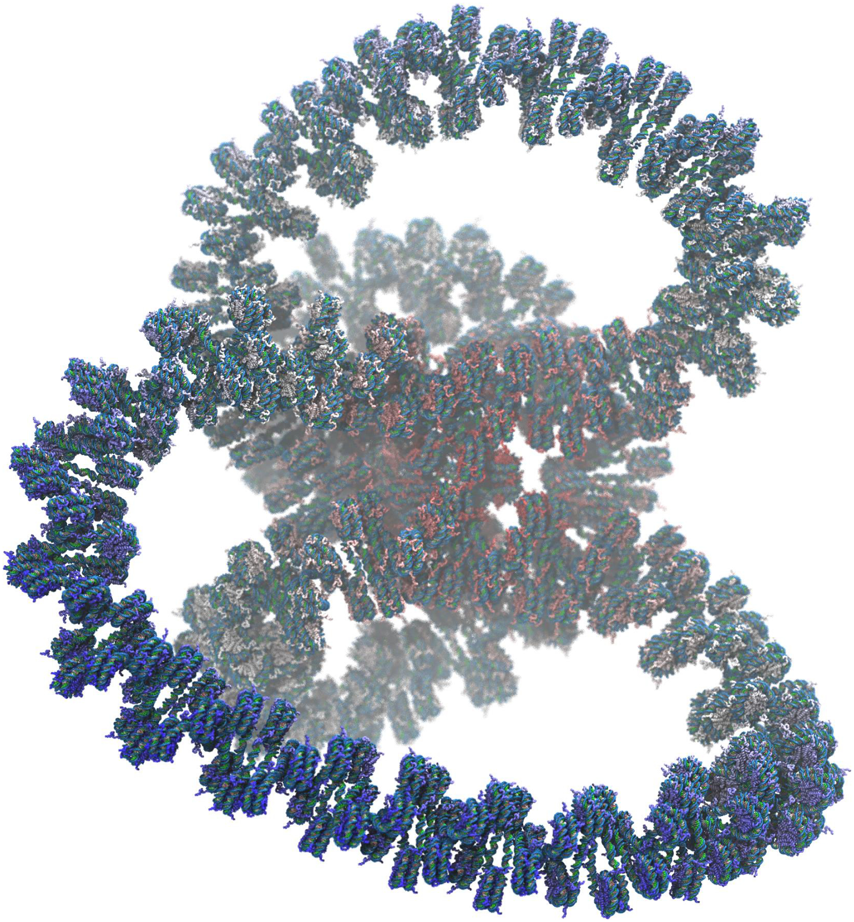
Structure of GATA4 gene, consisting of 83 kilobases of double stranded helical DNA wrapped around 427 nucleosomes. Protein tails used for programming gene expression protrude from each nucleosome.

II. METHODS

1. Atomistic model of GATA4 system

A. Modeling

We constructed a coarse-grained 3D scaffold using a coarse-grained mesoscale model of chromatin that led to the identification of a novel folding motif, hierarchical looping, where chromatin fibers undergo folding to produce layered networks of loops (citations to be added). By combining experimentally measured ultrastructural parameters with their previously verified mesoscale chromatin model, a detailed mesoscale model of the GATA4 gene locus was built (Figure 1) and used to derive atomic resolution coordinates. The model was equilibrated resulting in a compact globular structure exhibiting hierarchical looping, where the positions of the loops agree with 3C data, and local folding agrees in vivo experiments. Our mesoscale chromatin model consists of three particle types: linker DNA, nucleosome core particle pseudo-charges, and flexible histone tails.²³ Linker DNA is treated as a modified worm-like chain. The nucleosome core particles are represented as electrostatic objects, with shape and surface derived from the Discrete Surface Charge Optimization (DiSCO) algorithm that approximates the electric field of the atomic nucleosome by Debye-Hückel pseudo-charges along the surface of the complex as a function of monovalent salt.²⁴ Flexible histone tails are coarse grained so that 50 beads represent the 8 histone tails, where each bead represents about 5 amino acid residues.²³ The mesoscale model allows the direct placement of all-atom nucleosomal DNA and protein molecular structures in space, resulting in the atomistic model of the GATA4 system.

B. Automated clash detection for model generation of macromolecular complexes

Techniques such as X-ray crystallography, NMR spectroscopy and electron microscopy are just some of the methods used to determine protein structure. However, such experimental data is typically insufficient to build a fully atomistic model – one must combine experimental data with homology modeling techniques (a reconstruction of a protein structure based on its amino acid sequence and knowledge of the structure of a related homologous protein). The synthesis of homology techniques and experimental data is rarely flawless, and often steric clashes (which here we define as two atoms being separated by a distance less than 0.9Å) are introduced between atoms. This is highly undesirable as many molecular dynamics simulation packages are unable to correct for such clashes at the minimization stage and the high Van der Waals repulsion energy of the clashing atoms would lead to simulation failure. In light of this problem we develop a procedure to identify steric clashes in a general DNA-protein structure and automatically adjust atomic positions, without violating the known geometric constraints, such that all clashes are removed and corrected for. The DNA backbone is remarkably rigid. Besides the puckering behavior exhibited by the deoxyribose ring, the only other significant freedom of rotation lies in the phosphate group, about the O3’-C5’ axis. In principle this rotational freedom, denoted ɸ, can take on any value ɸ in [−180˚, 180˚), and this can be exploited for the purposes of clash correction (for geometric details see the work of Tung C.S. and Carter E.S.). Protein structures, unlike DNA, are generally more flexible, yielding more ways in which atomic positions can be modified to remove steric clashes. However, in practice we found that modifying just one torsion angle, denoted χ - where χ in [−180˚, 180˚), of the bond connecting the amino acid side-group to the residue was sufficient to remove all steric clashes in our models when combined with ɸ rotations. The clash correction program was predominantly written in Python, with calls to Fortran subroutines which calculate new atom positions upon changing ɸ or χ. Figure 2 shows a flow diagram of the program’s operation.

Figure 2.

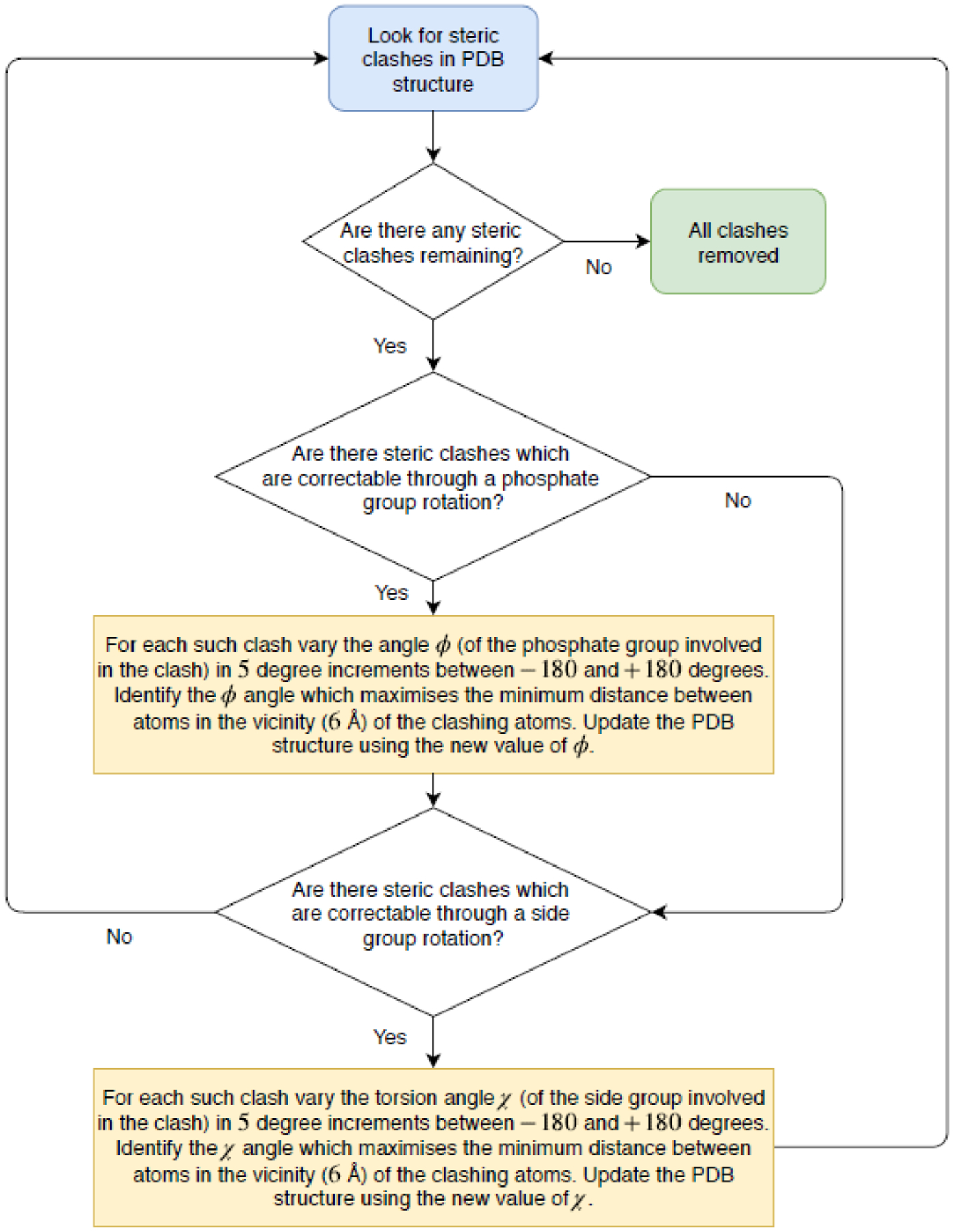
Automated clash detection: flow diagram of the operation of the clash correction script. Clashes correctable by a phosphate group rotation are those involving P, O5’, C5’, C4’, C3’, O3’ type atoms on the DNA backbone. All other clashes involve at least one atom in a protein side group, and can be corrected by a side group rotation. The vicinity of a clash is defined to be all atoms within a 6Å radius of the atoms involved in the clash.

2. Major characteristic of GENESIS for large-scale MD

For large-scale MD, GENESIS has the following major innovative characteristics:

A. Inverse lookup table²⁵

GENESIS makes use of a lookup table for energy and force evaluation of short-range non-bonded interactions instead of using direct calculations. The lookup table is based on the inverse distance squared calculation, which allows to perform accurate calculations for very short pairwise distances by assigning many table points, whereas fast evaluation of energy/force is available by reducing table points for longer pairwise distances.

B. Domain decomposition with midpoint cell method²¹

In the midpoint cell method, each rank has the data of cells in the corresponding subdomain and adjacent cells of the subdomains. It sends/receives data to/from the neighboring subdomains. The non-bonded interaction is parallelized by distributing the cell pair lists (or midpoint cell indices) over OpenMP threads. Integration and constraint evaluations are parallelized by distributing the cell indices in each subdomain over OpenMP threads. By adopting the midpoint cell method with the volumetric decomposition of FFT described below, we can assign the same domain decomposition between real- and reciprocal-spaces, skipping communications of charge grid data before FFT.

C. Volumetric decomposition of FFT²²

GENESIS makes use of the volumetric decomposition FFT where the reciprocal space is decomposed in all three dimensions. This requires more frequent MPI_Alltoall communications than slab or pencil decompositions. However, this scheme is more favorable for large systems on massively parallel supercomputers because the amount of data in each communication is much smaller than the other decompositions. Moreover, we can skip communication of charge data before FFT by assigning the same domain decompositions between real and reciprocal spaces. Specifically, let us assume that we decompose the overall space by P MPI processes. If P is factorized by P = P_x × P_y × P_z, we decompose the space by P_x in x dimension, P_y in y dimension, and P_z in z dimension. To perform the FFT in each dimension, we assign MPI_Alltoall communication such that each process has global data in the specified dimension. According to our volumetric decomposition FFT scheme (1d_Alltoall), forward FFT consists of eight computation/communication procedures outlined in Appendix.

In this scheme, we require five one-dimensional MPI_Alltoall communications. Intuitively, the procedure of the backward FFT (BFFT) is opposite to the forward FFT; this decomposition scheme has several advantages over other schemes from the scalability point of view despite of more frequent communications. On the one hand, the number of processes involved in communications is proportional to the cubic root of P. On the other hand, it is proportional to P or the square root of P in the case of slab or pencil decomposition FFT. When P is sufficiently large, the communication cost could be reduced by more frequent communication with small number of processes involved in the communication. We also utilize a volumetric decomposition scheme (see Appendix) with reduced frequency of communications while the number of processes involved in the communication is larger (2d_alltoall).

In this scheme, we require three one-dimensional MPI_Alltoall communications. The 2d_Alltoall scheme is similar to pencil decomposition FFT if we neglect the first MPI_Alltoallx communication. According to our investigations of 1d_alltoall and 2d_alltoall schemes, the performances are almost equivalent to each other on the K computer.

D. Parallel I/O for a large system¹⁹

For an MD simulation of a very large system, single restart/trajectory files cause several problems. First, there is a memory problem in reading single restart/trajectory files. In the case of a 1 billion atom system, we require a 24 GB (6 (three coordinates and velocities) × 1 billion (number of particles) × 4 (byte for a real number)) file size for a single restart file. Consequently, each process needs at least 24 GB memory to read only the restart file. Because we require not only restart but also PDB (protein data bank) and force-field parameter files, the file size becomes even larger than 100 GB, which can be prohibitively large. Writing a single restart/trajectory is even more problematic for a very large system. To write a single trajectory file, we need to accumulate 12 GB size coordinates by communication among processes. Parallel I/O is designed to avoid these problems. With parallel I/O, each process requires data of the corresponding subdomain. As we increase the number of processes, the required amount of data in each process decreases accordingly. A parallel restart file is generated from the initial PDB and parameter files using a parallel restart setup tool (prst_setup). During MD simulations, each MPI process writes trajectory files that contain only the coordinates of the corresponding subdomain. The number of files is identical to the number of MPI processes. After finishing the MD simulation, users can combine the trajectory files into a single file with atom selection option in order to only analyze the atoms/atom groups of interest.

3. Optimization of GENESIS for KNL Intel Xeon Phi processors

A. Hardware architecture of KNL in Trinity phase 2 and Oakforest-PACS

As the feature width of commodity chips approaches 10 nm, power consumption has increased substantially due to leakage currents. Many-core chips with fewer components per core and lower clock speeds therefore are being developed for future exascale computing. The 1.4 GHz Intel Knights Landing (KNL) 7250 chip in Trinity Phase 2 and Oakforest-PACS has 34 active tiles, each of which has two cores that share a single 1MB L2 cache. Each core supports four-fold simultaneous multithreading (SMT); thus, up to 272 hardware threads are available on a single node. They support AVX512 instructions including conflict detection, hardware gather/scatter prefetch, and exponential and reciprocal instructions. Each processor comes with 16 GB on-package High Bandwidth Memory (MCDRAM) and has access to an additional 96 GB memory via DDR4 channels. The MCDRAM and DDR support 400 GB/sec and 90 GB/sec streaming, respectively; however, the latencies of MCDRAM and DDR access are comparable. The memory mode of the processor is configurable at boot time; simulations were performed using nodes booted in the quad cache mode, in which the MCDRAM is configured as L3 cache, and the DDR is configured as usual. In Oakforest-PACS and Trinity Phase 2, Intel Omni-Path and Cray Aries interconnect are assigned, respectively.

B. Data Layout

In GENESIS 1.0–1.3 packages, coordinates, velocities and forces have an array-of-structures (AoS) type, in terms of source code organization. In other words, the x, y, and z components of coordinates, velocities, and forces are contiguous in memory. On KNL, the SIMD performance improves when making use of a structure-of-arrays (SoA) data type where x components of coordinates are contiguous in memory. To increase the SIMD performance, we changed the data layout from AoS to SoA in the module of real-space non-bonded interactions.

C. New Algorithm for real space non-bonded interactions: Reduced memory neighbor search scheme with improved performance

For the efficient usage of memory on KNL, we generate a new neighbor search scheme, which reduces the memory size significantly. In GENESIS 1.0–1.3 packages, we make use of the neighbor search algorithm based on the midpoint cell scheme. In this scheme, we first check cell pair indices icel and jcel for a given cell pair. For each atom indices i in icel, we search for atom indices j in jcel and write the indices of j as neighbor lists (Algorithm 1). The required memory size for the process becomes MN² for M cell pairs in a process and N atoms in a cell. The neighbor search is written every 10 or 20 steps, and the real space non-bonded interactions are performed based on this neighbor lists. For a very large system, this might make use of both MCDRAM and DDR, losing overall performance. Moreover, the algorithm does not allow contiguous memory access in force evaluation, preventing high SIMD performance (Figure 3(a)).

Algorithm 1.

Neighbor search used for GENESIS 1.0–1.3

do ij = 1, M M: number of cell pairs

icel = cell_index(1,ij) First cell index of the cell pair

jcel = cell_index(2,ij) Second cell index of the cell pair

do i = 1, N(icel) N(icel): Number of atoms in icel-th cell

do j = 1, N(jcel)

rij(1) = coord(1,i,icel)-coord(1,j,jcel)

rij(2) = coord(2,i,icel)-coord(2,j,jcel)

rij(3) = coord(3,i,icel)-coord(3,j,jcel)

dij = sqrt(rij(1)2+rij(1)2+rij(1)3)

if (dij < pairlist cutoff) then

Neighbor(i,ij) = Neighbor(i,ij) + 1

k = Neighbor(i,ij)

write Neighbor_list(k,i,ij)

end if

end do

end do

end do

Figure 3.

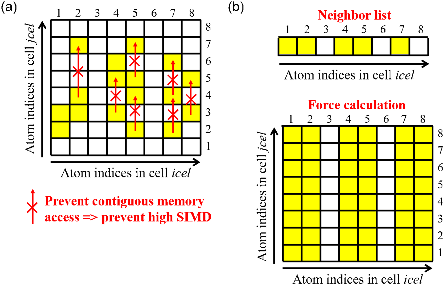
(a) Non-bonded interaction scheme used in GENESIS 1.0–1.3 and (b) new nonbonded interaction scheme for Intel Xeon Phi processors.

To use only MCDRAM in MD simulations with better performance, we devise a new algorithm of a neighbor search with reduced memory usage. In the proposed algorithm, for each atom i in icel, we check if there is at least one atom index j in jcel to be considered as a neighbor. If there is at least one neighbor of i, we write neighbor(i.ij)=1 in the neighbor search module. In the nonbonded interaction module, we assign interactions between i in icel with all j indices in jcel if neighbor(i,ij)=1. For example, let us consider atom index 5 in icel, shown in Figure 3. In this case, four atoms (indices 2, 4, 5, and 7) are considered as the neighbor list. In the new interaction scheme, we write neighbor(5,ij)=1 and calculate all interactions between 5-th atom in icel and all atoms in jcel in the non-bonded interaction module. In this neighbor search scheme, the required memory size becomes MN, so we can reduce the memory usage. This neighbor search scheme and the non-bonded interaction algorithm with SoA data is written in Algorithm 2. With our new neighbor search scheme, contiguous memory access is available, optimizing the overall performance (Figure 3(b)). Therefore, the new neighbor search scheme not only decreases the overall memory usage, but also results in better performance. In addition, this reduces the computational time of neighbor list writing because we are not required to check all particle pairs.

Algorithm 2.

Real-space non-bonded interaction kernel used for GENESIS 1.0–1.3

do ij = 1, M

icel = cell_index(1,ij)

jcel = cell_index(2,ij)

do i = 1, N(icel)

force_temp(1:3) = 0.0

do k = 1, Neighbor(i,ij) Number of neighbors of i-th atm in icel-th cell

j = Neighbor_list(k,i,ij) Neighbor of i-th atom in icel-th cell

rij(1) = coord(1,i,icel)-coord(1,j,jcel)

rij(2) = coord(2,i,icel)-coord(2,j,jcel)

rij(3) = coord(3,i,icel)-coord(3,j,jcel)

dij = sqrt(rij(1)2+rij(1)2+rij(1)3)

calculate f (1:3):force component from given distance

force_temp(1) = force_temp(1) – f (1)

force_temp(2) = force_temp(2) – f (2)

force_temp(3) = force_temp(3) – f (3)

force(1,j,jcel) = force(1,j,jcel) + f (1)

force(2,j,jcel) = force(2,j,jcel) + f (2)

force(3,j,jcel) = force(3,j,jcel) + f (3)

end do

force(1,i,icel) = force(1,i,icel) + force_temp(1)

force(2,i,icel) = force(2,i,icel) + force_temp(2)

force(3,i,icel) = force(3,i,icel) + force_temp(3)

end do

end do

D. Optimization of FFT with proper choice of the FFT decomposition scheme

In our previous development of the parallelization scheme, the FFT is performed on the K computer with 6D mesh/torus interconnect network. On the K computer, 1d_Alltoall and 2d_Alltoall schemes works almost equivalently by properly assigning the decomposition topology for the 1024³ PME grid. However, we could not guarantee the same parallel efficiency on the KNL machine. Therefore, one needs to investigate the parallel performance of the two developed schemes and make a choice of suitable FFT scheme for the target hardware and the target system.

III. Results and Discussion

1. Performance results of GENESIS on KNL

Although there are 68 cores per node, we assign 64 cores per node for easier selection of MPI processes. In each core, 4 threads are available. We considered 256 threads per node for our benchmark test. In our hybrid (MPI+OpenMP) parallelization, we assigned 8 OpenMP threads, so the number of MPI ranks in a node is fixed to 32. Benchmark systems are created by placing multiple STMV (Satellite tobacco mosaic virus) systems in a single box, and also by preparing the GATA4 gene locus system. We used the CHARMM force field with modified TIP3P explicit water model.^26,27 We used 12.0 Å cutoff thresholds, whereas van der Waals interactions were smoothed to zero from 10.0 Å to 12.0 Å using switch functions. We used the time step of 2 fs and neighbor list search and particle migrations were considered every 10 steps. Bonds related to hydrogen atoms were constrained by SHAKE/RATTLE algorithms.^28,29 The SETTLE constraint algorithm was used for the water.³⁰ On Oakforest-PACS, we investigated the parallel efficiency of our FFT scheme, and the effect of the new algorithms of the real-space non-bonded interactions from a 92,224 atom system (apolipoprotein A-I (ApoA1), a component of high-density lipoprotein). We also performed benchmarks using 1024³ and 2048³ PME grids for a 230 million and 1 billion atom model system. On Trinity Phase 2, we used a 2048³ grid for the GATA4 gene locus (1 billion atom system), but a smaller time step of 1 fs. In all cases, we used the Intel Fortran Compiler 17.0.

A. FFT communication time on Oakforest-PACS

To study the performance of GENESIS on KNL, we investigated the communication costs using the volumetric decomposition FFT schemes. Our target PME grid numbers here are 1024³ and 2048³. In MD simulations, these grid numbers are usually used for a system consisting of 100 million to one billion atoms. FFT timing statistics are obtained by running MD simulations: the communication time includes time of waiting before communication and all MPI_Alltoall communications. Because the PME grid number in the x dimension is not divisible by the number of processes (if the input grid number in the x dimension is n, the grid number in the x dimension becomes $\frac{n}{2}+1$ after the FFT by considering real-to-complex FFTs), each process has a different communication time. In Figure 4, we depict the timing statistics of total FFT execution and communications in FFT by choosing the time of the most time-consuming process. As mentioned in the previous section, we assigned 8 OpenMP threads, so the total number of threads used is obtained by multiplying 8 by the number of MPI processes. In the first step, the wait time could be large due to different starting setup times, so we measured the communicational time from 1001 to 2000 MD steps. This includes timing statistics of 1000 forward and backward FFTs. For both 1024³ and 2048³ PME grids, 2d_alltoall scheme is better than 1d_alltoall if the number of processes is not sufficiently large. On the other hand, 1d_alltoall becomes better than 2d_Alltoall for larger number of processes. Therefore, more frequent communications with small number of processes involved in the communication is preferred if we want to make use of large number of KNL processors. For the MD simulation of 1 billion atom size system with 2048³ PME grid sizes using more than 32768 MPI processes, 1d_Alltoall scheme is a better choice. This is different from the performance results of the K computer on which performances of 1d_Alltoall and 2d_alltoall are almost equivalent to each other even using very large number of MPI processes. The main difference between two tests on KNL and K is the number of MPI processor in a node: we used one MPI per node in the case of K whereas on KNL, 32 MPIs were assigned per node. We compared the FFT performance between our 1d_Alltoall and MKL FFT library used in GROMACS MD package version 2016.1, which makes use of the pencil decomposition FFT. Using MKL FFT, we observe that the lowest communication time of FFT for 2048³ grids is 34.22 ms, which is slightly higher than 1d_alltoall scheme (27.70 ms). From this comparison, we expect that 1d_alltoall could be the most suitable FFT parallelization scheme for a very large system on a large number of KNL processors.

Figure 4.

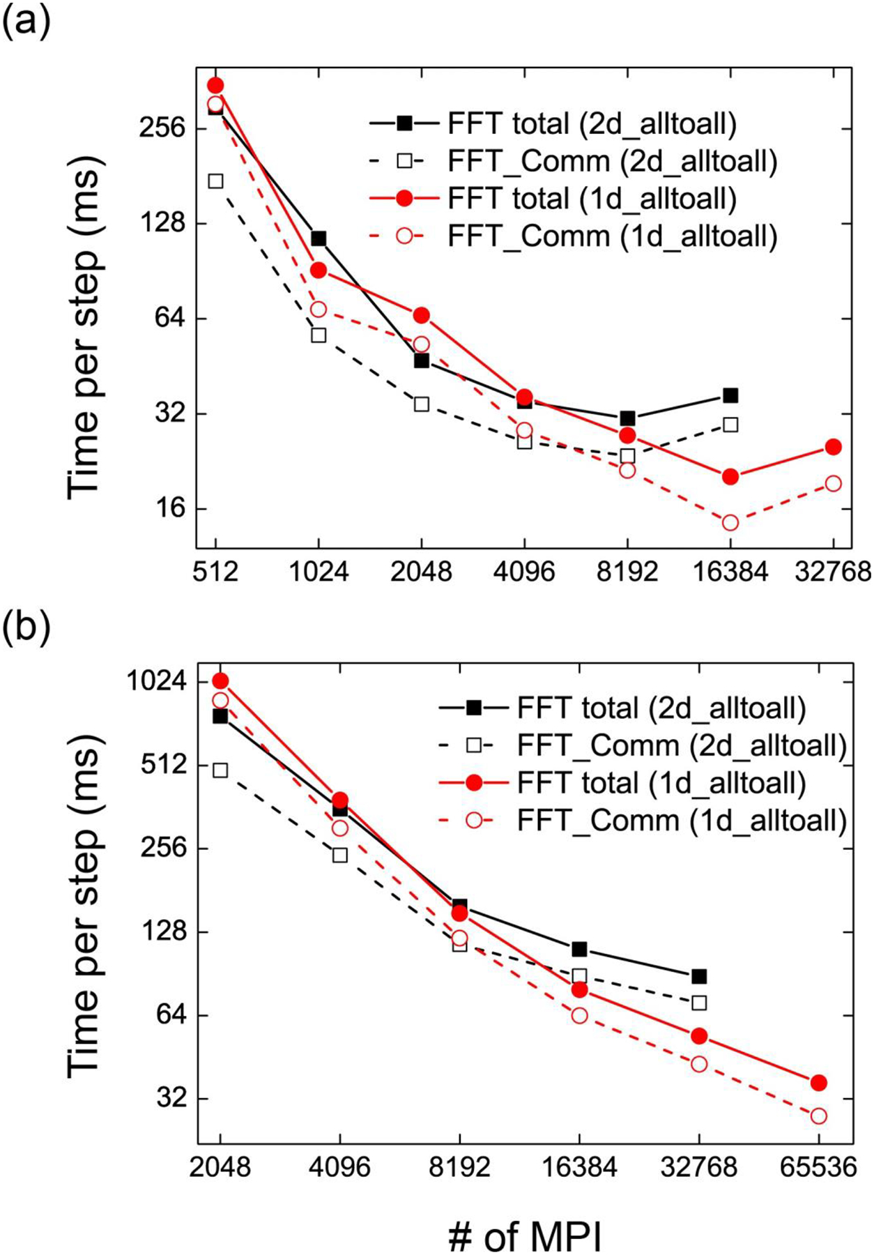
FFT time of (a) 10243 and (b) 20483 PME grids using GENESIS on Oakforest-PACS

B. Effect of new non-bonded interaction scheme with reduced memory

To understand the effect of the new neighbor search scheme with SoA data, we performed four MD simulations of ApoA1 (92,224 atoms) system on Oakforest-PACS: Algorithm 1 with and without AoS data and Algorithm 2 with and without SoA data. For one node, we assigned 32 MPIs with 8 OpenMP threads. The CPU time for the real-space non-bonded interactions and neighbor search generations are obtained from the profile of 0-th thread of the MPI rank 0 by using VTune Amplifier. In TABLE I, we show the memory usage for the neighbor search and the total number of pairwise interactions in real-space non-bonded interactions. In TABLE II, we describe the timing statistics of neighbor search generation and real-space non-boned interactions for 2000 MD steps. Here, we assigned the neighbor search list generation every ten steps. Our new algorithm (Algorithm 2 with SoA) has 1.5× better performance than that used in GENESIS 1.0–1.3 (Algorithm 1, AoS) although the number of interactions is 2.5 times larger and just one sixth of the memory is used for neighbor search. The higher speed of Algorithm 2 in the neighbor list is due to less computational cost. With Algorithm 1, we need to check all particle pairs. On the other hand, we can skip such a checking procedure frequently. The better performance of the real-space nonbonded interactions is mainly due to less L2 HW prefetcher allocations. With Algorithm 2 with SoA, the L2 HW prefetcher allocations are around 42000000. With Algorithm 1, this becomes 1.5 times larger. The large HW prefetch problem is highly related to the indirect memory access. With Algorithm 1, the index of the most inner loop is k, but we evaluate all interactions using index j by converting from the index k to j using neighbor_list. This indirect memory access becomes the main problem for performance improvement and can be reduced with Algorithm 2. We found that Algorithm 1 can be accelerated by adopting SoA data, but still shows less performance than Algorithm 2 because of the indirect memory access. Algorithm 2 with AoS data is 4x slower than the same algorithm with SoA, showing the importance of SoA data for performance. We also tested these algorithms on other CPU architecture: Intel’s Sandy bridge, Ivy bridge, Haswell, Broadwell, and Skylake micro-architectures, and SPARC64 VIIIfx on the K computer. For Haswell, Broadwell, and Skylake, Algorithm 2 works better than Algorithm 1. On the other hand, Algorithm 1 is better than Algorithm 2 for other processors. Even on Haswell, Broadwell, and Skylake, Algorithm 1 works better if we do not use INTEL compilers.

Table I.

Memory usage (GiB) for the neighbor search and number of pairwise interactions evaluated in real space nonbonded interactions (32 MPI with 8 OpenMP case)

	Memory usage	Number of interactions
Algorithm 1 (AoS)	305.88 MiB	47364470
Algorithm 1 (SoA)	305.88 MiB	47364470
Algorithm 1 (AoS)	48.40 MiB	122404436
Algorithm 1 (SoA)	48.40 MiB	122404436

Table II.

Calculation time (sec) of neighbor search + real-space nonbonded interaction for 2000 MD steps

	Neighbor List	Nonbond	Total
Algorithm 1 (AoS)	9.95	36.42	46.37
Algorithm 1 (SoA)	6.60	33.71	40.31
Algorithm 2 (AoS)	4.91	102.46	107.37
Algorithm 2 (SoA)	4.15	27.86	32.01

C. Benchmark of 230M and 1B system on Oakforest-PACS

Benchmarks of 230 million and 1 billion atoms (230M and 1B system) are performed by creating a system of 6×6×6 and 10×10×10 copies of STMV, respectively. As mentioned in Results Section 1 A-B, we applied 1024³ and 2048³ PME grids, corresponding to 1.2 Å and 1.0 Å PME grid spacings. We used velocity Verlet integrator with NVE ensemble, where the reciprocal-space calculation with FFT is performed every step. As shown in Figure 5, GENESIS shows good scalability even though we calculate reciprocal-space calculation every time step. The most time-consuming process is the evaluation of the real-space interaction for small numbers of processes. As we increase the number of MPI processes, the main bottleneck moves from the real-space to reciprocal space interactions because there is no communication in the real-space interaction while reciprocal-space interaction includes MPI_Alltoall communications in FFT. For example, in the case of 230M system using 2048 MPI ranks, the CPU time of real-space interaction is twice as large as the CPU time of reciprocal-space interaction. If we increase the number of MPI processes, the ratio of the CPU time becomes opposite: reciprocal-space interaction becomes twice of the real-space interaction. Due to our efficient FFT parallelization, we could reduce the CPU time of both real- and reciprocal-space non-bonded interactions, and obtain the scaling as shown in Figure 5.

Figure 5.

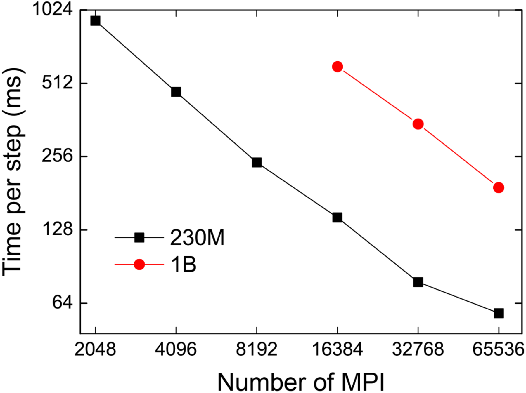
Benchmark performance of 230M and 1B system on Oakforest-PACS

D. MD simulation of the GATA4 system on Trinity Phase 2

On Trinity Phase 2, we performed 4 ns MD simulations of the gene locus with 1 fs time step. Parallel restart files are generated by “prst_setup” tool in GENESIS to reduce the file size required in each MPI rank. Here, we assigned 65536 MPIs, so the number of files is also 65536. The system size is 1907×2252×2485 ų, and it is subdivided by 32×32×64 subdomains according to the number of MPIs. Table III shows the timing statistics of each evaluation used in MD. Here, time for integration includes the time of integration of coordinates and velocities and that of communication of coordinates and forces. Bonded interactions consist of energy/force evaluation of bonds, angles, and dihedral angles. As shown in the table, the evaluation of non-bonded interactions takes around 80 % of the overall simulation time. For non-bonded interactions, the evaluation of the reciprocal-space interaction takes more than twice of the real-space interaction, and it covers more than 50 % of the simulation time. Communication times of forces and coordinates among subdomains are almost negligible. This observation suggests that the main problem of MD simulations of large systems on a large number of processors is the evaluation of the FFT included in the reciprocal-space interaction. We believe that our parallelization scheme of FFT is most suitable for large-scale MD simulations on a large number of processors, considering the scalability of our FFT.

Table III.

Calculation time (sec) of each component for 50 ps MD simulation of gene locus (time step is 1 fs)

	Total time (sec)	Ratio (%)
Total	9936.63	100.00
Integration	520.03	13.68
Bonded	13.68	0.14
Non-bonded (real)	2272.25	22.87
Non-bonded (reciprocal)	5493.88	55.29

2. Implications for chromatin biophysics: electrostatics of the crowded environment inside compacted chromatin

We performed the first billion atom biomolecular MD simulation of a gene locus in explicit solvent. The achievement is notable considering the necessity of including long-range forces, as well as the large memory footprint typically associated with biomolecular complexes, in contrast to large MD simulations in materials science, which typically neglect long-range forces. Importantly, the study is not only the first simulation of an entire gene locus, but also the first simulation of a gene to examine DNA sequence level. We note that electrostatics plays an important role in certain biological systems, including DNA, RNA, ion channels and chromatin complexes. Typically, electrostatic potentials are computed using the Poisson-Boltzmann method.³¹ While this method is excellent at characterizing the general features of the overall complex, many important aspects of electrostatic effects occur on short length scales, within the Debye length. Explicit solvent simulations allow us to more accurately simulate nucleosome-nucleosome interactions and nucleosome interactions with linker DNA, where charges are not fully screened by the ionic environment. In these regimes, the finite size and discrete nature of charged side chains, nucleic acid phosphates and ions themselves make important contributions, which are not described by the Poisson-Boltzmann approximation.³² In addition, the memory requirements of the Poisson-Boltzmann method are prohibitively expensive for very large systems such as the chromatin system studied in this work. Our simulations provide, for the first time, an example of short time scale dynamics of an entire gene consistent with a realistic force field potential and experimental data.

IV. Conclusions

Fully atomistic simulations based on coarse-grained models play a vital role for the understanding of chromatin structure. It is the properties of the structure on the atomic scale, such as how the DNA wraps around histone proteins to form nucleosomes and how the multiple nucleosomes wrap into a 30nm fiber that ultimately dictate the megabase-scale hierarchy of chromatin. It is also known that electrostatic interactions between dissolved ions and the fibers strongly affect folding dynamics, a process which can only be modelled on an atomistic level. Such studies enable the examination of histone tail dynamics, histone-histone and nucleosome-nucleosome interactions in crowded environments, all of which are important unsolved issues in chromatin dynamics and chromatin compaction, key processes in cell division, development, cancer and neuropsychiatric disorders. Improved calculations of the electrostatic potential will allow us to investigate the mechanism of interaction between histone tails of nearby nucleosomes, be it ion-mediated, water-mediated, direct charge-charge or some other as yet unknown mechanism.

Biomolecular simulations are particularly challenging computationally since they require the inclusion of long-range forces, which are often neglected in MD calculations in materials science. Here, we optimized the most time consuming real-space non-bonded interactions by using a simple neighbor scheme with reduced memory, contiguous memory access and change of data type from array of structures (AoS) to structure of arrays (SoA), particularly useful for the Intel Xeon Phi processor. We found that the new algorithm accelerates the speed by increasing SIMD performance. Long-range electrostatic interactions with the FFT were optimized by minimizing the number of processes involved in communications by volumetric decomposition. Our developments have been tested for 230 million atom and 1 billion atom systems with 1024³ and 2048³ PME grids, showing good parallel efficiency even when using more than 65,000 MPI proccesses, giving rise to the first billion atom simulation and also the first fully atomistic MD simulation of an entire gene.

Algorithm 3.

New neighbor search algorithm

do ij = 1, M

icel = cell_index(1,ij)

jcel = cell_index(2,ij)

Neighbor(i,ij) = 0

do i = 1, N(icel)

do j = 1, N(jcel)

rij(1) = coord(1,i,icel)-coord(1,j,jcel)

rij(2) = coord(2,i,icel)-coord(2,j,jcel)

rij(3) = coord(3,i,icel)-coord(3,j,jcel)

dij = sqrt(rij(1)2+rij(1)2+rij(1)3)

if (dij < pairlist cutoff) then

Neighbor(i,ij) = 1

exit the do loop

end if

end do

end do

end do

Algorithm 4.

Real-space non-bonded interaction kernel used for KNL

do ij = 1, M

icel = cell_index(1,ij)

jcel = cell_index(2,ij)

do i = 1, N(icel)

if (Neighbor(i,ij) == 0) cycle

force_temp(1:3) = 0.0 do j = 1, N (jcel)

rij(1) = coord(i,1,icel)-coord(j,1,jcel)

rij(2) = coord(i,2,icel)-coord(j,2,jcel)

rij(3) = coord(i,3,icel)-coord(j,3,jcel)

calculate f (1:3):force component from given distance

force_temp(1) = force_temp(1) – f (1)

force_temp(2) = force_temp(2) – f (2)

force_temp(3) = force_temp(3) – f (3)

force(j,1,jcel) = force(j,1,jcel) + f (1)

force(j,2,jcel) = force(j,2,jcel) + f (2)

force(j,3,jcel) = force(j,3,jcel) + f (3)

end do

force(i,1,icel) = force(i,1,icel) + force_temp(1)

force(i,2,icel) = force(i,2,icel) + force_temp(2)

force(i,3,icel) = force(i,3,icel) + force_temp(3) end do

end do

Appendix

Forward FFT with 1d_Alltoall scheme

MPI_Alltoall communication in x dimension (MPI_Alltoallx) FFT in x dimension (FFTx) MPI_Alltoall communication in x dimension (MPI_Alltoallx) MPI_Alltoall communication in y dimension (MPI_Alltoally) FFT in y dimension (FFTy) MPI_Alltoall communication in y dimension (MPI_Alltoally) MPI_Alltoall communication in z dimension (MPI_Alltoallz) FFT in z dimension (FFTz).

Forward FFT with 2d_Alltoall scheme

MPI_Alltoall communication in x dimension (MPI_Alltoallx) FFT in x dimension (FFTx) MPI_Alltoall communication in xy dimension (MPI_Alltoallxy) FFT in y dimension (FFTy) MPI_Alltoall communication in z dimension (MPI_Alltoallz) FFT in z dimension (FFTz).

References

- 1.McCammon JA; Gelin BR; Karplus M Nature 1977, 267(5612), 585–590. [DOI] [PubMed] [Google Scholar]
- 2.Narumi T; Ohno Y; Okimoto N; Koishi T; Suenaga A; Futatsugi N; Yanai R; Himeno R; Fujikawa S; Taiji M Proceedings of the 2006 ACM/IEEE conference on Supercomputing, 2006, pp 49. [Google Scholar]
- 3.Shaw DE; Deneroff MM; Dror RO; Kuskin JS; Larson RH; Salmon JK; Young C; Batson B; Bowers KJ; Chao JC; Eastwood MP; J. G; Grossman JP; Ho CR; J. ID; Kolossvary I; Kelpeis JL; Layman T; McLeavey MA; Moraes MA; Mueller R; Edward C; Shan Y; Spengler J; Theobald M; Towles B; Wang SC 34th Annual International Symposium on Computer Architecture (ISCA ‘07), 2007, pp 91–97. [Google Scholar]
- 4.Shaw DE; Grossman J; Bank JA; Batson B; Butts JA; Chao JC; Deneroff MM; Dror RO; Even A; Fenton CH Proceedings of the International Conference for High Performance Computing, Networking, Storage and Analysis, 2014, pp 41–53. [Google Scholar]
- 5.Shaw DE; Maragakis P; Lindorff-Larsen K; Piana S; Dror RO; Eastwood MP; Bank JA; Jumper JM; Salmon JK; Shan YB; Wriggers W Science 2010, 330(6002), 341–346. [DOI] [PubMed] [Google Scholar]
- 6.Harvey MJ; Giupponi G; De Fabritiis G J Chem Theory Comput 2009, 5(6), 1632–1639. [DOI] [PubMed] [Google Scholar]
- 7.Ruymgaart AP; Cardenas AE; Elber R J Chem Theory Comput 2011, 7(10), 3072–3082. [DOI] [PMC free article] [PubMed] [Google Scholar]
- 8.Pierce LC; Salomon-Ferrer R; Augusto F. d. O. C.; McCammon JA; Walker RC J Chem Theory Comput 2012, 8(9), 2997–3002. [DOI] [PMC free article] [PubMed] [Google Scholar]
- 9.Phillips JC; Sun Y; Jain N; Bohm EJ; Kalé LV Proceedings of the International Conference for High Performance Computing, Networking, Storage and Analysis, 2014, pp 81–91. [Google Scholar]
- 10.Abraham MJ; Murtola T; Schulz R; Pali S; Smith JC; Hess B; Lindahl E Software X 2015, 1–2, 19–25. [Google Scholar]
- 11.Brown WM; Carrillo JMY; Gavhane N; Thakkar FM; Plimpton SJ Comput Phys Commun 2015, 195, 95–101. [Google Scholar]
- 12.Jung J; Naurse A; Kobayashi C; Sugita Y J Chem Theory Comput 2016, 12(10), 4947–4958. [DOI] [PubMed] [Google Scholar]
- 13.Needham PJ; Bhuiyan A; Walker RC Comput Phys Commun 2016, 201, 95–105. [Google Scholar]
- 14.Eastman P; Swails J; Chodera JD; McGibbon RT; Zhao YT; Beauchamp KA; Wang LP; Simmonett AC; Harrigan MP; Stern CD; Wiewiora RP; Brooks BR; Pande VS PLoS Comput Biol 2017, 13(7). [DOI] [PMC free article] [PubMed] [Google Scholar]
- 15.Zhao GP; Perilla JR; Yufenyuy EL; Meng X; Chen B; Ning JY; Ahn J; Gronenborn AM; Schulten K; Aiken C; Zhang PJ Nature 2013, 497(7451), 643–646. [DOI] [PMC free article] [PubMed] [Google Scholar]
- 16.Yu I; Mori T; Ando T; Harada R; Jung J; Sugita Y; Feig M Elife 2016, 5, e19274. [DOI] [PMC free article] [PubMed] [Google Scholar]
- 17.Darden T; York D; Pedersen L J Chem Phys 1993, 98(12), 10089–10092. [Google Scholar]
- 18.Essmann U; Perera L; Berkowitz ML; Darden T; Lee H; Pedersen LG J Chem Phys 1995, 103(19), 8577–8593. [Google Scholar]
- 19.Jung J; Mori T; Kobayashi C; Matsunaga Y; Yoda T; Feig M; Sugita Y Wires Comput Mol Sci 2015, 5(4), 310–323. [DOI] [PMC free article] [PubMed] [Google Scholar]
- 20.Kobayashi C; Jung J; Matsunaga Y; Mori T; Ando T; Tamura K; Kamiya M; Sugita Y J Comput Chem 2017, 38(25), 2193–2206. [DOI] [PubMed] [Google Scholar]
- 21.Jung J; Mori T; Sugita Y J Comput Chem 2014, 35(14), 1064–1072. [DOI] [PubMed] [Google Scholar]
- 22.Jung J; Kobayashi C; Imamura T; Sugita Y Comput Phys Commun 2016, 200, 57–65. [Google Scholar]
- 23.Bascom GD; Sanbonmatsu KY; Schlick T J Phys Chem B 2016, 120(33), 8642–8653. [DOI] [PMC free article] [PubMed] [Google Scholar]
- 24.Zhang Q; Beard DA; Schlick T J Comput Chem 2003, 24(16), 2063–2074. [DOI] [PubMed] [Google Scholar]
- 25.Jung J; Mori T; Sugita Y J Comput Chem 2013, 34(28), 2412–2420. [DOI] [PubMed] [Google Scholar]
- 26.Huang J; MacKerell AD J Comput Chem 2013, 34(25), 2135–2145. [DOI] [PMC free article] [PubMed] [Google Scholar]
- 27.Price DJ; Brooks CL J Chem Phys 2004, 121(20), 10096–10103. [DOI] [PubMed] [Google Scholar]
- 28.Ryckaert JP; Ciccotti G; Berendsen HJ C. J Comput Phys 1977, 23(3), 327–341. [Google Scholar]
- 29.Andersen HC J Comput Phys 1983, 52(1), 24–34. [Google Scholar]
- 30.Miyamoto S; Kollman PA J Comput Chem 1992, 13(8), 952–962. [Google Scholar]
- 31.Baker NA; Sept D; Joseph S; Holst MJ; McCammon JA Proc Natl Acad Sci U S A 2001, 98(18), 10037–10041. [DOI] [PMC free article] [PubMed] [Google Scholar]
- 32.Hayes RL; Noel JK; Mohanty U; Whitford PC; Hennelly SP; Onuchic JN; Sanbonmatsu KY J Am Chem Soc 2012, 134(29), 12043–12053. [DOI] [PMC free article] [PubMed] [Google Scholar]