Automated mammographic breast density estimation using a fully convolutional network

Abstract

Purpose

The purpose of this study was to develop a fully automated algorithm for mammographic breast density estimation using deep learning.

Method

Our algorithm used a fully convolutional network, which is a deep learning framework for image segmentation, to segment both the breast and the dense fibroglandular areas on mammographic images. Using the segmented breast and dense areas, our algorithm computed the breast percent density (PD), which is the faction of dense area in a breast. Our dataset included full‐field digital screening mammograms of 604 women, which included 1208 mediolateral oblique (MLO) and 1208 craniocaudal (CC) views. We allocated 455, 58, and 91 of 604 women and their exams into training, testing, and validation datasets, respectively. We established ground truth for the breast and the dense fibroglandular areas via manual segmentation and segmentation using a simple thresholding based on BI‐RADS density assessments by radiologists, respectively. Using the mammograms and ground truth, we fine‐tuned a pretrained deep learning network to train the network to segment both the breast and the fibroglandular areas. Using the validation dataset, we evaluated the performance of the proposed algorithm against radiologists’ BI‐RADS density assessments. Specifically, we conducted a correlation analysis between a BI‐RADS density assessment of a given breast and its corresponding PD estimate by the proposed algorithm. In addition, we evaluated our algorithm in terms of its ability to classify the BI‐RADS density using PD estimates, and its ability to provide consistent PD estimates for the left and the right breast and the MLO and CC views of the same women. To show the effectiveness of our algorithm, we compared the performance of our algorithm against a state of the art algorithm, laboratory for individualized breast radiodensity assessment (LIBRA).

Result

The PD estimated by our algorithm correlated well with BI‐RADS density ratings by radiologists. Pearson's rho values of our algorithm for CC view, MLO view, and CC‐MLO‐averaged were 0.81, 0.79, and 0.85, respectively, while those of LIBRA were 0.58, 0.71, and 0.69, respectively. For CC view and CC‐MLO averaged cases, the difference in rho values between the proposed algorithm and LIBRA showed statistical significance (P < 0.006). In addition, our algorithm provided reliable PD estimates for the left and the right breast (Pearson's ρ > 0.87) and for the MLO and CC views (Pearson's ρ = 0.76). However, LIBRA showed a lower Pearson's rho value (0.66) for both the left and right breasts for the CC view. In addition, our algorithm showed an excellent ability to separate each sub BI‐RADS breast density class (statistically significant, p‐values = 0.0001 or less); only one comparison pair, density 1 and density 2 in the CC view, was not statistically significant (P = 0.54). However, LIBRA failed to separate breasts in density 1 and 2 for both the CC and MLO views (P > 0.64).

Conclusion

We have developed a new deep learning based algorithm for breast density segmentation and estimation. We showed that the proposed algorithm correlated well with BI‐RADS density assessments by radiologists and outperformed an existing state of the art algorithm.

1. Introduction

For over 30 years clinicians have used mammography for breast cancer screening. Research has shown that screening with mammography reduces breast cancer‐related deaths significantly, as noted with a 63% reduction among women who performed regular screening.¹ However, mammography is not perfect, as it suffers from lower sensitivity for women with dense breast tissue than for women with fatty breast tissue,² because of the potential masking of breast lesions by dense fibroglandular tissue. Women with dense breasts are often recommended to undergo additional screening procedures, such as magnetic resonance imaging (MRI) or ultrasound, which are more sensitive than screening mammography, but have lower specificity. In addition, research has shown that women with dense breasts are at higher risk for breast cancer than women with fatty breasts.^{3, 4} Assessing breast density from screening mammograms is an active area of research.

Among the various methods assessing breast density of women, the breast imaging reporting and data system (BI‐RADS)⁵ by the American college of radiology (ACR) is the most widely accepted classification method. Radiologists use the BI‐RADS density classification to assign women to one of four categories. The BI‐RADS (5th edition) breast density categories are: (a) entirely fatty, (b) scattered, (c) heterogeneously dense, and (d) extremely dense.

However, BI‐RADS breast density classification is subjective and coarse, and therefore, different radiologists can assign a different BI‐RADS density level to the same breast, especially for moderately dense breasts, which can be categorized as either scattered or heterogeneously dense. Thus, many previous studies (to name a few^{6, 7}) have established a relative proportion of dense fibroglandular tissue in a breast, referred to as breast percent density (PD), as an alternative to the four BI‐RADS categories.

To facilitate the process of estimating PD from a given FFDM, researchers have developed various automated algorithms. We can assign those algorithms into one of two categories: (a) area‐based or two‐dimensional methods^{6, 7, 8, 9} and (b) volumetric methods.^{10, 11, 12} Area‐based or two‐dimensional methods estimate PD from the proportion between the segmented breast area and the segmented dense fibroglandular areas in mammograms. Volumetric methods utilize the physics of x‐ray attenuations in breast tissue to estimate how much dense fibroglandular tissue exists in each given x‐ray path length. The area‐based PD is the most validated measure and researchers are actively using this measure, as indicated in recent studies.^{13, 14, 15} Among the above algorithms, Cumulus, a semi‐automatic area‐based method for estimating PD from the University of Toronto,⁶ is considered the gold standard for segmenting dense areas of the breast and estimating PD from given mammograms. However, Cumulus requires considerable human input and time to create the breast segmentation.

Laboratory for individualized breast radiodensity assessment (LIBRA), developed by Keller et al.⁷ at the University of Pennsylvania, is a fully automated algorithm for segmenting dense areas of the breast and estimating PD. LIBRA is a publicly available automated software that estimates area‐based PD by utilizing multiclass fuzzy C means to locate and segment dense fibroglandular areas. The software was validated against the area‐based PD from the mediolateral oblique (MLO) view of a mammogram estimated by radiologists using Cumulus. However, it may not always accurately segment the breast area, which can affect the PD estimate. Specifically, LIBRA uses a few connected straight lines to remove the pectoral muscle from the segmented breast area in the MLO view of a mammogram. However, the line between the pectoral muscle and the breast is not linear. Furthermore, LIBRA cannot remove nonbreast tissues, for example, belly tissue, imaged in the mammogram. These factors can hinder the accurate estimation of PD. These limitations are coming from the fact that humans set a list of rules for algorithms to follow. The algorithm fails if it encounters an event that is out of the predefined rules. This is a universal issue for automated algorithms built from human‐defined rules.

To overcome such limitations, researchers in computer vision and machine learning communities introduced deep learning, where the machine learns and determines the rules to solve given problems. Deep learning is a branch of machine learning, where multiple layers of artificial neural networks are trained using millions of (labeled) data to solve various data analysis problems, such as image classification and speech recognition, with the help of massive computing power via GPU. Since its first successful appearance in classifying natural scenes,¹⁶ deep learning has shown its effectiveness in various image analysis problems and it is now considered state of the art for various tasks in computer vision and machine learning fields. Researchers in the medical imaging field are now actively adopting deep learning to solve medical image analysis problems. Although there exists some areas of applications that deep learning outperforms medical professionals, for example, detecting diabetic retinopathy,¹⁷ deep learning in the medical imaging field is still in its infancy.

Previous studies for density segmentation using deep learning are very limited; Kallenberg et al. developed a convolutional sparse autoencoder (CSAE)¹⁸ to learn features in mammograms in an unsupervised fashion, and followed by a classifier on the learned features to solve a problem of interest, that is, mammographic density segmentation. They used manual segmentations of dense areas on mammograms by a radiologist as ground truth and evaluated the segmentation performance of their algorithm against the manual segmentations. They showed a good correlation (Pearson's rho of 0.85) between the PD computed from the manual segmentations and that from their algorithm's outputs. However, the dense area segmentation performance by their algorithm against that of the radiologist was suboptimal; the image wise averaged Dice coefficient¹⁹ was 0.63 with a wide confidence interval of 0.19.

In this study, we developed a new fully automated algorithm for mammographic breast density estimation using deep learning. Specifically, we used a deep learning framework developed for image segmentation, that is, fully convolutional network (FCN), which shows successful performance in segmenting objects in natural scenes,²⁰ to segment both the breast and the dense fibroglandular tissue areas from mammograms. We used manual segmentations of the breast area as ground truth. For dense area segmentation, we used a simple thresholding method based on BI‐RADS density assessments as ground truth. Then, we trained, tested, and validated our algorithm on FFDM exams of 604 women. As the size of our dataset is small compared to a typical dataset for deep learning, for example, ImageNet with over a million images with 1000 categories,²¹ we used a transfer‐learning method, that is, fine‐tuning, to train our algorithm. Then, we computed the PD using the segmented breast and dense area outcomes.

We compared the PD estimates of our algorithm against the BI‐RADS density assessments of radiologists to evaluate the segmentation performance of our algorithm. Specifically, we conducted a correlation analysis between the PD estimates of the proposed algorithm and radiologists’ BI‐RADS density assessments. In addition to the correlation analysis, we evaluated our algorithm's ability to classify BI‐RADS density levels using PD estimates, and the ability to provide consistent PD estimates for the left and the right breast, and for the MLO and CC views from the same women. To show effectiveness of our algorithm, we compared the performance of our algorithm to that of a state of the art and publicly available algorithm, LIBRA.

2. Methods

2.A. Dataset

Under an approved exempt institutional review board (IRB) protocol, we used screening mammograms of 604 women who underwent breast screening within the University of Pittsburgh Medical Center (UPMC) network during 2007 to 2013. The UPMC network uses the Hologic Selenia system (Hologic Inc, MA, USA) to obtain screening mammograms. All exams consisted of at least four views: left and right mediolateral oblique (MLO) views, and left and right craniocaudal (CC) views. We utilized those four views and the “for presentation” version of the mammograms for this study. Although the most current BI‐RADS version is the 5th edition, we acquired our data before this version was introduced, and therefore, radiologists reviewed the FFDM data of this study following the previous BI‐RADS edition (4th edition). Thus, we used the previous BI‐RADS edition for breast density assessments.

To develop and evaluate the proposed algorithm, among 604 women, we allocated the mammograms of mutually exclusive 455, 58, and 91 women into training, testing, and validation datasets (75%, 10%, and 15% of the entire exams), respectively. We grouped MLO and CC views together, but treated left and right mammograms as independent samples. Thus, the resulting mammogram images per view for each dataset were 910, 116, and 182, respectively. Table 1 summarizes the number of mammography images used for training, testing, and validating the proposed algorithm. We stratified the datasets in terms of BI‐RADS density level to show the breast density distribution of our dataset. We allocated similar number of cases for each density level for the validation set to increase the statistical power for classifying density level with low prevalence, that is, density level 1 and density level 4.

Table 1.

Characteristics of screening mammogram dataset

BI‐RADS density level (4th edition)	Training (N = 455)		Test (N = 58)		Validation (N = 91)
	MLO	CC	MLO	CC	MLO	CC
Density 1	60	60	8	8	30	30
Density 2	366	366	46	46	44	44
Density 3	454	454	58	58	56	56
Density 4	30	30	4	4	52	52
Total (# of mammogram images)	910	910	116	116	182	182

2.B. Establishing ground truth

To train a deep learning network to segment the breast and the dense fibroglandular areas, we first established ground truth for both the breast and the dense fibroglandular areas.

This study utilized manually segmented breast areas as the ground truth. Using a computer Graphic User Interface (GUI) tool in MATLAB (Mathworks, MA, USA), two undergraduate research assistants delineated the breast areas on mammograms in the dataset of this study (Fig. 1). We removed any nonbreast areas, such as the pectoral muscle and/or belly tissue, from the resulting ground truth mask for the breast area.

Figure 1.

Two undergrad research assistants delineated the breast area on mammograms using a GUI program in MATLAB. Created breast ground truth masks include only the breast area, removing the pectoral muscle, as shown in the right image, and/or belly tissue, as shown in the left image. [Color figure can be viewed at wileyonlinelibrary.com]

Then, within the manually segmented breast area, we established the ground truth for the dense fibroglandular area per image as follows:

1. Remove breast skin by applying a binary image erosion filter with a square structure with an edge length of 1 cm.

2. Create a histogram of the given breast area in terms of its gray‐level intensity.

3. Place a threshold in the histogram based on the BI‐RADS density of a given mammogram:

   1. Density 1: threshold at 87.5 percentile of the histogram

   2. Density 2: threshold at 62.5 percentile of the histogram

   3. Density 3: threshold at 37.5 percentile of the histogram

   4. Density 4: threshold at 12.5 percentile of the histogram

4. Assign any pixels with an intensity level higher than the given threshold as fibroglandular tissue.

We used the definition of the BI‐RADS density classification to create the above criteria. Note that radiologists reviewed the FFDM data of this study following the previous BI‐RADS edition (4th edition). According to the version of BI‐RADS density classification relevant to our data,²² the proportion of fibroglandular area in a mammogram increases every quartile (25%) as density level increases. Thus, the proportion of fibroglandular area in a histogram should increase as the BI‐RADS density level increases. That is, for breast with a BI‐RADS density level 1, we can expect that pixels in the last quartile in the intensity histogram would indicate dense fibroglandular area, while pixels in the last three quartiles would indicate dense fibroglandular area for a breast with BI‐RADS density level 3. Using this rationale, we assigned the midpoint of each quartile, that is, 12.5%, 37.5%, 62.5%, and 87.5% as the threshold value for each density category. Figure 2 shows examples how we setup the ground truth for dense breast tissue. Note that we used the midpoint of each quartile instead of the minimum or the maximum as the minimum or the maximum threshold will produce less meaningful dense area segmentation outputs for either density level 1 or 4 for training. For example, for density level 1, if we used 100% (i.e., maximum) as the threshold, it will segment nothing from the given breast area.

Figure 2.

This figure shows a few examples from each density level and mammographic view on how we established the ground truth mask for dense fibroglandular area. Images on the left side of the panel show the original mammograms. Images in the middle show the results after applying manually delineated breast area mask and skin removal using a binary image erosion technique. Then, we applied a thresholding method to get ground truth mask for dense fibroglandular area. We used the midpoint of quartiles, that is, 12.5, 37.5, 62.5, and 87.5 percentiles, of pixel intensity distribution as thresholds. Then, we assigned any pixels higher than a given threshold as dense fibroglandular area. Note that we selected thresholds in descending order based on each case's BI‐RADS density level. For example, we selected the 87.5 percentile as the threshold for BI‐RADS density level 1 cases. Images on the right side of the panel show the results after applying the thresholding method. Also shown are the pixel intensity histograms inside the breast area.

2.C. Fully convolutional network for breast and dense area segmentation

This study used an existing deep learning framework for segmentation, called fully convolutional network (FCN),²⁰ to segment the breast and the dense fibroglandular areas of the given breasts.

We used the VGG16 network²³ as our basic network structure and fine‐tuned the network for segmenting breast and dense areas using our dataset. As described in,²⁰ we removed the final classification layer of the VGG16 network and transformed the last two remaining fully connected layers to convolutional layers. Then, we added a 1 × 1 convolution layer with two channels to match our objective, which is assigning a pixel into either a foreground or background class. The resulting network provides a coarse score map for being a foreground or a background, since the original VGG16 network before the fully connected layer has five pooling layers with a stride of two, with a padding option for convolution to keep image resolution the same after convolution, which resulted in reducing the image size by a factor of 32. The resulting coarse score map then was upsampled with a transposed convolution layer with a stride of 32 to provide the segmentation score map for a given image. As the resulting output is too coarse to provide meaningful segmentation results, we utilized skip architecture to extract lower layer information to obtain high‐resolution segmentation outputs. We used the FCN‐8s,²⁰ which is a fused version of the output score map using the output of the final, pool4, and pool3 layers, as our final segmentation score map for a given image. To match the size of the output of the above three layers, we fused them in cascaded fashion; the final layer output is first upsampled with stride two and fused with the output of pool4, and then the resulting output upsampled with stride two again and fused with the output of pool3. At last, the resulting fused output is upsampled with stride 4. Note that each upsampling involves applying different transposed convolution layers. Following the original FCN paper,²⁰ we initialized the upsample layers to bilinear upsampling and then trained those weights during fine‐tuning. Table 2 shows the FCN network architecture used for this study.

Table 2.

VGG16‐based FCN network structure

Layer type	Kernel size	Stride	# Repetition	# Upsampling	Output
Output prediction FCN‐8s					A + B + C
Conv7	3 × 3	1 × 1		×4	A
Conv6	3 × 3	1 × 1
Max pool5	2 × 2	2 × 2		×2	B
Conv5	3 × 3	1 × 1	×3
Max pool4	2 × 2	2 × 2
Conv4	3 × 3	1 × 1
Max pool3	2 × 2	2 × 2		×1	C
Conv3	3 × 3	1 × 1	×3
Max pool2	2 × 2	2 × 2
Conv2	3 × 3	1 × 1	×2
Max pool1	2 × 2	2 × 2
Conv1	3 × 3	1 × 1	×2
Input image

2.D. Training (fine‐tuning) setup

The typical size of a mammogram is around 3000 × 4000 pixels. The purpose of this study is to segment the breast area and the dense area of the breast, which do not require the full resolution of a mammogram. Thus, we conducted the following preprocessing steps to train FCN networks:

• Convert an image I with 16 bit intensity [0, 65535] to an image $\widehat{I}$ with 8 bit intensity [0, 255] by using the following equation: $\widehat{I}=255\ast \tilde{I},\text{where}\tilde{I}=(I-\text{min}(I))/\text{max}(I).$

• Convert $\widehat{I}$ to RGB image $\overline{I}$ by repeating $\widehat{I}$ in red, blue, and green channels.

• Subsample images (original, breast area mask, and dense area mask) to 227 × 227 pixels.

The expected input image sizes for popular deep learning networks range from 224 × 224 to 299 × 299. For example, AlexNet¹⁶ expects to have a 227 × 227 input image size, while VGG16²³ expects 224 × 224, and Google's Inception model²⁴ expects a 299 × 299 input image resolution. Among these choices, we set 227 × 227 as an input image resolution, as it is enough to visualize the required information (e.g., dense area has higher pixel intensity than nondense area) for segmenting the breast and dense areas. However, it should be noted that one can choose other higher resolutions (e.g., 299 × 299 or higher) as input image size to train FCN networks.

We then trained four FCN networks, two (MLO and CC) for segmenting the breast area and two (MLO and CC) for segmenting the dense fibroglandular area. We refer to the two FCN networks for segmenting the breast area as FCN_BreastMLO and FCN_BreastCC, and the other two for segmenting the dense area as FCN_DenseMLO and FCN_DenseMLO. Note that we trained separate FCN networks for the MLO and CC views, as they contain anatomically different body parts. For example, the MLO view contains a pectoral muscle, which shows high intensity compared to other breast tissues, while the CC view typically contains only breast area. While it is possible to train a single network, we have chosen not to for this study. We trained all networks using the Adaptive Moment Estimation (Adam) optimizer²⁵ with a learning rate of 0.00001. We used a weight decay of 0.0005 for all layers and a dropout probability of 0.5 for the convolution layers 6 and 7. We set the batch size as 1 and augmented the training data by applying a random cropping by randomly moving a window up to 32 pixels in both the x and y axes. We followed the choice of the learning rate, weight decay, batch size, and dropout probability from a previous study,²⁶ which showed excellent results on a related, but different, task, that is, the segmentation of roads for Kitti Road Detection Benchmark.²⁷ We used cross‐entropy as a loss function and set the maximum iteration as 8000 for all networks. Every 100 iterations, we evaluated each FCN using the test dataset. Specifically, we tested each FCN by computing the Dice coefficient between the FCN outputs and corresponding ground truth. We found that both FCNs for breast area and FCNs for dense area converged and were steady when they were at the maximum iteration for the both training and testing datasets (Fig. 3). FCN_BreastMLO and FCN_BreastCC converged to a Dice score of 98–99 after 1000 iterations. FCN_DenseMLO and FCN_DenseMLO, are relatively slow to converge compared to FCN networks for breast areas, with the maximum Dice score of 94–95 after 4000 or 6000 iterations. Thus, we used the version of FCN networks at 4000 iterations for FCN_BreastMLO and FCN_BreastCC, while we used the version of FCN networks at 8000 iterations for FCN_DenseMLO and FCN_DenseMLO.

Figure 3.

This figure shows the testing scores, that is, Dice coefficient ranged [0, 100], for four FCN networks during the courses of training. Using the test dataset (N = 58 exams, that is, 116 MLO and CC view mammograms) we tested each network every 100 iterations of training. The plots include the Dice coefficient values for the training dataset (N = 455 exams, that is, 910 MLO and CC view mammograms). FCN networks for breast areas quickly converges to 98–99 after 1000 iterations for both the training and testing datasets. FCNs for dense areas relatively slow to converge compared to FCNs for breast areas, with the maximum Dice score for 94–95 after 4000 or 6000 iterations for both the training and testing datasets. We used the version of FCNs for breast areas at iteration 4000, and the version of FCNs for dense areas at iteration 8000 for this study.

2.E. Computing PD from segmentation outcomes

The output of the trained FCN networks is the probability map or score for each pixel being a foreground or a background. To convert the score map (ranged from 0 to 1) to a binary segmentation mask, we applied the threshold at 0.5. Note that one may see small blobs that are not the breast area in the output of FCN_BreastMLO and FCN_BreastCC. Thus, we selected the largest blob among all blobs in the output image as the breast area, and removed other smaller blobs from the output image. Figure 4 shows the flowchart of the proposed density segmentation algorithm of this study.

Figure 4.

This diagram summarizes the entire process of training, denoted as bold arrow lines, for the proposed algorithms, and how they create estimated breast area and dense area segmentations, denoted as dashed arrow lines. T refers to the thresholding to convert an estimated segmentation outcome in probability to binary masks. We used 0.5 for T. For breast area segmentation, we selected the largest blob in the resulting binary mask as breast area mask.

Using the segmented outcomes, that is, breast and dense area masks, we then computed the percentage density (PD) for each mammogram using the following equation:

$$PD=\frac{Area\left(DenseMask\right)}{Area\left(BreastMask\right)}.$$ (1)

2.F. Evaluation

We used the independent validation dataset, 182 MLO and CC view mammograms of 91 women, to evaluate the proposed algorithm.

We used BI‐RADS density assessments by radiologists as ground truth, and calculated the Pearson's correlation rho between it and the corresponding PD estimates by the algorithm. We computed the 95% confidence interval of the correlation coefficient using a bootstrapping over cases (N = 1000) in the validation set.

In addition, we evaluated whether the proposed algorithm has ability to separate given breasts into one of four BI‐RADS density categories. To do so, we first conducted one‐way analysis of variance (ANOVA) on both the proposed algorithm and LIBRA on PD estimates of all four BI‐RADS density categories, and then conducted a post hoc analysis using a multiple comparison test (multcompare function in MATLAB) using the one‐way ANOVA test statistics. In the multiple comparison test, we estimated the 95% confidence interval of the difference between the means of the two groups.

We also evaluated the algorithm's ability to provide consistent PD estimates for the same women, by comparing left and right, and MLO and CC views. We used Pearson's correlation analysis and Bland–Altman plot to evaluate the consistency of the algorithm.

In addition, we compared our algorithm against the state of the art and publicly available breast density segmentation algorithm, LIBRA, in terms of the above three evaluation criteria.

3. Results

Figure 5 shows four examples of breast and dense area segmentation outcomes from our proposed algorithm and LIBRA. Compared to LIBRA, the proposed algorithms delineated breast and dense areas better than LIBRA. For example, the proposed algorithm provided a smoother contour between the pectoral muscle and the breast than LIBRA, and it removed the skin effectively, while LIBRA assigned the skin area as the dense part of the breast.

Figure 5.

This figure shows some examples of breast area and dense area segmentation for the proposed algorithm and LIBRA. Images in 1st and 3rd columns show the outcomes of the proposed algorithm and those of LIBRA, respectively. Images in the center show the target mammograms. [Color figure can be viewed at wileyonlinelibrary.com]

Table 3 shows the summary statistics of the PD estimates from the proposed algorithm and LIBRA. The proposed algorithm computed similar PD estimates for the CC and MLO views (P‐value for mean difference was 0.2). However, LIBRA computed higher PD estimates for CC view cases, compared to those for the corresponding MLO view cases (P < 0.0001). In addition, we found that the PD estimates for the CC view from LIBRA was higher than those from the proposed algorithm (P < 0.0001). The above results indicate that the proposed algorithm estimated similar PD values for the CC and MLO views of the same breast, while LIBRA overestimated CC view cases over MLO view cases.

Table 3.

Summary statistics for PD estimates by the proposed algorithm and LIBRA

N = 91 exams (182 mammograms)	CC, Mean [95% CI] ± SD	MLO, Mean [95% CI] ± SD	CC − MLO Mean [95% CI]
Proposed	0.42 [0.4, 0.44] ± 0.14	0.41 [0.39, 0.44] ± 0.15	0.01 [−0.005, 0.03]
LIBRA	0.52 [0.49, 0.56] ± 0.21	0.44 [0.41, 0.47] ± 0.22	0.08 [0.06, 0.11]a
LIBRA – Proposed	0.1 [0.08, 0.13]a	0.03 [0.01, 0.06]

^aStatistically significant with significance level was 0.0125 after Bonferroni correction.

Then, we compared the PD values computed from each algorithm's output against radiologists’ BI‐RADS density assessments (Fig. 6). We observed high correlations²⁸ between the proposed algorithm's estimated PD values and the BI‐RADS density levels for CC and MLO views, respectively, while the correlations between LIBRA's estimates and the BI‐RADS density levels were only moderate for the same cases. In fact, LIBRA showed a low correlation coefficient for the CC view. Furthermore, the differences between the correlation values of the proposed algorithm and LIBRA for CC views were significantly different (Table 4).

Figure 6.

This figure shows the box plots of the proposed algorithm and LIBRA for the estimated PD values vs the BI‐RADS breast densities. The number of exams in each breast density category (density 1–4) are 15, 22, 28, and 26, respectively. The two extreme values on the box plots indicate the 25th and 75th percentile of the data. The two extreme values of the dash lines refer to the minimum and the maximum of the data that are not considered outliers. The plus (+) marker indicates a possible outlier within the data (which is more than 2.7 standard deviations above or below the mean of a normal distribution). The notches indicate the 95% confidence interval of the median.

Table 4.

Comparison of correlation values of the proposed algorithm and LIBRA. The correlation is between the PD estimates and radiologists’ BI‐RADS assessments

N = 91 exams (182 mammograms)	Proposed	LIBRA	Difference	P‐value
CC	0.81 [0.74, 0.85]	0.58 [0.43, 0.68]	0.24 [0.12, 0.41]	<0.0001a
MLO	0.79 [0.7, 0.85]	0.71 [0.57, 0.79]	0.08 [−0.02, 0.24]	0.18
CC‐MLO averaged	0.85 [0.8, 0.89]	0.69 [0.55, 0.77]	0.17 [0.08, 0.3]	0.006a

^aStatistically significant with significance level was 0.0167 after Bonferroni correction.

Both the proposed algorithm and LIBRA showed their ability to separate at least one BI‐RADS density class from other classes using their PD estimates (Table 5, all P‐values from one‐way ANOVA were approximately 0). However, the post hoc analysis results showed that the proposed algorithm had excellent ability to separate each sub‐BI‐RADS breast density class (Table 6); only one comparison pair, density 1 and density 2 in CC view, was not statistically significant. However, LIBRA failed to separate breasts in density 1 and 2 for both CC and MLO views. We found that LIBRA tended to overestimate the PD values for density level 1 and 2. In addition, we found that LIBRA was more susceptible for incorrect dense area segmentation than our algorithm for CC views with a BI‐RADS density level 1 [Fig. 6(b)]. We also observed the cases that LIBRA failed to segment dense area correctly for CC views with a BI‐RADS density level 1, resulting in a wide box plot for the corresponding density group.

Table 5.

One‐way ANOVA Statistics for PD estimates by the algorithms

View		Proposed algorithm					LIBRA
		SSa	df	MS	F	P‐value	SS	df	MS	F	P‐value
CC	Groups	2.41	3	0.8	141.38	7e‐47	2.99	3	0.996	32.97	5e‐17
	Error	1.01	178	0.006			5.38	178	0.03
	Total	3.42	181				8.37	181
MLO	Groups	2.63	3	0.88	104.7	4e‐39	4.78	3	1.59	72.47	1e‐30
	Error	1.49	178	0.008			3.91	178	0.22
	Total	4.12	181				8.69	181
Averaged	Groups	2.45	3	0.82	168.04	1e‐51	3.83	3	1.28	61.57	2e‐27
	Error	0.87	178	0.005			3.69	178	0.021
	Total	3.32	181				7.52	181

^aSS, df, and MS refer to sum of squares, degree of freedom, and mean square error.

Table 6.

Evaluation of the algorithm's ability to separate BI‐RADS density levels

View	BI‐RADS density level pairs	Proposed algorithm		LIBRA
		Mean difference and 95% CI	P‐value	Mean difference and 95% CI	P‐value
CC	1–2	−0.02 [−0.07, 0.02]	0.54	−0.05 [−0.15, 0.05]	0.64
	2–3	−0.12 [−0.16, −0.09]	<0.0001a	−0.11 [−0.2, −0.02]	0.0067
	3–4	−0.14 [−0.18, −0.11]	<0.0001a	−0.17 [−0.26, −0.09]	<0.0001a
MLO	1–2	−0.12 [−0.17, −0.06]	<0.0001a	−0.04 [−0.13, 0.05]	0.72
	2–3	−0.13 [−0.18, −0.09]	<0.0001a	−0.16 [−0.23, −0.08]	<0.0001a
	3–4	−0.08 [−0.13, −0.04]	<0.0001a	−0.22 [−0.29, −0.14]	<0.0001a
Averaged	1–2	−0.07 [−0.11, −0.03]	0.0001a	−0.04 [−0.13, 0.04]	0.59
	2–3	−0.13 [−0.17, −0.09]	<0.0001a	−0.14 [−0.21, −0.06]	<0.0001a
	3–4	−0.11 [−0.15, −0.08]	<0.0001a	−0.2 [−0.27, −0.12]	<0.0001a

^aStatistically significant with significance level of 0.0014 with Bonferroni correction. The mean difference for all other pairs, 1–3, 1–4, and 2–4 were statistically significant with P < 0.0001.

In addition, we averaged MLO and CC view PD estimates of both the proposed algorithm and LIBRA to obtain case‐based PDs (Fig. 7). The proposed algorithm showed high correlation with a Pearson's correlation ρ = 0.85 between the estimated PD values and the BI‐RADS density levels, while LIBRA only showed moderate correlation with a Pearson's correlation ρ = 0.69. The difference between the above two correlations were statistically significant (Table 4). We found that the proposed algorithm showed excellent ability to assess the BI‐RADS density level of the segmented dense area (Table 6). However, for LIBRA, the mean difference between BI‐RADS density 1 and 2 was not statistically different (Table 6).

Figure 7.

This figure shows the box plots of the proposed algorithm and LIBRA for the case‐based PD value, that is, MLO and CC view averaged, vs BI‐RADS breast density. The number of exams in each breast density category (density 1–4) is 15, 22, 28, and 26, respectively. The proposed algorithm showed higher correlation between the PD estimates and the BI‐RADS density levels than LIBRA.

Figures 8(a)–8(d) shows the Bland–Altman plot of the PD values for the left and right breasts estimated by the proposed algorithm and LIBRA. Both the proposed algorithm and LIBRA showed no systematical bias (mean difference < 0.02) between measures, except LIBRA for the PD estimates between the CC and MLO views (mean difference = −0.082), that is, LIBRA overestimated the PD estimates of the CC view compared to that of the PD view. However, LIBRA showed wider variations in the PD estimate differences than the proposed algorithm for all comparisons (i.e., for subplots A vs B, C vs D, and E vs F in Fig. 8). The correlation between the PD values of the left and right breasts for the proposed algorithm were high with a Pearson's correlation coefficient of 0.87 for the MLO view and 0.91 for the CC view. LIBRA showed a similar correlation level for the MLO view with a Pearson's correlation coefficient of 0.91. However, we found that LIBRA showed only a moderate level of correlation in the PD values between the left and right breasts for CC view, and the difference between the correlation coefficients of the proposed and LIBRA algorithms was statistically different (Table 7).

Figure 8.

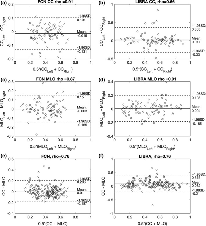
(a) and (c) show the Bland–Altman plot between the PD values of the left and right breasts for the proposed algorithm on MLO and CC views, respectively. Similarly, (b) and (d) show the Bland–Altman plots for LIBRA. (e) and (f) show the Bland–Altman plot between the PD estimates of CC and MLO views for the proposed algorithm and LIBRA, respectively. Note that the validation dataset (N = 91 exams, that is, 182 CC and MLO view mammograms) was used for this analysis. Both proposed and LIBRA showed no systematical bias (mean difference < 0.02) between measures, except LIBRA for the PD estimates between the CC and MLO views (mean difference = −0.082), that is, LIBRA overestimated PD estimates of the CC view compared to that of the MLO view. However, LIBRA showed wider variations in PD estimate differences than the proposed algorithm for all comparisons. The proposed algorithm showed high correlation (ρ > 0.87) between left and right PD value estimates for both MLO and CC views, while LIBRA showed only moderate correlation (ρ = 0.66) between left and right PD value estimates for CC views.

Table 7.

Comparison of the proposed algorithm and LIBRA for correlation in PD estimates between left and right, and MLO and CC view of same woman

Correlation (N = 91 exams, 182 mammograms)	Proposed	LIBRA	Difference	P‐value
PDLeft − PDRight, CC	0.91 [0.87, 0.94]	0.66 [0.4, 0.8]	0.25 [0.1, 0.49]	0.014a
PDLeft − PDRight, MLO	0.87 [0.78, 0.92]	0.91 [0.84, 0.94]	−0.04 [−0.12, 0.02]	0.73
PDCC − PDMLO	0.76 [0.66, 0.83]	0.75 [0.63, 0.83]	0.01 [−0.11, 0.13]	0.9

^aStatistically significant with significance level of 0.0167 with Bonferroni correction.

In addition, we found that both the proposed algorithm and LIBRA showed similar correlation level for their PD estimates from the CC and MLO views, with Pearson's correlation coefficient of 0.75–0.76. However, we found the difference in PD estimates between MLO and CC view from the proposed algorithm is smaller, with mean 0.07 ± 0.07, than those of LIBRA, with mean 0.12 ± 0.12. In fact, one can observe that PD estimates by our algorithm is closer to the mean than those of LIBRA [Figs. 8(e)–8(f)].

4. Discussion

We have shown that compared to LIBRA, our proposed algorithm can estimate PD consistently with radiologists’ BI‐RADS breast density categorization. It also has less variability and more consistency between views of the same breast and between views of the left and right breasts. In addition, LIBRA tended to have higher estimates of PD for dense breasts than those of the proposed algorithm (Figs. 6 and 7). The possible reason for the difference is the inclusion of skin for PD estimates. We specifically trained our algorithm to remove skin for dense area segmentation, while LIBRA did not enforce such a restriction. Previous research showed that including skin for PD in mammograms can increase the estimated PD by 3.8% to 4.9%.²⁹

Both our algorithm and LIBRA showed similar correlation in PD estimates between the MLO and CC views of the same breast. Although correlation coefficient values of 0.75–0.76 indicate strong correlation, the correlation amount is lower than that of a previous study, which ranged from 0.86 to 0.96.³⁰ For the case of our algorithm, some PD estimates for the CC view were higher than the corresponding MLO view, where the difference in PD estimates between them were higher than 0.25 [Fig. 8(e)]. These cases were part of the outliers. Specifically, two of these outliers were from BI‐RADS density level 1 cases and the remaining two were from BI‐RADS density level 4 cases. For those outliers with a BI‐RADS density 1 category, the proposed algorithm oversegmented the dense area in the CC view, while the proposed algorithm undersegmented the dense area in the MLO view for the outliers with a BI‐RADS density 4 category (Fig. 9). After removing the above four outliers, Pearson's correlation between PD estimates of the MLO and CC views were increased to 0.83, which is the upper bound of the 95% CI of Pearson's rho in Table 7.

Figure 9.

This figure shows outliers that the proposed algorithm either oversegmented (a)–(b) or undersegmented (c)–(d) dense fibroglandular areas of the breast. (a) and (b) are the right and left CC mammogram views from the same woman with a BI‐RADS density level 1. (c) and (d) are the right MLO mammogram views of two different women with a BI‐RADS density level 4. [Color figure can be viewed at wileyonlinelibrary.com]

Laboratory for individualized breast radiodensity assessment (LIBRA) showed poor performance on the CC view, while it showed compatible performance to the proposed algorithm on the MLO view. One possible reason is that LIBRA was optimized for the MLO view. In the original publication and its follow‐up research of LIBRA, the developers of LIBRA utilized the MLO view only^{7, 31} to segment dense area and estimate PD. Thus, one may need to avoid LIBRA to segment dense area and estimate PD from the CC view, as its performance on the CC view can be suboptimal.

We developed the proposed algorithm using a “for presentation” version of mammography exams from a single vendor (Hologic Inc), which may limit the proposed algorithm, as each vendor uses different image processing algorithms for presentation of mammography exams. Therefore, we, or others, should test the proposed algorithm on mammograms from other vendors to check the robustness of the proposed algorithm. It may be necessary to train the algorithm with cases from other vendors.

One may consider using BI‐RADS density ratings as ground truth as a potential limitation of this paper. This is because BI‐RADS density rating is an “indirect truth” for breast dense fibroglandular area segmentation. In fact, many previous studies^{7, 10, 11, 12} on breast density segmentation typically used manual segmentation of dense fibroglandular areas by radiologists as ground truth. However, it is well known that each radiologist is different from each other for segmenting dense breast area.³² In addition, most previous studies used segmentation outcomes from a very limited number of radiologists, typically one or two, as manual segmentation is time consuming and labor intense. Thus, it is possible that the density segmentation algorithms based on one or two radiologists are difficult to generalize for other radiologists and new cases. In this respect, the fact that we used indirect truth (i.e., BI‐RADS density rating by radiologists) to train our algorithm can be an advantage, not a limitation, over other previous algorithms using manual segmentations by one or two radiologists. We used BI‐RADS density ratings from a pool of radiologists, not just one or two radiologists, to create ground truth for dense fibroglandular area. As the PD estimates by our algorithm were highly correlated with BI‐RADS density ratings by a pool of radiologists, we concluded that our algorithm was able to locate and learn a common area or feature that a pool of radiologists would assess as the dense portion of the breast.

Another possible limitation of this study is that we used the fixed threshold value based on the BI‐RADS density ratings, for example, 12.5 percentile for BI‐RADS density 4, to obtain the ground truth segmentation for dense area. Thus, the resulting dense segmentation outcome can include error, either missing dense area or including nondense area, which can degrade the segmentation performance of the algorithm. However, we showed that deep learning could learn essential information to segment dense fibroglandular area, despite these possible errors on the ground truth for dense area. This is an important finding, especially for developing deep learning algorithms for image segmentation, as this may indicate that rough outlines for the region of interest may be enough to train deep learning algorithms for image segmentation. Thus, researchers may spend less time on establishing ground truth by trading off its precision. Of course, the required precision for image segmentation is different from one application to another. Future research is therefore required on the effect on the precision of ground truth for developing deep learning algorithms for image segmentation.

We used the VGG16 network as a basis deep learning architecture for this study. There are other deep learning architectures such as ResNet.³³ Although a previous study²⁶ reported that both VGG16 and ResNet showed similar performances on road segmentation benchmarks, there could be differences when applied to dense breast area segmentation. In addition, we can further optimize training parameters used for this study, such as learning rate and the threshold value to convert a score map to a binary segmentation (i.e., T in Fig. 4). We, or others, could conduct a follow‐up study of this paper by evaluating other network architectures and finding the optimal training parameters and threshold value.

In conclusion, we introduced a new deep learning‐based algorithm for breast density segmentation. We showed that the proposed algorithm can provide segmentation outcomes that its corresponding PD estimates are well correlated with radiologists’ BI‐RADS density assessments. In addition, we showed that the proposed algorithm outperformed the existing state of art algorithm, LIBRA.

References

- 1. Tabár L, Vitak B, Chen HH, Yen MF, Duffy SW, Smith RA. Beyond randomized controlled trials: organized mammographic screening substantially reduces breast carcinoma mortality. Cancer. 2001;91:1724–1731. [DOI] [PubMed] [Google Scholar]
- 2. Mandelson MT, Oestreicher N, Porter PL, et al. Breast density as a predictor of mammographic detection: comparison of interval‐ and screen‐detected cancers. J Natl Cancer Inst. 2000;92:1081–1087. [DOI] [PubMed] [Google Scholar]
- 3. Boyd NF, Guo H, Martin LJ, et al. Mammographic density and the risk and detection of breast cancer. N Engl J Med. 2007;356:227–236. [DOI] [PubMed] [Google Scholar]
- 4. Yaghjyan L, Colditz GA, Collins LC, et al. Mammographic breast density and subsequent risk of breast cancer in postmenopausal women according to tumor characteristics. J Natl Cancer Inst. 2011;103:1179–1189. [DOI] [PMC free article] [PubMed] [Google Scholar]
- 5. Sickles EA, D'Orsi CJ, Bassett LW. ACR BI‐RADS® mammography. In: D'Orsi CJ, eds. ACR BI‐RADS® Atlas: Breast Imaging Reporting and Data System. Reston, VA: American College of Radiology; 2013. [Google Scholar]
- 6. Byng JW, Boyd NF, Fishell E, Jong RA, Yaffe MJ. The quantitative analysis of mammographic densities. Phys Med Biol. 1994;39:1629–1638. [DOI] [PubMed] [Google Scholar]
- 7. Keller BM, Nathan DL, Wang Y, et al. Estimation of breast percent density in raw and processed full field digital mammography images via adaptive fuzzy c‐means clustering and support vector machine segmentation. Med Phys. 2012;39:4903–4917. [DOI] [PMC free article] [PubMed] [Google Scholar]
- 8. Glide‐Hurst CK, Duric N, Littrup P. A new method for quantitative analysis of mammographic density. Med Phys. 2007;34:4491–4498. [DOI] [PubMed] [Google Scholar]
- 9. Karssemeijer N. Automated classification of parenchymal patterns in mammograms. Phys Med Biol. 1998;43:365–378. [DOI] [PubMed] [Google Scholar]
- 10. Highnam R, Brady SM, Yaffe MJ, Karssemeijer N, Harvey J. Robust breast composition measurement – volparaTM. In: Martí J, Oliver A, Freixenet J, Martí R, eds. Digit Mammogr. Heidelberg: Springer; 2010:342–349. [Google Scholar]
- 11. Alonzo‐Proulx O, Packard N, Boone JM, et al. Validation of a method for measuring the volumetric breast density from digital mammograms. Phys Med Biol. 2010;55:3027–3044. [DOI] [PMC free article] [PubMed] [Google Scholar]
- 12. van Engeland S, Snoeren PR, Huisman H, Boetes C, Karssemeijer N. Volumetric breast density estimation from full‐field digital mammograms. IEEE Trans Med Imaging. 2006;25:273–282. [DOI] [PubMed] [Google Scholar]
- 13. Eng A, Gallant Z, Shepherd J, et al. Digital mammographic density and breast cancer risk: a case–control study of six alternative density assessment methods. Breast Cancer Res. 2014;16:439. [DOI] [PMC free article] [PubMed] [Google Scholar]
- 14. Burton A, Byrnes G, Stone J, et al. Mammographic density assessed on paired raw and processed digital images and on paired screen‐film and digital images across three mammography systems. Breast Cancer Res. BCR. 2016;18:130. [DOI] [PMC free article] [PubMed] [Google Scholar]
- 15. Jeffers AM, Sieh W, Lipson JA, et al. Breast cancer risk and mammographic density assessed with semiautomated and fully automated methods and BI‐RADS. Radiology. 2017;282:348–355. [DOI] [PMC free article] [PubMed] [Google Scholar]
- 16. Krizhevsky A, Sutskever I, Hinton GE. Imagenet classification with deep convolutional neural networks. In: Krizhevsky A, Sutskever I, Hinton GE, eds. Advances in Neural Information Processing Systems (NIPS). Red Hook, NY: Curran Associates, Inc.; 2012:1097–1105. [Google Scholar]
- 17. Gulshan V, Peng L, Coram M, et al. Development and validation of a deep learning algorithm for detection of diabetic retinopathy in retinal fundus photographs. JAMA. 2016;316:2402–2410. [DOI] [PubMed] [Google Scholar]
- 18. Kallenberg M, Petersen K, Nielsen M, et al. Unsupervised deep learning applied to breast density segmentation and mammographic risk scoring. IEEE Trans Med Imaging. 2016;35:1322–1331. [DOI] [PubMed] [Google Scholar]
- 19. Dice LR. Measures of the amount of ecologic association between species. Ecology. 1945;26:297–302. [Google Scholar]
- 20. Long J, Shelhamer E, Darrell T. Fully convolutional networks for semantic segmentation. In: Proc. IEEE Conf. Comput. Vis. Pattern Recognit. 2015: 3431–3440. [DOI] [PubMed]
- 21. Russakovsky O, Deng J, Su H, et al. ImageNet large scale visual recognition challenge. Int J Comput Vis. 2015;115:211–252. [Google Scholar]
- 22. American of College of Radiology and American of College of Radiology . Breast Imaging Reporting and Data System Atlas (BI‐RADS atlas). Reston, VA: American of College of Radiology, 98; 2003. [Google Scholar]
- 23. Simonyan K, Zisserman A. Very deep convolutional networks for large‐scale image recognition, ArXiv14091556 Cs; 2014.
- 24. Szegedy C, Vanhoucke V, Ioffe S, Shlens J, Wojna Z. Rethinking the inception architecture for computer vision, ArXiv151200567 Cs; 2015.
- 25. Kingma DP, Ba J. Adam: a method for stochastic optimization, ArXiv14126980 Cs; 2014.
- 26. Teichmann M, Weber M, Zoellner M, Cipolla R, Urtasun R. MultiNet: real‐time joint semantic reasoning for autonomous driving, ArXiv161207695 Cs; 2016.
- 27. Fritsch J, Kühnl T, Geiger A. A new performance measure and evaluation benchmark for road detection algorithms. In: Intelligent Transportation System‐(ITSC), 2013 16th Int. IEEE Conference on IEEE; 2013: 1693–1700.
- 28. Hinkle DE, Wiersma W, Jurs SG. Applied Statistics for the Behavioral Sciences, 5th edn. Boston: Houghton Mifflin, 2002. [Google Scholar]
- 29. Yaffe MJ, Boone JM, Packard N, et al. The myth of the 50‐50 breast. Med Phys. 2009;36:5437–5443. [DOI] [PMC free article] [PubMed] [Google Scholar]
- 30. Byng JW, Boyd NF, Little L, et al. Symmetry of projection in the quantitative analysis of mammographic images. Eur J Cancer Prev. 1996;5:319–327. [DOI] [PubMed] [Google Scholar]
- 31. Keller BM, Chen J, Daye D, Conant EF, Kontos D. Preliminary evaluation of the publicly available Laboratory for Breast Radiodensity Assessment (LIBRA) software tool: comparison of fully automated area and volumetric density measures in a case‐control study with digital mammography. Breast Cancer Res. 2015;17:117. [DOI] [PMC free article] [PubMed] [Google Scholar]
- 32. Keller BM, Nathan DL, Gavenonis SC, Chen J, Conant EF, Kontos D. Reader variability in breast density estimation from full‐field digital mammograms. Acad Radiol. 2013;20:560–568. [DOI] [PMC free article] [PubMed] [Google Scholar]
- 33. He K, Zhang X, Ren S, Sun J. Deep residual learning for image recognition. In 29th IEEE Conference on Computer Vision and Pattern Recognition CVPR. Las Vegas; 2016.