Imaging brain function with simultaneous BOLD and viscoelasticity contrast: fMRI/fMRE

Abstract

Magnetic resonance elastography (MRE) is emerging as a new tool for studying viscoelastic changes in the brain resulting from functional processes. Here, we demonstrate a novel time series method to generate robust functional magnetic resonance elastography (fMRE) activation maps in response to a visual task with a flashing checkerboard stimulus. Using a single-shot spin-echo (SS-SE) pulse sequence, the underlying raw images inherently contain blood-oxygen-level dependent (BOLD) contrast, allowing simultaneous generation of functional magnetic resonance imaging (fMRI) activation maps from the magnitude and functional magnetic resonance elastography (fMRE) maps from the phase. This allows an accurate comparison of the spatially localized stiffness (fMRE) and BOLD (fMRI) changes within a single scan, eliminating confounds inherent in separately acquired scans. Results indicate that tissue stiffness within the visual cortex increases 6–11% with visual stimuli, whereas the BOLD signal change was 1–2%. Furthermore, the fMRE and fMRI activation maps have strong spatial overlap within the visual cortex, providing convincing evidence that fMRE is possible in the brain. However, the fMRE temporal SNR (tSNR_fMRE) maps are heterogeneous across the brain. Using a dictionary matching approach to characterize the time series, the viscoelastic changes are consistent with a viscoelastic response function (VRF) time constant of 12.1 s ± 3.0 s for a first-order exponential decay, or a shape parameter of 8.1 s ± 1.4 s for a gamma-variate.

1 |. INTRODUCTION

Modern functional neuroimaging techniques have greatly advanced the field of neuroscience, with different modalities targeting distinctive aspects of brain physiology, functional architecture, and dynamics. Specifically, functional magnetic resonance imaging (fMRI) uses blood-oxygen-level dependent (BOLD) contrast [1] to study the underlying neurovascular coupling, which links neuronal activity to an increase in local blood oxygenation. In this study, we introduce a novel method for functional magnetic resonance elastography (fMRE) to observe a different coupling mechanism—neuromechanical coupling, where neuronal activity is linked to an increase in local brain tissue stiffness. The novelty in our approach comes from utilizing a time series acquisition, similar in concept to that employed in fMRI, where the magnitude and phase information from the time series can be submitted to separate processing and analysis to arrive at fMRI and fMRE activation maps, or statistical parametric maps (SPMs). Since our simultaneous fMRI-fMRE method is both multi-modal and concurrent, it allows us to compare the spatially localized BOLD and stiffness changes within the same scan, eliminating confounds inherent in separately acquired scans.

1.1 |. Magnetic Resonance Elastography

Brain tissues are viscoelastic (VE), and their shear modulus (“stiffness”) properties can be measured via magnetic resonance elastography (MRE), a noninvasive imaging technique that uses phase-contrast MRI to quantitatively assess tissue mechanical properties [2, 3]. The technique involves three steps: (1) generating shear waves in the tissue of interest; (2) imaging the wave propagation with MRI; (3) processing the shear wave images to generate quantitative stiffness maps, also referred to as elastograms. A gradient-echo (GRE) or spin-echo (SE) MRI sequence is used with added motion-encoding gradients (MEGs) that are switched in polarity and phase to match the tissue vibration frequency. This causes any cyclic motion in the direction of the MEGs to yield a measurable phase shift in the MR signal. The phase shift can be used to derive the tissue displacement at each voxel to generate images of the shear wave propagation. These wave images are then processed with a reconstruction algorithm (either direct or iterative) that solves the inverse problem of the wave equation to compute the complex shear modulus, G* = G′ + iG″, where G′ is the shear storage modulus and G″ is the shear loss modulus [4, 5]. The calculated complex shear modulus map is a quantification of the tissue viscoelastic properties. In our study, the absolute value of the complex shear modulus is utilized, which corresponds to the “stiffness” parameter perceived in palpation exams. These viscoelastic parameters are used by physicians and researchers to assess tissue properties and to diagnose diseases in organs including the liver [6, 7, 8], kidney [9, 10], breast [11, 12, 13], skeletal muscle [14], and brain [15, 16].

Developments in the brain MRE techniques have mainly focused on deriving the shear stiffness of global brain tissue and specific neuroanatomical regions (e.g., deep gray matter [17]). An increasing number of studies have been conducted to understand how brain stiffness changes as a function of healthy aging [18, 19], gender differences [18, 19], and neurodegeneration (e.g., multiple sclerosis and Alzheimer’s disease [20, 21, 22]). In general, the brain softens with age and neurodegeneration, with specific changes depending on the region, and occipital and temporal lobes are stiffer in females than in males.

1.2 |. Previous Functional MRE

Recently, MRE has been applied to functional studies in the brain to explore whether there are mechanical changes in localized regions modulated by cognitive processes in an attempt to uncover a new functional contrast mechanism in the brain. The first human fMRE study used a serial sequence design to look at the correlation between the stiffness and visual stimulus at different mechanical driving frequencies in 57 volunteers. They found a diffuse decrease in viscoelastic response due to visual stimulation that is not localized to the visual cortex [23]. In the 2015 single-subject studies, the stimuli were presented on minute-long time scales, with the human motor cortex decreasing in stiffness with finger tapping [24] and the mouse sensory cortex increasing in stiffness with a 1-kHz auditory stimulus [25]. As the authors described, the difference in the sign of the stiffness changes could be due to differences in habituation, imaging vibration frequencies, cortical regions imaged, and influence of anesthesia. In 2017, these investigators introduced an interleaved paradigm of 10-s experimental stimulus ON/OFF and a control OFF/OFF scan so that 4 elasticity maps, one for each condition, were obtained for each subject [26]. They reported a regional stiffness increase of 14% when averaged across 7 mice with hind-limb electric stimulation. In the most recent studies [27, 28, 29], different interleaving stimulus frequencies were used in mice and human brains. The results still indicated a 10–20% increase in shear modulus, and they observed an additional increase in stiffness when the visual stimulus was switched off. In these studies, the statistical estimation of fMRE changes was performed by averaging across the subjects, since each ON or OFF condition only resulted in a single elastogram. In our study, we used block trials, similar to [23], and time series analysis in a single scan to enhance the statistics on a single-subject basis.

1.3 |. Time Series

The time series method has been used in fMRI since its inception as a way to detect the small signal changes characteristic of BOLD contrast. Treating fMRI data in a time series manner allows for the use of general linear model (GLM) analysis, an efficient method to perform statistical analysis, the aim of which is to determine which voxels have a time course that correlates with the applied pattern of stimulation or experimental manipulation.

In order to acquire a functional time series in a reasonable amount of time, a fast single-shot imaging sequence with a short repetition time (TR) is used, such as a spiral or echo-planar imaging (EPI) acquisition. In addition to the resulting GLM statistics that estimate the viscoelastic tissue activation changes, other parameters can be derived as quality indicators from the time series, including temporal signal-to-noise ratio (tSNR), contrast-to-noise ratio (CNR), percent signal change, average signal, standard deviation, and autocorrelation of the static spatial noise. In addition, we introduce a dictionary matching approach [30] to characterize a heuristic model of fMRE dynamics.

1.3.1 |. General Linear Model

In the general linear model (GLM) approach, the signal time-course of each voxel is modeled as a weighted sum of one or more known predictor variables, also referred to as regressors, plus an error term. The GLM can be written in the following matrix form:

$$y=X\beta +\epsilon$$

where y is the time series signal associated with a single voxel, X is the design matrix in which each column is a predictor variable, β is the parameter vector or regressor, and ϵ is the error vector in which each value is the error associated with each observation/measurement [31]. For a simple task fMRI analysis, the regressor usually consists of the block design convolved with a hemodynamic response function (HRF), e.g. [32]. The HRF represents the BOLD response to a short (impulsive) stimulus. In this work, we introduce the analogous quantity in fMRE, the viscoelastic response function (VRF) to characterize the stiffness changes resulting from a short cognitive stimulus.

The goal of the analysis is to describe the variability in the time series data in terms of experimental parameters, confounding effects, and residual noise. Statistical tests are then performed on a voxel-by-voxel basis, where the model parameters β are compared to the standard error. When β is large compared to the standard error, defined as when the t-score is above a certain preset significance threshold, the null hypothesis is rejected, and the voxel is “activated.” The collection of these univariate analyses over all voxels of the volume then paints what is commonly called an activation map.

2 |. MATERIALS & METHODS

2.1 |. Subjects

Eleven healthy right-handed volunteers (8 males and 3 females, age range: 22–35 years old) recruited from the Stanford community were scanned on a 3T scanner (Discovery MR 750, GE Healthcare, Waukesha, WI, USA) after granting written informed consent under a protocol approved by the Stanford Institutional Review Board.

2.2 |. Visual Task

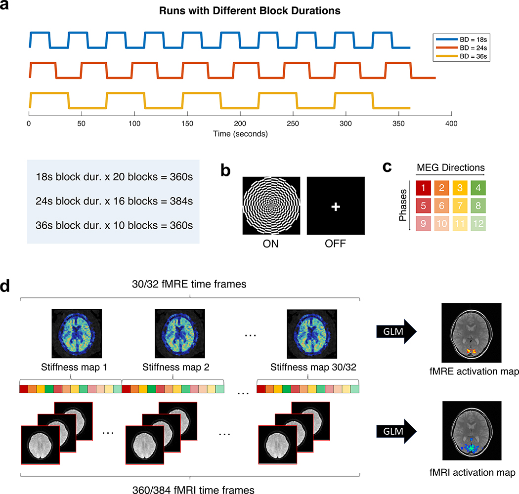
The functional scans were acquired using a block-design paradigm, alternating between a visual task (ON block) and rest (OFF block). Each subject underwent 3 runs of functional task scans with block durations of 18 seconds (20 blocks), 24 seconds (16 blocks), and 36 seconds (10 blocks), in randomized order (Fig. 1a). The ON or task block consists of a contrast-reversing checkerboard visual stimulus flickering at 10 Hz; the OFF or rest block is a fixation cross (Fig. 1b). Stimuli were presented using E-Prime software (Psychology Software Tools, Pittsburgh, PA, USA).

FIGURE 1.

(a) Each subject underwent 3 runs of the visual task with different block durations (BD). (b) The ON block is a contrast-reversing checkerboard flickering at 10 Hz, and the OFF block is a fixation cross. (c) The MRE sequence consists of 4 motion-encoding gradient (MEG) directions (red, orange, yellow, green) and 3 phase offsets (varying tints) to generate one stiffness map. (d) Depending on the block duration, 30/32 stiffness time frames and 360/384 fMRI time frames were simultaneously acquired for a total acquisition time of 360/384 s. GLM analysis was performed to generate fMRE and fMRI activation maps.

2.3 |. Data Acquisition

Shear waves at 60 Hz were induced in the brain using a pneumatic actuator connected to a soft, pillow-like passive driver placed under the subject’s head (Resoundant, Mayo Clinic, Rochester, MN, USA) inside a standard 8-channel receive-only coil as described by Murphy et al. [22]. The resulting tissue motion was imaged with a single-shot, spin-echo echo-planar imaging (SS-SE-EPI) sequence with the following parameters: 12 oblique-axial slices, TR/TE = 1000/64.5 ms, FOV = 22 cm, BW = ±250 kHz, 72 × 72 imaging matrix reconstructed to 128 × 128, 2x ASSET acceleration, 3.5 mm thick slices with zero slice gap, one 0th- and 1st-order moment nulled motion-encoding gradient lobe on each side of the refocusing radiofrequency (RF) pulse synchronized to the motion, Hadamard motion-encoding (4 directions of motion-encoding gradients (MEGs)) [33], and 3 phase-offsets sampled over one period of motion at 60 Hz (16.67 ms). The sequence of 4 MEGs × 3 phases resulted in a 12 s fMRE repetition time (TR_fMRE) to acquire a single time frame of fMRE data (Fig 1c and 1d), which was repeated 30 or 32 times for a total acquisition time of 360 s or 384 s, respectively, depending on the block duration (30 time frames for 18 s and 36 s block duration; 32 time frames for 24 s block duration) (Fig 1a). The slice prescription spanned each subject’s primary visual cortex (V1), where the bottom-most slice begins at the calcarine sulcus.

T₂-weighted fast spin echo structural images were acquired for anatomical reference using the same slice prescription as the functional scans and the following parameters: TR/TE = 3000/68 ms, ETL = 12, 192 × 256 matrix size.

2.4 |. Data Processing and Analysis

Image processing and analysis were performed using FMRIB Software Library (FSL, V5.0.10) [34] FMRI Expert Analysis Tool (FEAT) procedures [35] and MATLAB (Mathworks, Natick, MA, USA).

2.4.1 |. fMRI

Preprocessing

The fMRI time series was generated by taking the magnitude of the T₂-weighted raw spin-echo images (TR_fMRI = 1 s; total of 360 or 384 time frames). The following preprocessing was conducted using FSL FEAT: motion correction via MCFLIRT [36], slice timing correction, brain extraction via BET [37], and 0.01 Hz high-pass filtering. No spatial or temporal smoothing was performed.

Analysis

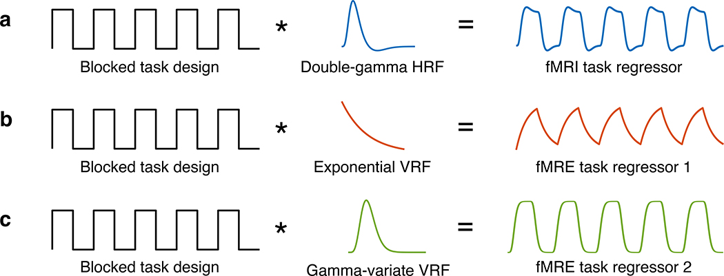
The preprocessed T₂-weighted fMRI time series was submitted to FILM GLM analysis. FILM prewhitening was conducted to account for temporal autocorrelation. The task regressor was a boxcar function, corresponding to the block design stimulus, convolved with a double-gamma HRF [32] (Fig. 2a).

FIGURE 2.

Schematic for the generation of fMRI and fMRE task regressors. (a) The fMRI task regressor is a boxcar function (corresponding to the task ON and OFF blocks) convolved with a canonical hemodynamic response function (HRF). (b & c) The fMRE task regressors for a first-order exponential decay model and gamma-variate model is a boxcar function convolved with an exponential viscoelastic response function (VRF) and a gamma-variate VRF, respectively.

2.4.2 |. fMRE

Stiffness Reconstruction

Complex-valued images containing the motion in the X, Y, and Z directions were calculated from the 4 MEG directions for each phase. These volumes were smoothed in the Z direction using a 1D, 4th-order, Butterworth, low-pass filter with a cut-off frequency of 3 cycles per FOVz to reduce potential slice-to-slice phase jitter. The curl of the smoothed vector wave field was calculated using 3×3×3-element, central-difference, derivative kernels for each MRE time point. Each MRE data set then contained curl wave images at each of 3 MRE phase offsets evenly spaced over 1 period of the vibration and the temporal Fourier transform was used to isolate the wave information at the fundamental frequency of vibration (often called the complex-valued “first-harmonic” wave field in the MRE literature). The first-harmonic wave images were further smoothed using a 5×5×3 quartic smoothing kernel. The filter is defined in 3D as (1 − x²)²(1 − y²)²(1 − z²)², where x, y, and z are linearly spaced from −1 to 1 over the chosen window size. The filter was constructed as a 7×7×5-voxel convolution kernel, which has a net size of 5×5×3 voxels since the filter goes to zero at the edge voxels of the kernel. Each component of the smoothed first-harmonic curl wave field was then used to perform a direct inversion of the Helmholtz wave equation modelling a linear, isotropic, locally homogeneous, viscoelastic tissue using 3-element Laplacian kernels (e.g., the Laplacian in the X direction was calculated using a 1D convolution kernel of the form [1,−2,1]/(dx²), where “dx” is the pixel size in the X direction) and a fixed regularization value of 10⁻⁶. The estimates of the complex shear modulus (G*) from each component i of the curl vector (G_i) were then combined by constructing a weighted average of $1/G_i^{*}$ using the squared amplitude of each component of the curl. The inverse of the weighted average of $1/G_i^{*}$ (the penultimate estimate of G*) then had its real and imaginary parts filtered using a 3×3×3-voxel median filter to produce the final estimate of G* = G′ + iG″. The real part, or shear storage modulus, is a measure of the material’s ability to store energy elastically, and the imaginary part, or shear loss modulus, relates to the viscosity of the material. The final stiffness images were generated as the absolute value of the complex shear modulus, |G* | [5, 22].

Preprocessing

The fMRE time series consisted of the 30 or 32 time frames of stiffness images as described in section 2.3. Transformation matrices estimated by MCFLIRT from the fMRI time series were downsampled and applied to the fMRE time series for motion correction. Slice timing correction, temporal filtering, and spatial smoothing were not performed. The brain mask generated from BET when processing the fMRI time series was applied to the fMRE time series.

Analysis

Similar to the fMRI analysis reported above, the preprocessed fMRE time series was submitted to FILM GLM analysis. To develop a corresponding regressor for VE processing in the brain, we introduce the viscoelastic response function (VRF) and tested two models. The first model was inspired by Parker’s microchannel flow model [38, 39], which derives tissue stiffness as a function of the vasculature, fluid network, and surrounding elastic matrix within the brain. Our first VRF approximates the response model with a first-order exponential decay function with time constant τ (Fig. 2b). Our second VRF model is the gamma variate function, often used in previous fMRI analysis, with shape parameter α (Fig. 2c).

Dictionary Matching: Estimating Model Parameters

In order to characterize the time constant τ and shape parameter α for the stiffness changes, we generated fMRE regressors for τ between 1 s and 30 s and α between 1 s and 16 s for each block duration. After GLM analysis with the two types of regressors, we quantified the activation for each τ and α model. In this study, activation was defined as the sum of the t-scores thresholded at p < 0.001 (area under the t-score histogram above the significance threshold). This definition of activation takes into account both the strength and volumetric extent of the activated region. We then recorded the arg max of activation (τ* and α* as shown in the following equations).

$$\tau *=\underset{\tau }{\arg \max }\sum _{n=1}^{\#voxels}t(\tau ,n)\mathrm{and}\alpha *=\underset{\alpha }{\arg \max }\sum _{n=1}^{\#voxels}t(\alpha ,n)$$

This is similar in concept to what is employed in MR fingerprinting [30], where tissue and other parameters are estimated based on matching the signal evolution to a dictionary of models. Essentially, the fMRE time series resulting from activated voxels is cross correlated with each model to find the model with maximum correlation, i.e. the model that best describes the measured data, which is then repeated to give the empirically determined τ* and α* for each block duration.

2.4.3 |. Measures of Image Quality

Multiple measures of image quality can be derived from a time series data set, including temporal signal-to-noise ratio (tSNR), contrast-to-noise ratio (CNR), and percent signal fluctuation. The tSNR is the ratio of average time series stiffness amplitude to the standard deviation of the stiffness time series, voxel by voxel across all the time frames after regressing out the modeled fluctuations. It gives information on the quality of the time series data. The CNR is the amplitude of the fluctuations divided by the noise and provides knowledge on how easy or difficult it is to detect experimentally induced signal fluctuations. The percent signal fluctuations is the contrast amplitude divided by the average signal multiplied by 100, and gives insight to how large the induced effect is.

In pilot experiments using the magnitude data to generate BOLD activation maps as above, we observed that the activation was reduced when the MEGs and passive pillow driver were turned on as needed for fMRE. To further investigate the effects of these MRE elements on the tSNR of the magnitude time series (tSNR_fMRI), 3 healthy volunteers’ brains along with a phantom comprising a block of firm tofu (Vitasoy Inc., Ayer, MA, USA) were scanned with the parameters described in section 2.3. Two conditions were tested: (1) MEGs on, driver on (as for normal fMRE), and (2) MEGs off, driver off (as for normal spin-echo acquisitions). The region of interest (ROI) for the volunteers is the visual cortex as determined by the fMRI activation for each subject. The ROI in the tofu was at the center as it was very homogeneous.

3 |. RESULTS

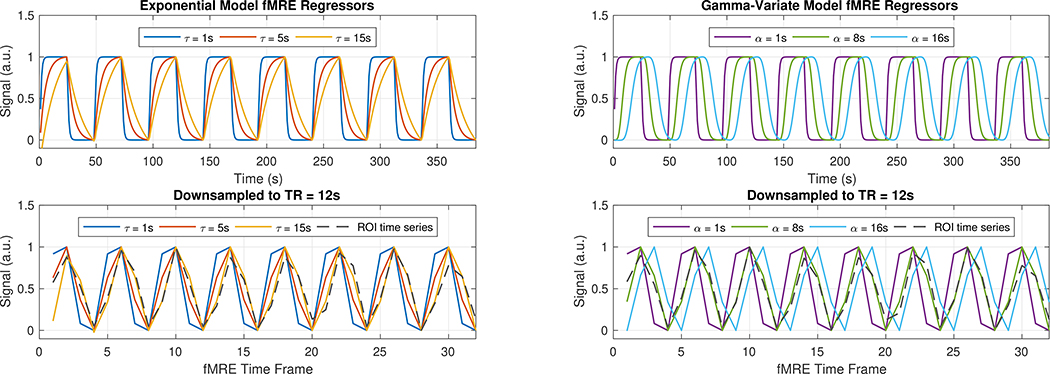
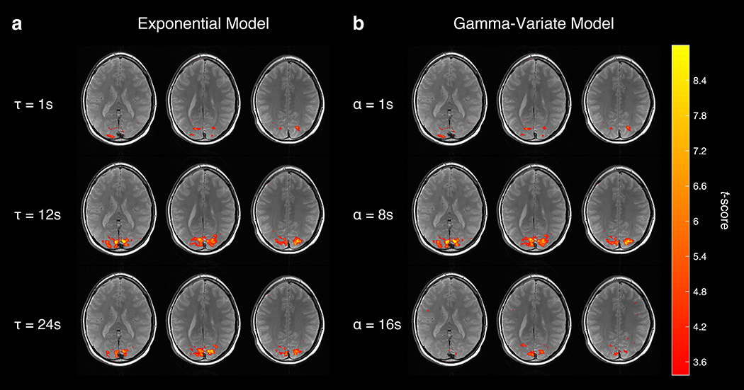
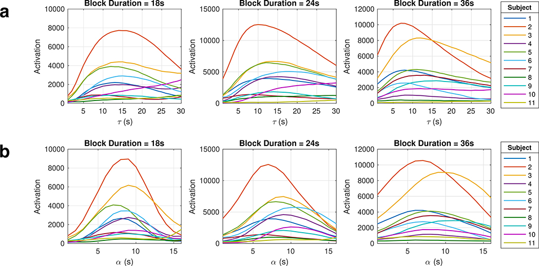
Initially, we analyzed the data with a one-sample t-test, essentially using a boxcar, or square wave, function as the regressor in a GLM analysis expecting rapid response [29]. However, the time series of the activated region of interest (ROI) followed more of a sawtooth pattern (Fig. 3, gray dashed curve), suggesting that the observed viscoelastic responses are occurring on a slower time scale. In Fig. 3, the ROI VE signal time course follows the regressor with a longer exponential time constant of τ = 15 s than it does the regressor with a shorter time constant of τ = 1 s. It also follows the regressor with the larger shape parameter α = 8 s than it does the regressor with a smaller α = 1 s. Plotting the activation maps as a function of model parameters τ and α demonstrates qualitatively greater activation, as defined in our previous methods section, when τ ≈ 12 s and when α ≈ 8 s (Fig. 4).

FIGURE 3.

(Top) Example of fMRE task regressors with varying time constants τ (Left) and shape parameters α (Right). (Bottom) Regressors downsampled to 12-s resolution, together with an empirically measured ROI time series (gray-dashed curve). Heuristically, the measurement correlates more with the regressors with the longer τ = 15 s and α = 8 s than with the shorter τ and α regressors.

FIGURE 4.

Example of a subject’s fMRE activation (p < 0.001) as a function of time constant τ (a) and gamma-variate shape parameter α (b). Notice that activation peaks near τ ≈ 12 s and α ≈ 8 s.

To further quantify the viscoelastic time constant, we plotted the activation versus the τ and α used in the first-order exponential decay model and gamma-variate model, respectively (Fig. 5). The τ* and α* for each run with valid model fits are recorded in Table 1, where the τ* values ranged from 7 s to 18 s and the α* values ranged from 6 s to 11 s. The estimated parameter values for runs where the activation did not have a maximum (continuously increases with the model parameter) were not recorded. These runs tend to have lower activation and contributes noise to the model parameter estimation. Averaging across all subjects for each block duration, we obtain τ* = 13.5 s, 12.9 s, 10.3 s for block durations 18 s, 24 s, and 36 s, respectively. The same averaging for the gamma-variate model results in α* = 8.4 s, 8.4 s, and 7.5 s for the three block durations. Pooling all runs and averaging the model parameter estimates yields τ* = 12.1 ± 3.0 s and α* = 8.1 ± 1.4 s.

FIGURE 5.

Quantification of fMRE activation versus the regressor’s time constant τ (a) and shape parameter α (b) for each of the three block durations. The τ at which the peak of each curve occurs is the arg max of activation, τ*; similarly the α at which the peak of each curve occurs is recorded as the α*.

TABLE 1.

Table of τ* and α* values for each subject, thresholded at p < 0.001.

Model Parameter	1st-order Exponential τ* (s)			Gamma-variate α* (s)
Subjects	BD = 18 s	BD = 24 s	BD = 36 s	BD = 18 s	BD = 24 s	BD = 36 s
Subject 1	13	12	8	8	7	6
Subject 2	14	10	7	9	7	7
Subject 3	15	14	12	9	9	9
Subject 4	15	15	8	9	9	8
Subject 5	12	12	11	7	8	8
Subject 6	15	18	9	9	11	7
Subject 7	10	8	13	7	6	8
Subject 8	-	-	7	8	8	6
Subject 9	14	14	16	9	9	11
Subject 10	-	-	12	9	10	7
Subject 11	-	-	-	-	-	6
Mean	13.5	12.9	10.3	8.4	8.4	7.5
SD	1.8	3.1	3.0	0.8	1.5	1.5
Total	12.1±3.0			8.1±1.4

BD, block duration; SD, standard deviation.

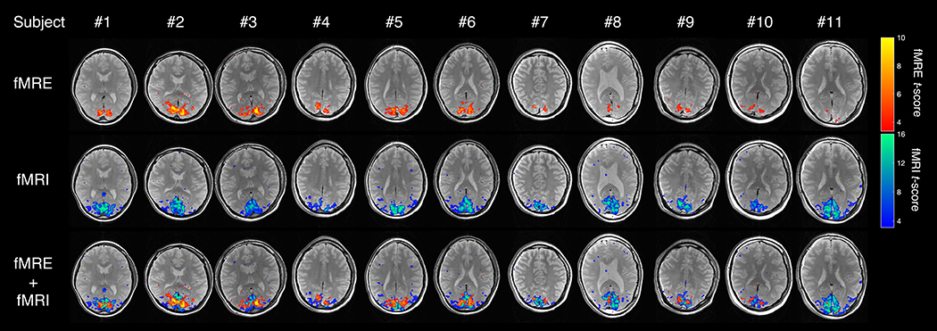
When averaged across all subjects, the fMRI activation ROI within the visual cortex had a stiffness value of 2.1±0.2 kPa. We were able to robustly detect significant stiffness changes in all 11 subjects’ V1 primary visual cortex region (Fig. 6). The increase in tissue stiffness due to visual activation was 6–11%, much larger than the increase in BOLD signal of 1–2% (Supplementary Table S1). The average percent signal change is 7.57±1.31% (Cohen’s d = 5.78) and 1.44±0.19% (Cohen’s d = 7.58) for fMRE and fMRI, respectively. The fMRE activation maps show spatially localized stiffness changes in the visual cortex, similar to the BOLD activation maps (Fig. 6). By overlaying the two activation maps, it is seen that the stiffness activation greatly colocalizes with the BOLD activation in the visual cortex. However, they are not exactly the same; a voxel-wise scatter plot of the fMRE t-scores versus fMRI t-scores also revealed no obvious relationship or trend (Supplementary Figure S1). While each point was considered activated in both fMRI and fMRE domains, the highest BOLD t-score did not necessarily correspond to the highest viscoelastic t-score. This is an interesting finding deserving further study beyond the scope of this paper.

FIGURE 6.

fMRE and fMRI t-score activation maps (p < 0.001) of the visual cortex for all 11 subjects; (top) stiffness-fMRE activation; (middle) BOLD-fMRI activation; (bottom) both fMRE (orange-yellow) and fMRI (blue-green) activation maps overlaid.

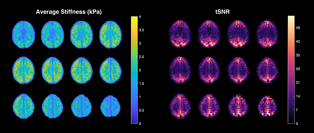
The average stiffness and temporal signal-to-noise ratio (tSNR_fMRE) maps derived from a subject’s fMRE time series are shown in Fig. 7. The average stiffness map depicts relatively uniform stiffness across the 12 brain slices, with a slight decrease in stiffness within the edge slices due to edge or boundary limitations of the stiffness calculations. The stiffness values are within the range of reported values in the literature [15]. However, the tSNR_fMRE maps are substantially more nonuniform than the stiffness, with the visual cortex having significantly higher tSNR_fMRE compared to other regions such as the auditory cortex. This is the result of spatially heterogeneous noise in the VE reconstruction, which could be caused by regional differences in the shear wave amplitude.

FIGURE 7.

The average stiffness (left) and temporal signal-to-noise ratio (tSNR_fMRE) (right) maps derived from a subject’s fMRE time series.

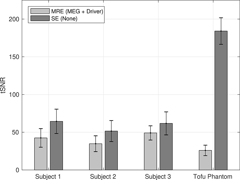
The effects of the MRE sequence and mechanical driver on the tSNR of the magnitude time series (tSNR_fMRI) in both the brain and the tofu phantom are shown in Fig. 8. Having both the MEGs and driver on (as during fMRE) results in more noise and lower tSNR_fMRI compared to having both turned off (as in during a conventional spin-echo sequence).

FIGURE 8.

Average tSNR_fMRI in the visual cortex for 3 subjects and a tofu phantom under 2 different conditions: (1) MEGs and driver, as in our MRE sequence; and (2) neither MEGs nor driver, as in a conventional spin echo sequence. The error bars indicate the standard deviation within the visual cortex. In all cases, the tSNR_fMRI of the SE sequence is greater than that of the MRE sequence (p < 0.001).

4 |. DISCUSSION

Our results provide convincing evidence that robust functional magnetic resonance elastography (fMRE) is possible in the human brain. Instead of performing a sham-controlled study like Patz et al., we used a time series method with alternating task and control blocks. As widely used in fMRI, this dynamical functional imaging method helps control for the effects of drift and changes in cognition over time. The incorporation of the time series method into fMRE allows firstly for robust activation maps on an individual basis, compared to previous methods that require the averaging over several individuals for significance [29]. Secondly, it also allows an estimate of the temporal characteristics of the VE changes, using a dictionary matching approach. The simultaneity of acquiring both BOLD and stiffness contrast is a third novel aspect introduced in this study. Both fMRE and fMRI detected regions with high effect sizes (Cohen’s d > 0.8), where d_fMRE = 5.78 and d_fMRI = 7.58. With simultaneous BOLD and stiffness activation maps, one can compare and contrast the neuromechanical and neurovascular coupling, which may provide richer understanding of the underlying neurobiology, especially while modulating other characteristics including physiological states such as vigilance.

Even though previous studies have indicated that MR elastography in the cortex is susceptible to partial-volume artifacts [40, 17], the partial-volume effects remain constant between frames in this study. However, the smoothness of the elastograms due to filtering could potentially affect the spatial localization of the fMRE activation.

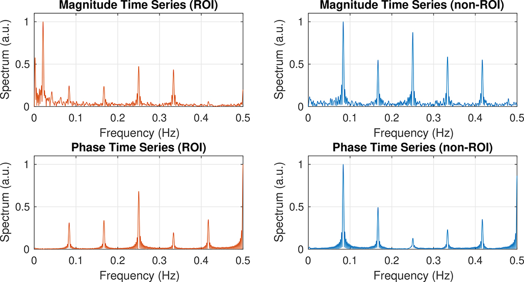
The magnitude and phase of the time series of the experiments yield mostly separate information —the magnitude information is indicative of T₂-weighted BOLD signal changes, whereas the phase information is used to generate the wave images and reconstruct the stiffness images. Because the MRE sequence used is a spin-echo EPI sequence, the BOLD contrast is localized to microvasculature and sensitive to dynamic averaging effects from water diffusion, thus more closely reflecting the venous microvascular changes in capillaries. Such acquisitions do not incur BOLD-related phase changes when averaged on the voxel scale. To further verify this, we looked at the spectrum of the magnitude and phase time series of an activated ROI versus a non-activated ROI (Fig. 9). As expected, the task frequency peak (0.021 Hz) only appears in the magnitude time series of the activated voxel and does not affect the phase information. Furthermore, the imaging sequence is both 0th- and 1st- gradient-moment-nulled; hence, it is flow-compensated and further prohibits fMRI BOLD effects from contaminating the MRE reconstructions.

FIGURE 9.

Frequency spectrum plots calculated from the magnitude (Top) and phase (Bottom) information of the spin-echo time series, with the DC term removed. (Left) Spectrum of an activated ROI (visual cortex) from an experiment with a 24-s block duration. (Right) Spectrum of a non-activated ROI from the same experiment. Notice that there is a peak at the task frequency of 0.021 Hz (48 s period) in the spectrum of the magnitude time series, but in none of the other panels. The peaks at other frequencies are due to the interaction between the motion-encoding gradients and phase offsets.

Similar to Patz et al.’s study, stiffness changes in the visual cortex were more significant in the real part of the complex shear modulus (G′ or storage modulus) than in the imaginary part (G″ or loss modulus) as shown in Supplementary Figure S2. This suggests that potential mechanisms for the observed neuromechanical coupling must affect mainly the elastic and less so the viscous processes. However, this could also be due to the fact that G″ has a proportionally larger variance compared to G′ due to its smaller magnitude. As shown in Supplementary Table S2, the storage modulus is much larger than the loss modulus in all subjects, meaning that the human brain is more elastic than dissipative.

The focus of our study was to achieve robust fMRE activation statistics on an individual subject basis per experiment, rather than to look for rapid mechanical changes that surpass BOLD frequencies as in [29]. The block durations we used —18 s, 24 s, and 36 s —were chosen due to our fMRE TR of 12 s per volume. Therefore, we observed temporal dynamics with first order time constants of 7 to 18 seconds and gamma-variate shape parameter of 6 to 11 seconds. At these slow time scales, the task ON states are stiffer than the task OFF states, unlike in the fast temporal dynamics regime as shown in Patz et al.’s study [29]. A potential explanation for the temporal increase in human brain stiffness while conducting functional tasks in this slow regime is the “garden hose effect,” where the increased perfusion pressure could stiffen the tissue, just as increased water pressure in a hose stiffens the flexible hose [41]. This is supported by the small but present increase in the loss modulus during task, as shown in Supplementary Figure S2. Another explanation for the observed increase in viscosity with task is the Fåhræus-Lindqvist effect, which describes how blood viscosity increases with an increase in capillary radius. As reported by Hetzer et al., hypercapnia-induced vasodilation and perfusion yields an increase in brain viscoelasticity (both stiffness and viscosity). Furthermore, cerebral blood flow (CBF) changes are correlated with viscosity changes but not stiffness changes [42].

Considering fMRI and fMRE contrast mechanisms, BOLD response is the result of coupling between cerebral blood flow (CBF), cerebral blood volume (CBV) and oxygen metabolism (CMRO2) [43]. The local deoxyhemoglobin concentration, which determines BOLD contrast, decreases in response to an increase in cerebral blood flow (CBF), but increases in response to an increase in venous blood volume (CBVv) or oxygen metabolism (CMRO2). Recent advances in arterial spin labeling (ASL) methods have allowed for the untangling of these physiolgoical processes that link neuronal signaling to the BOLD signal. Results from Simon et al. suggest relatively close coupling between metabolic and blood flow response and a much slower venous blood volume response [44]. This increase in blood flow with a lag in blood volume response can lead to an increase in perfusion pressure. Previous MRE studies have shown that an increase in perfusion pressure can lead to an increase in effective stiffness of in vivo brain [17, 42] and liver [45], whereas an occlusion of the renal artery that leads to decreased perfusion can lead to decreased tissue stiffness in the kidney [45]. Hence, in a way, the neuromechanical coupling effect we see may be tightly linked to the neurovascular coupling effect, just observed with changes in mechanical properties rather than blood oxygenation levels.

The two MRE elements (MEGs, passive driver) added to a spin-echo sequence were found to both contribute to a reduction in the tSNR of the magnitude time series (tSNR_fMRI, Fig. 8), most likely because of added subtle head motion or intravoxel phase dispersion from the shear wave motion [46]. Further study of this phenomenon is warranted.

Since the subjects of our study were healthy volunteers with minimal head motion (significantly less than the voxel size of 3 mm), separate motion correction on the reconstructed stiffness time series using downsampled motion parameters estimated by MCFLIRT from the fMRI magnitude time series was sufficient. For future studies, a more complete approach to motion correction for the fMRE time series would be to apply the transformation matrices estimated by MCFLIRT from the magnitude time series directly to the raw complex time series, preceding stiffness reconstruction.

Using an fMRE time series method opens the door to more robust fMRE studies and allows for characterization of various aspects of MRE signal and noise properties, such as in Figs. 7 and 8. Further work can explore whether tSNR_fMRE is adequate to allow fMRE in other regions of the brain, perhaps by modification of the wave generation methods. We have attempted fMRE with an auditory stimulus but were unable to detect significant activation (Supplementary Figure S3). This could be due to the large amount of time series noise in the auditory cortex during MRE. Furthermore, the fMRI activation itself was not very strong, perhaps due to the very loud motion encoding gradients from the background, which decreases the contrast between the ON and OFF blocks of auditory stimulus. In our sensory-motor task, there was also a passive motor task using plungers that move the fingers. Interestingly, weak fMRE activation was observed in the cerebellum, where the tSNR_fMRE is comparable to that in the primary visual cortex. Further work needs to be done for robust detection of sensory-motor activation.

Another interesting direction for future study would be to combine this method with the interleaved paradigm method, such that higher temporal dynamics of mechanical changes can be observed while also recording the BOLD signal evolution. This could potentially lead to deeper understanding of the separate contributions of stiffness changes due to functional tasks, e.g. nerve fibers swelling [47], aquaporins transporting water [48], and dendritic spines contracting [49] in response to stimulation.

In this study, the exponential model time constant τ*s demonstrate a trend towards reduction with longer block durations, although the variation is within standard deviation for the different block durations used in the visual task paradigm (Table 1). This trend suggested that the exponential VRF was not an optimal fit for the corpus of measurements, and we sought a better model. It was found that the gamma-variate model with a single parameter value fit measured activation results with less dependence on the block durations, which is therefore preferable. However, higher sampling rates (shorter TR_fMRE) might lead to a more complex model than our gamma-variate VRF.

Finally, the intersubject variation in stiffness values and percent fMRE signal fluctuation, along with the intersubject variation in τ* and α*, reflects biodiversity. As summarized by the brain MRE review by Hiscox et al., there is growing evidence in the literature relating individual differences in age, sex, cognition, etc. to brain stiffness. Whether factors such as age, sex, brain stiffness, cognition, etc. can affect fMRE activation should be a subject of further study.

5 |. CONCLUSION

In this study, we demonstrated that (1) very robust fMRE activation can be obtained using a novel time series method; (2) there are stiffness changes within the brain occurring on a slow time scale; (3) concurrent fMRE and fMRI is possible; (4) fMRE and fMRI activation maps strongly overlap within the visual cortex, and (5) the tSNR_fMRE is highly heterogenous in our study. This opens up the possibility of a new form of multi-modal brain mapping in the human cortex using two widely different contrast mechanisms. The integration of both hemodynamic and viscoelastic signals may provide complementary information useful for a deeper understanding of the underlying cognitive neurobiology mechanisms. Currently, our conclusions are limited to a visual task and a relatively small sample size; however, we hope these results will stimulate further exploration of fMRE.

Abbreviations

fMRI

functional magnetic resonance imaging

fMRE

functional magnetic resonance elastography

REFERENCES

- [1].Ogawa S, Lee TM, Kay AR, Tank DW. Brain magnetic resonance imaging with contrast dependent on blood oxygenation. Proc Natl Acad Sci U S A 1990;87(24):9868–72. https://www.ncbi.nlm.nih.gov/pubmed/2124706. [DOI] [PMC free article] [PubMed] [Google Scholar]
- [2].Muthupillai R, Lomas DJ, Rossman PJ, Greenleaf JF, Manduca A, Ehman RL. Magnetic resonance elastography by direct visualization of propagating acoustic strain waves. Science 1995;269(5232):1854–7. https://www.ncbi.nlm.nih.gov/pubmed/7569924. [DOI] [PubMed] [Google Scholar]
- [3].Mariappan YK, Glaser KJ, Ehman RL. Magnetic resonance elastography: a review. Clin Anat 2010;23(5):497–511. https://www.ncbi.nlm.nih.gov/pubmed/20544947. [DOI] [PMC free article] [PubMed] [Google Scholar]
- [4].Fovargue D, Nordsletten D, Sinkus R. Stiffness reconstruction methods for MR elastography. NMR Biomed 2018;31(10):e3935 https://www.ncbi.nlm.nih.gov/pubmed/29774974. [DOI] [PMC free article] [PubMed] [Google Scholar]
- [5].Manduca A, Oliphant TE, Dresner MA, Mahowald JL, Kruse SA, Amromin E, et al. Magnetic resonance elastography: non-invasive mapping of tissue elasticity. Med Image Anal 2001;5(4):237–54. https://www.ncbi.nlm.nih.gov/pubmed/11731304. [DOI] [PubMed] [Google Scholar]
- [6].Venkatesh SK, Yin M, Ehman RL. Magnetic resonance elastography of liver: technique, analysis, and clinical applications. J Magn Reson Imaging 2013;37(3):544–55. https://www.ncbi.nlm.nih.gov/pubmed/23423795. [DOI] [PMC free article] [PubMed] [Google Scholar]
- [7].Chen J, Yin M, Glaser KJ, Talwalkar JA, Ehman RL. MR Elastography of Liver Disease: State of the Art. Appl Radiol 2013;42(4):5–12. https://www.ncbi.nlm.nih.gov/pubmed/26366024. [PMC free article] [PubMed] [Google Scholar]
- [8].Chang W, Lee JM, Yoon JH, Han JK, Choi BI, Lee KB, et al. Liver Fibrosis Staging with MR Elastography: Comparison of Diagnostic Performance between Patients with Chronic Hepatitis B and Those with Other Etiologic Causes. Radiology 2016;280(1):88–97. https://www.ncbi.nlm.nih.gov/pubmed/26844364. [DOI] [PubMed] [Google Scholar]
- [9].Korsmo MJ, Ebrahimi B, Eirin A, Woollard JR, Krier JD, Crane JA, et al. Magnetic resonance elastography noninvasively detects in vivo renal medullary fibrosis secondary to swine renal artery stenosis. Invest Radiol 2013;48(2):61–8. https://www.ncbi.nlm.nih.gov/pubmed/23262789. [DOI] [PMC free article] [PubMed] [Google Scholar]
- [10].Low G, Owen NE, Joubert I, Patterson AJ, Graves MJ, Glaser KJ, et al. Reliability of magnetic resonance elastography using multislice two-dimensional spin-echo echo-planar imaging (SE-EPI) and three-dimensional inversion reconstruction for assessing renal stiffness. J Magn Reson Imaging 2015;42(3):844–50. https://www.ncbi.nlm.nih.gov/pubmed/25537823. [DOI] [PMC free article] [PubMed] [Google Scholar]
- [11].Hawley JR, Kalra P, Mo X, Raterman B, Yee LD, Kolipaka A. Quantification of breast stiffness using MR elastography at 3 Tesla with a soft sternal driver: A reproducibility study. J Magn Reson Imaging 2017;45(5):1379–1384. https://www.ncbi.nlm.nih.gov/pubmed/27779802. [DOI] [PMC free article] [PubMed] [Google Scholar]
- [12].Pepin KM, Ehman RL, McGee KP. Magnetic resonance elastography (MRE) in cancer: Technique, analysis, and applications. Prog Nucl Magn Reson Spectrosc 2015;90–91:32–48. https://www.ncbi.nlm.nih.gov/pubmed/26592944. [DOI] [PMC free article] [PubMed] [Google Scholar]
- [13].Bohte AE, Nelissen JL, Runge JH, Holub O, Lambert SA, de Graaf L, et al. Breast magnetic resonance elastography: a review of clinical work and future perspectives. NMR Biomed 2018;31(10):e3932 https://www.ncbi.nlm.nih.gov/pubmed/29846986. [DOI] [PubMed] [Google Scholar]
- [14].Dresner MA, Rose GH, Rossman PJ, Muthupillai R, Manduca A, Ehman RL. Magnetic resonance elastography of skeletal muscle. J Magn Reson Imaging 2001;13(2):269–76. https://www.ncbi.nlm.nih.gov/pubmed/11169834. [DOI] [PubMed] [Google Scholar]
- [15].Hiscox LV, Johnson CL, Barnhill E, McGarry MD, Huston J, van Beek EJ, et al. Magnetic resonance elastography (MRE) of the human brain: technique, findings and clinical applications. Phys Med Biol 2016;61(24):R401–R437. https://www.ncbi.nlm.nih.gov/pubmed/27845941. [DOI] [PubMed] [Google Scholar]
- [16].Murphy MC, Huston J, Ehman RL. MR elastography of the brain and its application in neurological diseases. Neuroimage 2019;187:176–183. https://www.ncbi.nlm.nih.gov/pubmed/28993232. [DOI] [PMC free article] [PubMed] [Google Scholar]
- [17].Hetzer S, Birr P, Fehlner A, Hirsch S, Dittmann F, Barnhill E, et al. Perfusion alters stiffness of deep gray matter. J Cereb Blood Flow Metab 2018;38(1):116–125. https://www.ncbi.nlm.nih.gov/pubmed/28151092. [DOI] [PMC free article] [PubMed] [Google Scholar]
- [18].Arani A, Murphy MC, Glaser KJ, Manduca A, Lake DS, Kruse SA, et al. Measuring the effects of aging and sex on regional brain stiffness with MR elastography in healthy older adults. Neuroimage 2015;111:59–64. https://www.ncbi.nlm.nih.gov/pubmed/25698157. [DOI] [PMC free article] [PubMed] [Google Scholar]
- [19].Sack I, Beierbach B, Wuerfel J, Klatt D, Hamhaber U, Papazoglou S, et al. The impact of aging and gender on brain viscoelasticity. Neuroimage 2009;46(3):652–7. https://www.ncbi.nlm.nih.gov/pubmed/19281851. [DOI] [PubMed] [Google Scholar]
- [20].Wuerfel J, Paul F, Beierbach B, Hamhaber U, Klatt D, Papazoglou S, et al. MR-elastography reveals degradation of tissue integrity in multiple sclerosis. Neuroimage 2010;49(3):2520–5. https://www.ncbi.nlm.nih.gov/pubmed/19539039. [DOI] [PubMed] [Google Scholar]
- [21].Streitberger KJ, Sack I, Krefting D, Pfüller C, Braun J, Paul F, et al. Brain viscoelasticity alteration in chronic-progressive multiple sclerosis. PLoS One 2012;7(1):e29888 https://www.ncbi.nlm.nih.gov/pubmed/22276134. [DOI] [PMC free article] [PubMed] [Google Scholar]
- [22].Murphy MC, Huston J, Jack CR, Glaser KJ, Manduca A, Felmlee JP, et al. Decreased brain stiffness in Alzheimer’s disease determined by magnetic resonance elastography. J Magn Reson Imaging 2011;34(3):494–8. https://www.ncbi.nlm.nih.gov/pubmed/21751286. [DOI] [PMC free article] [PubMed] [Google Scholar]
- [23].Fehlner A, Hirsch S, Guo J, Braun J, Sack I. The viscoelastic response of the human brain to functional activation detected by magnetic resonance elastography. ISMRM 22nd Annual Meeting 2014;p. 0871. [Google Scholar]
- [24].Holub O, Lambert SA, Schregel K, Bilston LE, Patz S, Sinkus R. Finger tapping experiment observed by brain Magnetic Resonance Elastography. ISMRM 23rd Annual Meeting 2015;p. 2530. [Google Scholar]
- [25].Patz S, Schregel K, Muradyan I, Kyriazis A, Wuerfel J, Mukundan S, et al. Observation of Functional Magnetic Resonance Elastography (fMRE) in Mouse Brain. ISMRM 23rd Annual Meeting 2015;p. 2526. [Google Scholar]
- [26].Patz S, Nazari N, Barbone PE, Fabry B, Fovargue D, Nordsletten D, et al. Functional Neuroimaging in the Brain using Magnetic Resonance Elastography. ISMRM 25th Annual Meeting 2017;p. 242. [Google Scholar]
- [27].Patz S, Fovargue D, Schregel K, Nazari N, Palotai M, Barbone PE, et al. Mapping Neural Circuitry at High Speed (10Hz) using functional Magnetic Resonance Elastography (fMRE). ISMRM 26th Annual Meeting 2018;p. 704. [Google Scholar]
- [28].de Arcos J, Fovargue D, Schregel K, Neji R, Patz S, Sinkus R. Imaging Primary Neuronal Activity in the Human Optical Cortex at 1.35Hz. ISMRM 26th Annual Meeting 2018;p. 147. [Google Scholar]
- [29].Patz S, Fovargue D, Schregel K, Nazari N, Palotai M, Barbone PE, et al. Imaging localized neuronal activity at fast time scales through biomechanics. Sci Adv 2019;5(4):eaav3816 https://www.ncbi.nlm.nih.gov/pubmed/31001585. [DOI] [PMC free article] [PubMed] [Google Scholar]
- [30].Ma D, Gulani V, Seiberlich N, Liu K, Sunshine JL, Duerk JL, et al. Magnetic resonance fingerprinting. Nature 2013;495(7440):187–92. https://www.ncbi.nlm.nih.gov/pubmed/23486058. [DOI] [PMC free article] [PubMed] [Google Scholar]
- [31].Poline JB, Brett M. The general linear model and fMRI: does love last forever? Neuroimage 2012;62(2):871–80. https://www.ncbi.nlm.nih.gov/pubmed/22343127. [DOI] [PubMed] [Google Scholar]
- [32].Glover GH. Deconvolution of impulse response in event-related BOLD fMRI. Neuroimage 1999;9(4):416–29. https://www.ncbi.nlm.nih.gov/pubmed/10191170. [DOI] [PubMed] [Google Scholar]
- [33].Guenthner C, Runge JH, Sinkus R, Kozerke S. Analysis and improvement of motion encoding in magnetic resonance elastography. NMR Biomed 2018;31(5):e3908 https://www.ncbi.nlm.nih.gov/pubmed/29601114. [DOI] [PMC free article] [PubMed] [Google Scholar]
- [34].Jenkinson M, Beckmann CF, Behrens TE, Woolrich MW, Smith SM. FSL. Neuroimage 2012;62(2):782–90. https://www.ncbi.nlm.nih.gov/pubmed/21979382. [DOI] [PubMed] [Google Scholar]
- [35].Woolrich MW, Ripley BD, Brady M, Smith SM. Temporal autocorrelation in univariate linear modeling of FMRI data. Neuroimage 2001;14(6):1370–86. https://www.ncbi.nlm.nih.gov/pubmed/11707093. [DOI] [PubMed] [Google Scholar]
- [36].Jenkinson M, Bannister P, Brady M, Smith S. Improved optimization for the robust and accurate linear registration and motion correction of brain images. Neuroimage 2002;17(2):825–41. https://www.ncbi.nlm.nih.gov/pubmed/12377157. [DOI] [PubMed] [Google Scholar]
- [37].Smith SM. Fast robust automated brain extraction. Hum Brain Mapp 2002;17(3):143–55. https://www.ncbi.nlm.nih.gov/pubmed/12391568. [DOI] [PMC free article] [PubMed] [Google Scholar]
- [38].Parker KJ. A microchannel flow model for soft tissue elasticity. Phys Med Biol 2014;59(15):4443–57. https://www.ncbi.nlm.nih.gov/pubmed/25049224. [DOI] [PubMed] [Google Scholar]
- [39].Parker KJ. Are rapid changes in brain elasticity possible? Phys Med Biol 2017;62(18):7425–7439. https://www.ncbi.nlm.nih.gov/pubmed/28766505. [DOI] [PubMed] [Google Scholar]
- [40].Guo J, Hirsch S, Fehlner A, Papazoglou S, Scheel M, Braun J, et al. Towards an elastographic atlas of brain anatomy. PLoS One 2013;8(8):e71807 https://www.ncbi.nlm.nih.gov/pubmed/23977148. [DOI] [PMC free article] [PubMed] [Google Scholar]
- [41].Bilston LE. Soft tissue rheology and its implications for elastography: Challenges and opportunities. NMR Biomed 2018;31(10):e3832 https://www.ncbi.nlm.nih.gov/pubmed/28991387. [DOI] [PubMed] [Google Scholar]
- [42].Hetzer S, Dittmann F, Bormann K, Hirsch S, Lipp A, Wang DJ, et al. Hypercapnia increases brain viscoelasticity. J Cereb Blood Flow Metab 2018;p. 271678X18799241 https://www.ncbi.nlm.nih.gov/pubmed/30182788. [DOI] [PMC free article] [PubMed] [Google Scholar]
- [43].Buxton RB, Wong EC, Frank LR. Dynamics of blood flow and oxygenation changes during brain activation: the balloon model. Magn Reson Med 1998;39(6):855–64. https://www.ncbi.nlm.nih.gov/pubmed/9621908. [DOI] [PubMed] [Google Scholar]
- [44].Simon AB, Buxton RB. Understanding the dynamic relationship between cerebral blood flow and the BOLD signal: Implications for quantitative functional MRI. Neuroimage 2015;116:158–67. https://www.ncbi.nlm.nih.gov/pubmed/25862267. [DOI] [PMC free article] [PubMed] [Google Scholar]
- [45].Yin M, Glaser KJ, Kolipaka A, Warner L, Talwalkar JA, Manduca A, et al. Influence of Perfusion on Tissue Stiffness Assessed with MR Elastography. ISMRM 18th Annual Meeting 2010;p. 256. [Google Scholar]
- [46].Glaser KJ, Felmlee JP, Manduca A, Ehman RL. Shear stiffness estimation using intravoxel phase dispersion in magnetic resonance elastography. Magn Reson Med 2003;50(6):1256–65. https://www.ncbi.nlm.nih.gov/pubmed/14648574. [DOI] [PubMed] [Google Scholar]
- [47].Iwasa K, Tasaki I, Gibbons RC. Swelling of nerve fibers associated with action potentials. Science 1980;210(4467):338–9. https://www.ncbi.nlm.nih.gov/pubmed/7423196. [DOI] [PubMed] [Google Scholar]
- [48].Papadopoulos MC, Verkman AS. Aquaporin water channels in the nervous system. Nat Rev Neurosci 2013;14(4):265–77. https://www.ncbi.nlm.nih.gov/pubmed/23481483. [DOI] [PMC free article] [PubMed] [Google Scholar]
- [49].Korkotian E, Segal M. Spike-associated fast contraction of dendritic spines in cultured hippocampal neurons. Neuron 2001;30(3):751–8. https://www.ncbi.nlm.nih.gov/pubmed/11430808. [DOI] [PubMed] [Google Scholar]
Associated Data
This section collects any data citations, data availability statements, or supplementary materials included in this article.