

Abstract
Previous studies have focused on changes in the geographical distribution of terrestrial biomes and species targeted by marine capture fisheries due to climate change impacts. Given mariculture's substantial contribution to global seafood production and its growing significance in recent decades, it is essential to evaluate the effects of climate change on mariculture and their socio‐economic consequences. Here, we projected climate change impacts on the marine aquaculture diversity for 85 of the currently most commonly farmed fish and invertebrate species in the world's coastal and/or open ocean areas. Results of ensemble projections from three Earth system models and three species distribution models show that climate change may lead to a substantial redistribution of mariculture species richness potential, with an average of 10%–40% decline in the number of species being potentially suitable to be farmed in tropical to subtropical regions. In contrast, mariculture species richness potential is projected to increase by about 40% at higher latitudes under the ‘no mitigation policy’ scenario (RCP 8.5) by the mid‐21st century. In Exclusive Economic Zones where mariculture is currently undertaken, we projected an average future decline of 1.3% and 5% in mariculture species richness potential under RCP 2.6 (‘strong mitigation’) and RCP 8.5 scenarios, respectively, by the 2050s relative to the 2000s. Our findings highlight the opportunities and challenges for climate adaptation in the mariculture sector through the redistribution of farmed species and expansion of mariculture locations. Our results can help inform adaptation planning and governance mechanisms to minimize local environmental impacts and potential conflicts with other marine and coastal sectors in the future.
Keywords: aquaculture, climate change, habitat suitability, scenarios, seafood production
We analysed the impacts of climate change on global mariculture species richness for 85 of the currently most commonly farmed species by the 2050s relative to the 2005s. Results of ensemble projections show that climate change may lead to a substantial redistribution of mariculture species richness potential, with an average of 10%–40% decline in the number of species being potentially suitable to be farmed in tropical to subtropical regions. In contrast, potential mariculture species diversity is projected to increase by about 40% at higher latitudes under the ‘no mitigation policy’ scenario (RCP 8.5) scenario by the mid‐21st century.

1. INTRODUCTION
The world population is projected to reach an estimated 9–10 billion by 2050, increasing global food demand by 70%–100% (Alexandratos & Bruinsma, 2012; Baulcombe et al., 2009; De Silva & Soto, 2009; Kapetsky, Aguilar‐Manjarrez, & Jenness, 2013). Meeting the global food demand—and doing so in a way that limits environmental damage—is a fundamental challenge to sustainable development (UN, 2019). Between 2011 and 2015, marine capture fisheries and mariculture (both marine and brackish water aquaculture) produced an average 105.5 million tonnes of seafood annually (FAO, 2018). For approximately 3.2 billion people in the world, seafood contribute, about 20% of their protein intake (FAO, 2018). Compared to animal production on land, seafood is generally considered to have a lower environmental impact (Hilborn, Banobi, Hall, Pucylowski, & Walsworth, 2018)—yet the role of seafood in achieving the sustainable development goals remains under‐recognized and undervalued (HLPE, 2014). As a food high in protein and low in trans‐unsaturated fatty acids, seafood provides a range of positive health benefits. Seafood consumption is recommended in most dietary guidelines (Meyer et al., 2003) mainly because finfish and shellfish are an essential source of highly bioavailable vitamins, minerals and omega‐3 (n‐3) and omega‐6 (n‐6) polyunsaturated fatty acids (PUFAs; Larsen, Eilertsen, & Elvevoll, 2011; Tocher, 2015). The latter is important notably for cardiovascular health, cognitive function and prenatal and postnatal brain development (Giles, Mahoney, & Kanarek, 2019; Harris, Miller, Tighe, Davidson, & Schaefer, 2008; Innis, 2008).
Aquaculture has played an essential role in filling the gap between food fish (finfish, crustaceans, molluscs and other aquatic animals, but excluding seaweeds and products not for human consumption) demand and supply from capture fisheries. Global production of food fish from aquaculture (freshwater, marine and brackish) has increased from 2.6 million in 1970 to nearly half of the 171 million tonnes of food fish (excluding aquatic plants) consumed worldwide in 2016 (FAO, 2018); with Asia continuing to dominate the sector and accounting for more than 92% of global aquaculture production (Phillips & Pérez‐Ramírez, 2017). The contribution of mariculture (including brackish production) share in total aquaculture has increased markedly from 14% in 2000 to 37% in 2016 (FAO, 2018). Mariculture is a form of aquaculture where ‘cultivation of the end product takes place in seawater, such as fjords, inshore and open waters, and inland seas or inland facilities (Recirculating Aquaculture System, RAS) in which the salinity exceeds 20 PSU’ (FAO, 2004). The Sea Around Us mariculture database (http://www.searoundus.org) estimated an increase in mariculture production from 5 million tonnes in 1990 to 21 million tonnes in 2010. This increased production is primarily driven by the growing demand for seafood in developed countries (Campbell & Pauly, 2013; FAO, 2014), which focuses on high value omnivorous and carnivorous species (FAO, 2014). Although projections of the future contribution of aquaculture—including mariculture—to food supply is uncertain, it has been estimated that if all inputs were available, the sector could provide 16–47 million additional tonnes of fish by 2030 (Hall, Delaporte, Phillips, Beveridge, & O′Keefe., M., 2011). While aquaculture may increase food provision, it is important to note that recent work shows that from a nutritional perspective, species from capture fisheries, may provide a greater contribution to micronutrient intakes than common aquaculture species (Bogard et al., 2015).
Yet, climate change could reduce the anticipated potential seafood supply from mariculture. Sea level rise, increases in water temperature, ocean acidity, storm frequencies and wave action, as well as changes in salinity, among others, are expected to impact the suitability of marine habitats (coastal waters and open ocean) to farm seafood (Barange & Perry, 2009; Cheung et al., 2009; Gattuso et al., 2015; Harley et al., 2006). Increases in temperature and acidity, in particular, are also expected to directly affect the physiology and ecology of farmed species (Cochrane, Young, Soto, & Bahri, 2009) by altering growth rates, disease susceptibility, survival rates, reproduction and shell quality in the case of bivalves (Handisyde, Ross, Badjeck, & Allison, 2006). Such environmental changes might lead to a reduction in areas suitable for mariculture and redistribution of farmed species from their historical farming range—particularly for species that are farmed using open or semi‐open production systems, including salmon. Thus, climate change is expected to affect the quantity and quality of seafood production from mariculture. Two studies have estimated the areas currently not utilized, but potentially suitable for mariculture, which could increase seafood production to contribute to and improve food security in the future (Gentry et al., 2017; Oyinlola, Reygondeau, Wabnitz, Troell, & Cheung, 2018). However, these areas are likely to be impacted by climate change, thereby reducing the chances of mariculture expansion and associated projected production of seafood in the future.
Recent studies that investigated climate change effects on the growth potential and availability of suitable marine areas for mariculture (Froehlich, Gentry, & Halpern, 2018; Klinger, Levin, & Watson, 2017) suggest that climate change impact will be heterogeneous across species and regions. Noticeable adverse effects are projected for mariculture‐suitable marine areas around the equator with substantial gains towards the poles. Selective breeding (Klinger et al., 2017), risk‐based zoning and siting (Barange et al., 2018; Froehlich et al., 2018) and changes to alternative farm species with favourable growth rates and market acceptability (Harvey, Soto, Carolsfeld, Beveridge, & Bartley, 2016) have been suggested as potential adaptation strategies that could be important to increase seafood production from mariculture under climate change.
To date, climate change impacts on mariculture species richness or diversity remains poorly understood (Oyinlola et al., 2018). Here, mariculture species richness potential (MSRP) represents the total number of species that can be farmed given a set of specific environmental conditions. The suitability of the environments is dependent on biological factors (e.g. species environmental preferences and tolerances), socio‐economic (e.g. management restrictions) and technological factor (e.g. availability of technology to farm offshore; Oyinlola et al., 2018). Species richness relates to the potential for diversification of mariculture operation, which contributes to its sustainability (Harvey et al., 2016).
Species distribution models (SDMs) are numerical tools that link species occurrences in time and space with environmental conditions—and can, therefore, be used to predict species occurrences based on environmental data sets (Elith & Leathwick, 2009; Guisan & Zimmermann, 2000). Generally, SDMs generate a statistical or non‐parametric relationship between environmental conditions such as temperature, oxygen, salinity, pH and other ocean variables with species’ occurrences, which are then used to define their potential fundamental niche (Hutchinson, 1959). The models ultimately predict an index of habitat suitability for the species around the niche (Elith & Leathwick, 2009). These tools have been widely used to assess past, current and future distributions of terrestrial (Newbold, 2018; Polce et al., 2013) and marine species (Cheung, Brodeur, Okey, & Pauly, 2015; Cheung et al., 2010; Jones & Cheung, 2014) as well as to quantify the potential suitable marine areas for mariculture (Oyinlola et al., 2018).
In this study, we quantify global patterns of MSRP for 85 species identified as some of the currently most commonly farmed marine species in coastal and/or open ocean areas and project future trends and patterns under climate change. Specifically, we estimate a ‘mariculture diversity index’ for a given location and determine how it would change by the middle and end of the 21st century under strong mitigation and ‘no mitigation policy’ scenarios using an ensemble model approach with three Earth system models (ESMs) and three SDMs. We discuss the implications of our findings for future seafood production and the environmental and socio‐economic opportunities and challenges of climate adaptation for the mariculture sector.
2. MATERIALS AND METHODS
The method applied in this study includes five main steps. First, we quantified the historical mean ocean conditions (average of 1970–2000) suitable for farming aquatic organisms and estimated the environmental niche of 85 of the most commonly farmed species (Table S1). We then projected their habitat suitability index (HSI) over the global ocean based on average historical environmental conditions. We further estimated the future habitat suitability index for mariculture for each of the 85 currently most commonly farmed species under future scenarios of ocean conditions as determined by three ESMs. We calculated the changes in mariculture diversity based on the model projections and used the averaged outputs (average across ESMs by spatial cell) to assess the impacts of climate change on mariculture. Lastly, we quantified associated model uncertainties. Details of each step are provided below.
2.1. Occurrence data
We obtained occurrence records of mariculture farm locations within countries' Exclusive Economic Zones (EEZ) for 85 of the most commonly farmed marine species from the georeferenced mariculture database developed by and described in Oyinlola et al. (2018). The database was developed by obtaining the list of farmed species from the Sea Around Us global mariculture database (GMD; http://www.seaaroundus.org). We extracted the species’ names of all fish and invertebrates reported in the database (307 in total)—excluding all records not at the species level. Using all subnational units where farms are recorded in the GMD, we visually identified mariculture installations (i.e. tanks, pens, cages and lines) based on satellite imagery available from Google Earth (http://www.google.com/earth/). The coordinates of each installation were then extracted using the Google Earth placemark tool (Trujillo, Piroddi, & Jacquet, 2012). All species’ farm location records were converted to a binary of presence or absence and rasterized on a regular spatial grid of 0.5° latitude × 0.5° longitude over the global ocean.
We focused on these species because of their high economic and nutritional importance. Together, these species accounted for about 70% of all mariculture production out of 307 taxa farmed globally in 2015. These 85 species also met the minimum occurrence data requirements of more than seven subnational units for SDMs (Elith et al., 2006), that in turn allow greater model accuracy when projecting future changes. These species included 55 chordates and 30 molluscs.
2.2. Environmental data
We assembled data sets for eight environmental parameters: sea surface temperature, dissolved oxygen concentration, chlorophyll‐a concentration, salinity, pH, silicate concentration, current velocity and euphotic depth. We obtained 10‐year averaged ocean current velocity data (1992–2002) from Estimating the Circulation and Climate of the Ocean (ECCO) Project (http://www.ecco-group.org). We gathered values for temperature, pH, dissolved oxygen concentration, salinity, silicate concentration and chlorophyll‐a concentration (the latter two parameters are used as proxy for food source for molluscs; Newell, 2004; Oyinlola et al., 2018; Pilditch, Grant, & Bryan, 2001) from three ESMs that were part of the Coupled Models Inter‐comparison Project Phase 5 (CMIP5): (a) the Geophysical Fluid Dynamics Laboratory Earth System Model 2M (GFDLESM2M), (b) the Institute Pierre Simon Laplace coupled model version 5 (IPSL; IPSL‐CM5‐MR), and (c) the Max Planck Institute for Meteorology Earth System Model (MPI‐ESM‐MR) and averaged over the period 1970–2000 for each ESM. All environmental data were interpolated using bilinear methods (Legendre & Legendre, 2012) over the global ocean (189.75°W to 179.75°E and 89.75°N to 89.75°S) on a regular spatial grid of 0.5° latitude × 0.5° longitude (the same as occurrence rasterized data) and for two vertical layers: surface (0–10 m) and sea bottom depth, where available.
2.3. Habitat suitability index
We used a multispecies distribution model approach to determine areas that would be considered as suitable for farming the 85 selected species. First, we harmonized the coordinates of the rasterized farm location data and environmental data on a regular spatial grid of 0.5° × 0.5° and determined the environmental quality parameters that best explain the occurrences of farming locations using the eigenvalue diagram (Oyinlola et al., 2018) implemented in the Ecological Niche Factor Analysis (ENFA; Basille, Calenge, Marboutin, Andersen, & Gaillard, 2008). The diagram was constructed based on the departure of the ecological niche from the mean habitat for each species, thus identifying the species’ preference for particular environmental parameters among the whole set of parameters. We selected the essential collection of environmental parameters by determining the direction where ‘specialization’ is highest. The specialization is a measure of the narrowness of the niche; in other words, the higher the specialization, the more restricted the niche. These selected environmental parameters represent the essential water physio‐chemical parameters needed for farming each species and are used in predicting the habitat suitability index of the SDMs.
We then computed current MSRP using three SDMs: Gradient Boosting Machine (GBM; Ayyadevara, 2018; Friedman, 2002), Surface Range Envelope (SRE; Busby, 1991) and Maximum Entropy (MAXENT; Phillips, Anderson, & Schapire, 2006). Next, we applied each model to estimate the habitat suitability index (HSI) of each species for each gridded cell of the ocean (i.e. 0.5° × 0.5°). The HSI scales from 0 to 1 (low to high) to indicate the environmental suitability of the selected environmental conditions for each species in each spatial cell.
2.4. Present suitable areas for mariculture
We identified an area as potentially suitable for mariculture based on the SDMs' results, and a set of additional environmental and socio‐economic constraints. First, by comparing the predicted HSI with current gridded farm location data, we determined the minimum HSI above which mariculture can potentially occur. The thresholds were identified at the species level by quantifying a species’ 'prevalence' (i.e. the fraction of cells in which the species is present; Phillips et al., 2009). We set the known farm locations' HSI as 'presence' and the locations with suitable HSI but no farms as 'absence' and evaluated 'prevalence' using the evaluate function in the R dismo package (Hijmans, Phillips, Leathwick, Elith, & Hijmans, 2017). The predictive values of habitat suitability for mariculture below the prevalence value were assigned 0 and predicted HSI values higher than the prevalence value were assigned 1. Second, we assumed that farm operations would not extend beyond a country's EEZ. Third, we assumed that mariculture activities would be restricted by currents and only included spatial cells with a current velocity between 10 cm/s and 100 cm/s (Kapetsky et al., 2013). Lastly, as most marine protected areas (MPAs) do not allow aquaculture, existing MPAs, as documented in the Atlas of Marine Protection (http://www.mpatlas.org/), were not considered as suitable areas for future marine aquaculture activities (Table 1).
Table 1.
Criteria for including marine area as suitable for mariculture production
| Criteria | Justification | Threshold |
|---|---|---|
| Habitat Suitability Index above the occurrence threshold | Exclude area with environmental conditions that are not suitable for the growth and survival of the farmed species |
‘Prevalence (pv)’ the fraction of cells at which the species is present (Phillips et al., 2009) HSI = 1, if HSI ≥ pv HSI = 0, if HSI < pv |
| Within the Exclusive Economic Zone | Political boundary | 200.0 nm (370.4 km) |
| Within a range of ocean current velocities | Mariculture operations avoid disturbance from strong ocean currents | Current velocity between 10 cm/s and 100 cm/s (Kapetsky et al., 2013) |
| Outside of designated marine protected areas | Most MPAs do not allow aquaculture operations within their boundaries | Exclude designated marine protected areas |
2.5. Model testing
We tested the robustness of the SDM outputs by comparing the predicted HSI with reference records of species occurrences. We ran the model with 75% of all records as a training data set to develop each SDM and calculate each species’ HSI. The remaining 25% of the data were used for model evaluation. The Area Under the Receiver Operating Characteristic Curve (AUC) for each set of model predictions was calculated using the ROCR package in R (Sing, Sander, Beerenwinkel, & Lengauer, 2005). AUC values range from 0 to 1, with 0.5 indicating that the model is no better than a random sample of values, and 1 indicating that the model has high predictive power. The individual species model was then used as weighting values for the multimodel ensemble (Jones & Cheung, 2014).
2.6. Projection of future suitability index
Model projections for the future suitability of the ocean for farming of the 85 species included in this study under climate change were run using outputs from three ESMs in CMIP5: GFDL‐ESM‐2M; IPSL‐CM5‐MR and MPI‐ESM‐MR. Two climate change scenarios were considered: Representative Concentration Pathway (RCP) 2.6 and RCP 8.5, commonly referred to as the ‘strong mitigation’ and ‘no mitigation policy’ greenhouse gas emission scenarios respectively. We present the individual ESM output and the multimodel output (average across ESM models by spatial cell).
2.7. Analysis
We analysed the global pattern of change in MSRP from 1995 to 2100 under the two climate change scenarios. We estimated the MSRP in each 0.5° × 0.5° cell and then calculated the total number of species that could be potentially farmed in each EEZ for the 85 selected species for each year from 1995 to 2100. We then estimated the global and regional percentage change in MSRP in the 2000s (i.e. an average of 1995–2015), the 2050s (i.e. an average of 2040–2060) and the 2090s (i.e. an average of 2080–2100). Percentage change in MSRP was estimated for all potential mariculture countries, countries with currently existing mariculture activities and at the species level. Using model outputs, we discuss the potential opportunities and challenges for the future sustainable development of global mariculture. All models and analyses were run using the statistical programming software R (R Core Team, 2018) and maps were made in Matlab (MATLAB and Statistics Toolbox Release 2018b, 2018).
3. RESULTS
3.1. Model evaluation
All three models estimate distributions of MSRP that are strongly supported by observations, as indicated by the high AUC model values (Figure S1). The AUC values varied among ESMs and SDMs, with the 25th and 75th percentiles of Surface Range Envelope (SRE; Average AUC across all ESM models) predictions having AUC values of 0.76 and 0.91 across models respectively (an AUC value of 0.5 indicates that a model's prediction is no better than random choice). Maximum Entropy (MAXENT) and Gradient Boosting Machine (GBM) had the highest AUC values; with both scoring AUC values of 0.91 and 0.95 for the 25th and 75th percentiles, respectively. The 25th and 75th percentiles of the estimated prevalence value for each species (i.e. the HSI threshold below which the marine area was considered unsuitable for culturing the specific modelled species) ranged from 0.32 to 0.65.
3.2. Current mariculture richness and potentially suitable marine area for mariculture
Our model predicted the current pattern of MSRP across all models for the reference time (2000s, average between 1995 and 2015) under the strong mitigation RCP 2.6 and ‘no mitigation policy’ scenarios RCP 8.5 (Figure 1a). Results show similar trends under both scenarios. MSRP was highest in the north subtropics (66.5°N and 35.5°N; Figure 1b), particularly the East China Sea (species richness = 25–53 across RCP scenarios) and north of the Gulf of Mexico (species richness = 15–45 across RCP scenarios). Lowest MSRP was estimated for the North Frigid Zone (i.e. Arctic; 90°N and 66.5°N). Other noticeable areas of richness include the southwestern Atlantic coast (species richness = 30–45 across RCP scenarios) and West Africa (species richness = 35–40 across RCP scenarios), the Yellow Sea (species richness = 30–50 across RCP scenarios) and the Caribbean Sea (species richness = 20–40 across RCP scenarios).
Figure 1.

Predicted global distribution and range of mariculture species richness potential (MSRP) for the reference period (1995–2015) for 85 species of finfish and molluscs under RCP 8.5 (a) on 0.5° by 0.5° grid cells, and (b) by latitude. Boxes in (b) represent the interquartile range of number of species; the horizontal lines in the boxplot represent median values, and the upper and lower whiskers represent scores outside the interquartile range. All results presented as a multimodel ensemble. Arctic (66.5°N to 90°N), north temperate (35.5°N to 66.5°N), north subtropics (23.5°N to 35.3°N), tropics (23.5°N to 23.5°S), south subtropics (23.5°S to 35.5°S) and south temperate (35.5°S to 66.5°S)
Also, under both scenarios (RCP 2.6 and 8.5), we estimated a total of 113 million km2 of suitable marine area for the mariculture of all 85 selected species in the 2000s (Figure 2), ranging at the regional level from 66 million km2 in the tropics to 7.8 million km2 in the Arctic. Total suitable area for finfish and molluscs was estimated at 83 million km2 and 49 million km2, respectively.
Figure 2.

Total estimated potential suitable mariculture area for 85 species at present (2000s, average between 1995 and 2015), 2050s (average between 2040 and 2060) and 2090s (average between 2080 and 2100). (a) Regional projection under RCP 2.6, (b) regional projection under RCP 8.5, (c) species group under RCP 2.6, (d) species group under RCP 8.5. Arctic circle (90°N and 66.5°N), north temperate (66.5°N and 35.5°N), north subtropics (35.3°N and 23.5°N), tropics (23.5°N and 23.5°S), south subtropics (23.5°S and 35.5°S) and south temperate (35.5°S and 66.5°S)
3.3. Climate change mediated impacts on mariculture species richness and potentially suitable marine mariculture areas
Relative to current (1995–2015) MSRP, projected future MSRP only changed slightly globally. Under RCP 2.6, the model ensemble projected an increase in MSRP of 1.02% ± 0.59 (standard error) by the 2050s (average between 2040 and 2060) and 3.35% ± 0.62 by the 2090s (average between 2080 and 2100; Table 2, Figure 3a). A decrease of 0.49% ± 0.11 was projected by the 2050s and an increase of 2.39% ± 0.53 by the 2090s under RCP 8.5 (Table 2, Figure 3b).
Table 2.
Percentage change in global mariculture species richness potential by mid‐century (average between 2040 and 2060) and end of the century (average between 2080 and 2100) relative to the 2000s (average between 1995 and 2015) under RCP 2.6 and RCP 8.5 scenarios
| Model uncertainty | ||||||||
|---|---|---|---|---|---|---|---|---|
| % Change in mariculture species richness potential | ||||||||
| GFDL | IPSL | MPI | Multimodel | |||||
| 2050s | 2090s | 2050s | 2090s | 2050s | 2090s | 2050s | 2090s | |
| RCP 2.6 (global) | 1.89 | 4.57 | −0.10 | 2.92 | 1.28 | 2.56 | 1.02 ± 0.59 | 3.35 ± 0.62 |
| RCP 8.5 (global) | −0.64 | 2.62 | −0.57 | 3.18 | −0.27 | 1.38 | −0.49 ± 0.11 | 2.39 ± 0.53 |
The error limits represent the standard deviation across Earth System Models.
Abbreviations: GFDL, Geophysical Fluid Dynamics Laboratory Earth System Model 2; IPSL, Institute Pierre Simon Laplace; MPI, Max Planck Institute for Meteorology Earth System Model.
Figure 3.
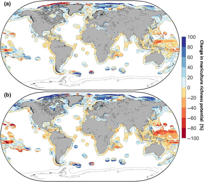
Impacts of climate change on global mariculture species richness potential for 85 of the currently most commonly farmed species by the 2050s (average 2040 and 2060) relative to the 2000s (average 1995 and 2015). The black line in the ocean represents the boundary of Exclusive Economic Zones (Sea Around Us, http://www.searoundus.org). Percentage changes under (a) RCP 2.6 and (b) RCP 8.5. Warm colours represent losses while cool colours represent gains
However, projected changes in MSRP under climate change showed important differences across latitudes (Figure 4a,b). The latitudinal average was projected to shift towards the poles (i.e. South and North) under the two RCP scenarios. Under RCP 2.6, MSRP in the tropics was found to decline by 2.23% ± 21.10 (standard deviation) by the 2050s relative to the 2000s, compared to a decline of 10.08% ± 25.72 under RCP 8.5 over the same time frame. An increase of about 19.69% ± 47.1 was observed between 90°N and 66.5°N under RCP 2.6 compared to a projected increase of 41.11% ± 42.19 under RCP 8.5, for the same time period.
Figure 4.

Latitudinal average of the mean percentage change in mariculture species richness potential in the 2050s compared to the 2000s under (a) RCP 2.6 and (b) RCP 8.5. Boxes represent the interquartile range of per cent changes; the horizontal lines in the boxplot represent median values, and the upper and lower whiskers represent scores outside the interquartile range. All results presented as a multimodel ensemble. Arctic circle (90°N and 66.5°N), north temperate (66.5°N and 35.5°N), north subtropics (35.3°N and 23.5°N), tropics (23.5°N and 23.5°S), south subtropics (23.5°S and 35.5°S) and south temperate (35.5°S and 66.5°S)
Under RCP 2.6, the model ensemble projected a decline of 1.42% ± 0.31 (standard deviation) in the marine area suitable for mariculture by the 2050s and 1.20% ± 0.26 by the 2090s (Figure 2a). A decline of 2.01% ± 0.52 and 3.69% ± 0.59 was projected by the 2050s and 2090s, respectively, under the RCP 8.5 scenario (Figure 2b). Similarly, global potentially suitable mariculture area was projected to decline by 1.95% ± 0.89 under RCP 2.6, and by 1.48% ± 0.72 under RCP 8.5 by the 2050s for finfish (Figure 2c). For molluscs, the total marine area potentially suitable for mariculture declined by 5.26% ± 3.29 and 6.36% ± 3.34 under RCP 2.6 and 8.5 respectively (Figure 2d).
3.4. Projected climate change impacts on the Exclusive Economic Zones with existing mariculture industry
Globally, the EEZs that currently have farm operations were projected to lose 1.26% ± 0.54 and 4.99% ± 0.12 in MSRP under RCP 2.6 and RCP 8.5, respectively, by mid‐century relative to the 2000s period (Table 3). These projections focused on EEZs where mariculture facilities are currently known to operate and where there is a historical record of farming a given species. Specifically, MSRP was projected to decline in about 62% of EEZs worldwide. Many countries with established mariculture operations since 1950 were projected to lose an important cultured marine species due to ocean parameters unsuitable for the relevant species by the middle of the century under both RCP 2.6 and RCP 8.5 (Figure 5a,b). We projected declines between 20% and 100% in currently utilized EEZs by mid‐century relative to the 2000s under both RCP 2.6 and 8.5 scenarios, respectively, in EEZs of the Pacific and Western Indian Ocean Small Island States and Territories, as well as Indonesia, Russia, Chile and Ecuador. Large declines (30%–70%) were also projected for Canada (Pacific coast; median 56.57%), southern Chile (median −39.54%), Senegal (median 45.29%) and the Philippines (median 63.87%). Specifically, the Pacific coast of Canada, southern Chile and the Philippines were projected to lose in finfish MSRP (Figure 6a). However, we projected a slight increase in molluscs’ MSRP (Figure 6b). Under RCP 8.5, moderate levels of decline (approximately 20%) were projected for the Caribbean Sea, and waters around Europe, Morocco, Japan and Australia. Increases in currently utilized EEZs for selected farmed species were projected for Newfoundland and Labrador in Canada (60%–70%), parts of Argentina's EEZ (10%–20%), around India (20%–80%), Turkey and Greece (5%–20%), Natal—Brazil (10%–60%) and the northern Philippines Sea (20%–100%).
Table 3.
Percentage change in mariculture species richness potential in Exclusive Economic Zones with currently established operations, for select species, by mid‐century (average between 2040 and 2060) and end of the century (average between 2080 and 2100) relative to the 2000s (average between 1995 and 2015) under RCP 2.6 and 8.5 scenarios
| Model uncertainty | ||||||||
|---|---|---|---|---|---|---|---|---|
| % Change in mariculture species richness potential | ||||||||
| GFDL | IPSL | MPI | Multimodel | |||||
| 2050s | 2090s | 2050s | 2090s | 2050s | 2090s | 2050s | 2090s | |
| RCP 2.6 (global) | −1.79 | −2.15 | −1.79 | −2.15 | −0.19 | −1.48 | −1.26 ± 0.54 | −1.35 ± 0.5 |
| RCP 8.5 (global) | −4.93 | −6.54 | −5.21 | −10.51 | −4.83 | −6.96 | −4.99 ± 0.12 | −8.00 ± 1.26 |
The error represents standard error of projections across different Earth system models.
Abbreviations: GFDL, Geophysical Fluid Dynamics Laboratory Earth System Model 2; IPSL, Institute Pierre Simon Laplace; MPI, Max Planck Institute for Meteorology Earth System Model.
Figure 5.

Impacts of climate change on mariculture species richness potential for 85 of the currently most, farmed species, limited to countries presently practising mariculture for selected species, by mid‐century (average 2041–2060) relative to 2000s (average 1995–2015). Percentage change under (a) RCP 2.6 and (b) RCP 8.5. Warm colours represent losses while cool colours represent gains
Figure 6.

Projected impact of climate change on finfish and mollusc mariculture species richness potential for the Exclusive Economic Zones with current mariculture activities. (a, b) finfish mariculture species richness potential under RCP 2.6 and 8.5, (c, d) molluscs mariculture species richness potential under RCP 2.6 and 8.5. Warm colours represent losses while cool colours represent gains
Other countries or area had projected declines in MSRP by a median of 27.54% (25th to 75th percentiles = −6.72% to −52.15%) across models by the 2050s under both RCPs. These included Caribbean countries (40%–80%), Norway (20%–40%), Ecuador (20%–80%), southern Chile (20%–100%), southern Philippines (20%–80%) and Malaysia (20%–60%). Gains in MSRP were projected for a number of nations including the Philippines (20%–60%) and offshore areas of Norway (20%–40%) under RCP 2.6, and Colombia (20%), northern Chile (60%–80%), Sweden (20%–80%), northern Philippines (20%–80%) and parts of Russia (North Pacific Ocean; 40%–100%) under RCP 8.5. Under both scenarios, Newfoundland and Labrador in Canada (20%–100%), India (60%–100%), New Zealand (20%–60%) and the Spencer Gulf area in Australia (60%–80%) were projected to make substantial gains in MSRP.
3.5. Impact of climate change on important mariculture species
Although the impact on climate change on potentially suitable mariculture areas for the 85 species studied in this paper was projected to be small, some farmed species and associated farming areas were projected to be particularly affected by climate change (Figure 7; Figure S4 for map). By the mid ‐ 21st century, Australia and Canada's Pacific coast, for example, were projected to lose about 32% and 60%, respectively, of potentially suitable marine area for farming Atlantic salmon (Figure 7a) under RCP 2.6. However, the loss was projected to be 60% and 84% for both areas respectively under RCP 8.5. In contrast, for the same timeframe, the area potentially suitable for farming Atlantic salmon in Norway was projected to increase by about 29% and 48% under RCP 2.6 and 8.5, respectively, and by 100% under both scenarios for Sweden (Figure 7a). Our models consistently projected that Cobia farming in Panama would be strongly impacted under RCP 8.5, with a near total loss in potentially suitable area (Figure 7b). In contrast, under RCP 2.6, the country was projected to gain close to 21% more potentially suitable marine area for culturing Cobia. Potentially suitable area for European sea bass farming was projected to increase in Greece (3%), Atlantic France (7%) and Malta (10%) under RCP 2.6; however, declines were projected under RCP 8.5 for both Greece (2%) and Atlantic France (21%), while findings showed Malta would gain (23%) potentially suitable marine areas by mid‐century relative to the 2000s (Figure 7c). In total, 19 EEZs were projected to gain more suitable area for the farming of Pacific cupped oyster under RCP 2.6, with highest gains in New Caledonia (42%), the west coast of the USA (34%) and the subarctic region around Alaska (32%). Under RCP 8.5, we projected 15 EEZs to gain potentially suitable area for the same species (Figure 7d), with subarctic Alaska, Morocco and the west coast of Canada registering the highest gains at 83%, 55% and 46%, respectively. New Caledonia, France and Italy were projected to face losses of 100%, 67% and 58%, respectively, under RCP 8.5.
Figure 7.
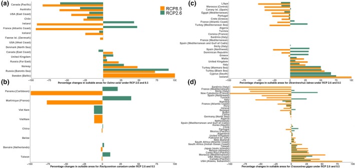
Percentage changes in potential suitable mariculture area for countries currently farming selected species by the middle of the century (average between 2040 and 2060) relative to 2000s (average between 1995 and 2015) under RCP 2.6 and 8.5. (a) Atlantic salmon, (b) Cobia, (c) European bass, (d) Pacific cupped oyster
4. DISCUSSION
In recent years, the growth of global mariculture production has helped maintain a relatively stable seafood supply in the world (Campbell & Pauly, 2013; FAO, 2018), with aquaculture being considered the fastest growing food system globally (FAO, 2018). However, our findings highlight the uncertainties associated with the future development of global mariculture (both marine and brackish aquaculture). We projected a large‐scale redistribution of mariculture species diversity and changes in potential areas suitable for mariculture in the world's oceans. Specifically, under climate change, we projected gains in MSRP at higher latitudes, and losses throughout much of the tropics, in line with previous findings (Froehlich et al., 2018; Handisyde et al., 2006; Porter et al., 2014).
Species diversification has been identified as an essential strategy toward increasing food supply from aquaculture: a necessary action to improve the aquaculture food sector's profitability and flexibility (Harvey et al., 2016). Some studies (Harvey et al., 2016; Le François, Jobling, & Carter, 2010) have argued that species diversification could lend the sector resilience, particularly under climate change. Our results clearly highlight that such species diversification would need to consider the projected impacts of a changing climate on the diversity of species that can be potentially farmed, particularly in the tropics that currently boast high species richness, but stand to register the greatest losses in the future. Such care is all the more needed, given the sector's contribution to nutrition and food security (Thilsted et al., 2016), and considering projected declines in capture fisheries under climate change (Cheung et al., 2010). Also, suitable marine areas for valuable economic species such as Atlantic salmon, Cobia and European bass will be lost, particularly in top producing countries. However, careful selection of species could avoid some of the socio‐economic losses linked to climate change. For instance, while Atlantic salmon farming marine areas along Canada's Pacific coast EEZ are projected to be impacted under both greenhouse gases scenarios (i.e. RCP 2.6 and 8.5), the potentially suitable marine area for Pacific cupped oyster stands to increase substantially in this EEZ.
Although our study projected that future Arctic ocean conditions would be suitable for mariculture operations, and could see an increase in MSRP, this region is unlikely to support mariculture development from a conservation and governance perspective. While mariculture operations in the Arctic region contributed about 2% of total world aquaculture production in 2015 (Troell, Eide, Isaksen, Hermansen, & Crepin, 2017), Arctic ocean ecosystems are generally considered sensitive to human activities (Meier et al., 2014; Riedel, 2014). Thus, the expansion of mariculture activities in the Arctic could conceivably have a considerable impact on marine biodiversity and ecosystem functions. Such impacts would be exacerbated if the development of operations was to take place in the absence of effective environmental management and regulations, resulting in ecological impacts through, for example, excessive nutrient and chemical outflows from the farms (Ivanov, Smagina, Chivilev, & Kruglikov, 2013), escapes of farmed fish (Jensen et al., 2013), as well as the risk of disease and parasite transfer from farmed to wild stocks (Palm, 2011). Opening the Arctic region to aquaculture activities may also further exacerbate the region's vulnerability to climate change.
The important losses in marine diversity and potentially suitable area for mariculture projected under RCP 2.6 and RCP 8.5 for tropical regions underscore the considerable threat that climate change presents to areas that currently contribute a substantial amount to food fish production and that also depend on a large proportion of that production for local food security, income and employment (FAO, 2018). Aquaculture is viewed as critical to supporting food security throughout developing tropical countries due to the static or declining contributions by capture fisheries to the food fish basket (Brummett, Lazard, & Moehl, 2008). However, mariculture may not be the panacea to nutritional security, particularly for developing countries, has it is perceived (Bogard, Marks, Mamun, & Thilsted, 2017; Golden et al., 2016).
Our findings underline the importance of this uncertainty. Our results show climate change impacts on mollusc mariculture to be more apparent than finfish. This might be because of the northward shift in potentially suitable marine areas for finfish and the resilience of finfish (Froehlich et al., 2018) under global increasing greenhouse gases. While our study focused on species richness in mariculture, our results are in line with those of other studies that have examined the role of climate change on aquaculture (Froehlich et al., 2018; Klinger et al., 2017). Notably, the three studies point to a loss in suitable marine area and biomass in mariculture production in the tropics and subtropical region, and conversely an increase in both suitable area and biomass in temperate regions under increasing greenhouse gas emissions. In addition, for countries where mariculture has been an essential part of the coastal economy (Froehlich et al., 2018; e.g. China), if the loss in potentially suitable mariculture area were to translate into a reduction in growth performance and subsequent reduction in aquaculture production output, this could be detrimental to the sustainable development of these coastal communities (Singh et al., 2018).
Our results further lend credence to previous findings pointing out that changes in ocean conditions because of climate change would affect the suitable environmental area that supports the farming of aquatic species in open water farming systems (Froehlich et al., 2018; Klinger et al., 2017; Oyinlola et al., 2018). Mariculture species perform best within a stress‐free environment. Hence, to optimize production and be most cost‐effective, farmers strive to locate ocean‐based facilities within the optimal oceanic environment for the farmed species (Benetti, Benetti, Rivera, Sardenberg, & O’Hanlon, 2010). In this study, we ascertained the best combination of oceanic parameters to achieve optimal growth conditions for each of the 85 currently most commonly farmed species (Basille et al., 2008; Oyinlola et al., 2018) using three different models. Such quantitative methods and models represent useful tools to inform the aquaculture sector of the possible risks and likely vulnerabilities of their current and planned operations under climate change. However, other socio‐economic and governance factors play essential roles in determining overall mariculture productivity (Davies et al., 2019), and future work would benefit from building on work presented in this study to focus on an evaluation of these dimensions for the future of mariculture under climate change.
While this study focused specifically on the effects of climate change on the environmental suitability for mariculture species, there are a number of other direct and indirect impacts of climate change on mariculture that may render the future viability and sustainability of mariculture production uncertain. Body size of finfish is expected to decline for open water systems due to increases in temperature limiting oxygen for optimal growth (Pauly & Cheung, 2017). Higher temperatures could also exacerbate the prevalence of aquaculture‐related diseases and parasitic infections (Karvonen, Rintamaki, Jokela, & Valtonen, 2010; Lafferty et al., 2015; Walker & Mohan, 2009) resulting in sizeable economic losses to producing countries, in addition to estimated losses in potentially suitable mariculture areas. Harmful algal blooms (HABs) have caused major mortality losses in the aquaculture sector in different regions of the world (e.g. pacific Canada and Chile; Apablaza et al., 2017; Haigh & Esenkulova, 2014; Lembeye, 2008; Rensel & Whyte, 2003; Rosa et al., 2013), leading to substantial losses in revenue and employment (Rensel & Whyte, 2003). Studies have shown that under increasing greenhouse gas emissions, the frequency, intensity and geographic extent of HABs may also increase (Berdalet et al., 2015; Glibert et al., 2014). Simulations indicate that climate change will negatively impact the abundance and maximum catch potential of forage fish from capture fisheries (Cheung et al., 2016, 2010) leading to a possible reduction in fishmeal and fish oil supply, which may affect aquafeed production. Substantial declines in agricultural yields have been projected to occur in most regions of the world (Nelson et al., 2009; Piao et al., 2010; Schlenker & Lobell, 2010), further impacting the supply of (plant source in) aquafeeds. Future growth and production estimates also will be shaped by a number of indirect socio‐economic factors such as population, technology and consumption patterns. Future studies should focus on how these may impact mariculture production in the future.
Our approach of integrating three models to simulate changes in the potentially suitable marine area available for farming and MSRP enables us to explore the structural uncertainty of projected species distributions based on their environment (Cheung et al., 2016). GBM and MAXENT had the highest AUC values. In the case of GBM, this may be due to the model's ability to build some regression trees sequentially from pseudo‐residuals by least squares at each iteration (Friedman, 2002). This attribute helps GBM correct errors made by previously trained regression trees. In GBM, a ‘tree’ is made up of random subsamples of the data set incrementally improving the model (Moisen et al., 2006). With MAXENT, the model provides the user with the ability to weight input variables (Jones & Cheung, 2014), thereby preventing over‐fitting of the model by determining how much the likelihood should be penalized. Likelihood penalization is necessary to control model complexity and the variance of the estimated suitability index (Hutchinson et al., 2015; Murphy, 2012).
Nevertheless, there are limitations to our modelling approach. SDMs may not always adequately quantify species' environmental preference ranges. This is because SDMs assume that environmental preference ranges are determined only by climate variables and that an equilibrium exists between the realized species range and its potential range as defined by climate variables (Pearson & Dawson, 2003). Also, model inaccuracies may occur particularly in coastal waters because of the resolution of the farm location data set and how we allocated mariculture farm locations so they match the resolution of the climate data (e.g. based on 0.5° latitude × 0.5° longitude). The ESMs projections are available at 50 km resolution, while farm locations were mapped at a resolution of 1 km. Hence, ESM data miss local‐level variability typically experienced at the farm level. Other studies (Barbosa, Real, & Vargas, 2010; Ehrlen & Morris, 2015; Freer, Partridge, Tarling, Collins, & Genner, 2018; Guisan & Thuiller, 2005) have arrived at similar conclusions regarding the limitations and uncertainty in the use of ESM projections in combination with species occurrence data. The aim of this study was to focus on the future of aquaculture at the global level and examine regional changes in potential mariculture species richness (see Supplementary Information for averaged results across EEZs). Future studies should focus on projections at the regional and national scale and use downscaled climate data and other relevant data sets at resolutions relevant to such analyses.
Our results underscore that future climate change impacts will impact some regions more strongly than others, and can help inform actions required to mitigate and adapt to the effects of climate change on the future suitability of ocean sites for farming aquatic organisms for food production. While our findings clearly highlight that future changes in the marine environment will significantly impact mariculture activities, extreme events and their likelihood to increase in severity and frequency will also need to be given due consideration. Similarly, proximity to markets, conflicts with other oceans users and availability of local aquafeed ingredients will continue to be important determinants of aquaculture species diversification and production. Integration of these considerations together with a review of marine aquaculture zoning and site selection factoring in climate change will be needed to improve the adaptive capacity of the sector, contribute to reducing uncertainties and minimize impacts on production and dependent socio‐economics of mariculture countries. In addition, hybridization and development of new species strains that have better survival rates at higher temperatures and lower oxygen levels should be encouraged through research and development. Future increases and improvements in cost‐effective technology should also improve land‐based operations. Lastly, it is important to consider that the sustainability of the future expansion of mariculture may in part, be linked to the effectiveness of conservation and governance measures. Policymakers must set clear objectives for future mariculture sustainability efforts and ensure the rule of law and due process are followed and enforced.
AUTHOR CONTRIBUTIONS
Muhammed A. Oyinlola and William W. L. Cheung conceptualized the study. Muhammed A. Oyinlola and Gabriel Reygondeau contributed towards data curation, resources and software. Muhammed A. Oyinlola involved in formal analysis, investigation, project administration, visualization and writing and drafting of the study. William W. L. Cheung involved in funding acquisition. Muhammed A. Oyinlola, Gabriel Reygondeau and William W. L. Cheung involved in methodology. Gabriel Reygondeau and William W. L. Cheung supervised the project. Muhammed A. Oyinlola, Gabriel Reygondeau, Colette C. C. Wabnitz and William W.L. Cheung validated the study. Muhammed A. Oyinlola, Gabriel Reygondeau, Colette C. C. Wabnitz and William W. L. Cheung involved in writing and review and editing.
Supporting information
ACKNOWLEDGEMENT
This study is a contribution by the Nippon Foundation‐the University of British Columbia Nereus Program, an interdisciplinary ocean research program. W. Cheung also acknowledges funding support from the Natural Sciences and Engineering Research Council of Canada. The authors do not have any conflicts of interest to declare.
Oyinlola MA, Reygondeau G, Wabnitz CCC, Cheung WWL. Projecting global mariculture diversity under climate change. Glob Change Biol. 2020;26:2134–2148. 10.1111/gcb.14974
DATA AVAILABILITY STATEMENT
Mariculture locations and production data are available from the Sea Around Us global mariculture database (http://www.seaaroundus.org/). Species ecological information from FishBase (http://www.fishbase.org/) and the Encyclopaedia of life (http://eol.org/). Species occurrence data from Ocean Biogeographic Information System (OBIS, http://www.iobis.org/), Global Biodiversity Information Facility (GBIF, http://www.gbif.org/), FishBase (http://www.fishbase.org/) and the International Union for the Conservation of Nature (IUCN, http://www.iucnredlist.org/technical-documents/spatial-data). Annual climatology for the period 1955–2012 for temperature, salinity, dissolved oxygen concentration and silicate concentration were obtained from the World Ocean Atlas 2013 (http://www.nodc.noaa.gov/OC5/woa13/). Euphotic depth and chlorophyll‐a concentration annual climatology for the period from 1998 to 2012 were downloaded from the Ocean Colour website (http://oceancolor.gsfc.nasa.gov). Ocean current velocity data (1992–2002) from the ECCO Project (http://www.ecco-group.org). Environmental parameters: sea surface temperature, dissolved oxygen concentration, chlorophyll‐a concentration, salinity, pH, silicate concentration and euphotic depth are from the three ESMs that were part of the Coupled Models Inter‐comparison Project Phase 5 (CMIP5): (a) the Geophysical Fluid Dynamics Laboratory Earth System Model 2M (GFDLESM2M), (b) the Institute Pierre Simon Laplace coupled model version 5 (IPSL; IPSL‐CM5‐MR), and (c) the Max Planck Institute for Meteorology Earth System Model (MPI‐ESM‐MR).
REFERENCES
- Alexandratos, N. , & Bruinsma, J. (2012). World agriculture towards 2030/2050: The 2012 revision (p. 4). ESA Working paper No. 12‐03. Rome, Italy: FAO. [Google Scholar]
- Apablaza, P. , Frisch, K. , Brevik, O. J. , Smage, S. B. , Vallestad, C. , Duesund, H. , … Nylund, A. (2017). Primary isolation and characterization of Tenacibaculum maritimum from Chilean Atlantic salmon mortalities associated with a Pseudochattonella spp. algal bloom. The Journal of Aquatic Animal Health, 29(3), 143–149. 10.1080/08997659.2017.1339643 [DOI] [PubMed] [Google Scholar]
- Ayyadevara, V. K. (2018). Gradient boosting machine In Pro machine learning algorithms: A hands‐on approach to implementing algorithms in python and R (pp. 117–134). Berkeley, CA: Apress. [Google Scholar]
- Barange, M. , Bahri, T. , Beveridge, M. C. M. , Cochrane, K. L. , Funge‐Smith, S. , & Poulain, F. (Eds.). (2018). Impacts of climate change on fisheries and aquaculture: Synthesis of current knowledge, adaptation and mitigation options (628: pp.). FAO Fisheries and Aquaculture Technical Paper No. 627. Rome, Italy: FAO. [Google Scholar]
- Barange, M. , & Perry, R. I. (2009). Physical and ecological impacts of climate change relevant to marine and inland capture fisheries and aquaculture. Climate change implications for fisheries and aquaculture.
- Barbosa, A. M. , Real, R. , & Vargas, J. M. (2010). Use of coarse‐resolution models of species' distributions to guide local conservation inferences. Conservation Biology, 24(5), 1378–1387. 10.1111/j.1523-1739.2010.01517.x [DOI] [PubMed] [Google Scholar]
- Basille, M. , Calenge, C. , Marboutin, É. , Andersen, R. , & Gaillard, J.‐M. (2008). Assessing habitat selection using multivariate statistics: Some refinements of the ecological‐niche factor analysis. Ecological Modelling, 211(1–2), 233–240. 10.1016/j.ecolmodel.2007.09.006 [DOI] [Google Scholar]
- Baulcombe, D. , Crute, I. , Davies, B. , Dunwell, J. , Gale, M. , Jones, J. … Toulmin, C. (2009). Reaping the benefits: Science and the sustainable intensification of global agriculture. London, UK: The Royal Society. [Google Scholar]
- Benetti, D. D. , Benetti, G. I. , Rivera, J. A. , Sardenberg, B. , & O’Hanlon, B. (2010). Site selection criteria for open ocean aquaculture. Marine Technology Society Journal, 44(3), 22–35. 10.4031/MTSJ.44.3.11 [DOI] [Google Scholar]
- Berdalet, E. , Fleming, L. E. , Gowen, R. , Davidson, K. , Hess, P. , Backer, L. C. , … Enevoldsen, H. (2015). Marine harmful algal blooms, human health and wellbeing: Challenges and opportunities in the 21st century. Journal of the Marine Biological Association of the United Kingdom, 96(1), 61–91. 10.1017/S0025315415001733 [DOI] [PMC free article] [PubMed] [Google Scholar]
- Bogard, J. R. , Marks, G. C. , Mamun, A. , & Thilsted, S. H. (2017). Non‐farmed fish contribute to greater micronutrient intakes than farmed fish: Results from an intra‐household survey in rural Bangladesh. Public Health Nutrition, 20(4), 702–711. 10.1017/S1368980016002615 [DOI] [PMC free article] [PubMed] [Google Scholar]
- Bogard, J. R. , Thilsted, S. H. , Marks, G. C. , Wahab, M. A. , Hossain, M. A. R. , Jakobsen, J. , & Stangoulis, J. (2015). Nutrient composition of important fish species in Bangladesh and potential contribution to recommended nutrient intakes. Journal of Food Composition and Analysis, 42, 120–133. 10.1016/j.jfca.2015.03.002 [DOI] [Google Scholar]
- Brummett, R. E. , Lazard, J. , & Moehl, J. (2008). African aquaculture: Realizing the potential. Food Policy, 33(5), 371–385. 10.1016/j.foodpol.2008.01.005 [DOI] [Google Scholar]
- Busby, J. (1991). BIOCLIM‐a bioclimate analysis and prediction system. Plant Protection Quarterly, 61, 8–9. [Google Scholar]
- Campbell, B. , & Pauly, D. (2013). Mariculture: A global analysis of production trends since 1950. Marine Policy, 39, 94–100. 10.1016/j.marpol.2012.10.009 [DOI] [Google Scholar]
- Cheung, W. W. L. , Brodeur, R. D. , Okey, T. A. , & Pauly, D. (2015). Projecting future changes in distributions of pelagic fish species of Northeast Pacific shelf seas. Progress in Oceanography, 130, 19–31. 10.1016/j.pocean.2014.09.003 [DOI] [Google Scholar]
- Cheung, W. W. L. , Jones, M. C. , Reygondeau, G. , Stock, C. A. , Lam, V. W. Y. , & Frölicher, T. L. (2016). Structural uncertainty in projecting global fisheries catches under climate change. Ecological Modelling, 325, 57–66. 10.1016/j.ecolmodel.2015.12.018 [DOI] [Google Scholar]
- Cheung, W. W. L. , Lam, V. W. Y. , Sarmiento, J. L. , Kearney, K. , Watson, R. , & Pauly, D. (2009). Projecting global marine biodiversity impacts under climate change scenarios. Fish and Fisheries, 10(3), 235–251. 10.1111/j.1467-2979.2008.00315.x [DOI] [Google Scholar]
- Cheung, W. W. L. , Lam, V. W. Y. , Sarmiento, J. L. , Kearney, K. , Watson, R. E. G. , Zeller, D. , & Pauly, D. (2010). Large‐scale redistribution of maximum fisheries catch potential in the global ocean under climate change. Global Change Biology, 16(1), 24–35. 10.1111/j.1365-2486.2009.01995.x [DOI] [Google Scholar]
- Cochrane, K. , De Young, C. , Soto, D. , & Bahri, T. (2009). Climate change implications for fisheries and aquaculture. FAO. Fisheries and Aquaculture Technical Paper,530(212). [Google Scholar]
- Davies, I. P. , Carranza, V. , Froehlich, H. E. , Gentry, R. R. , Kareiva, P. , & Halpern, B. S. (2019). Governance of marine aquaculture: Pitfalls, potential, and pathways forward. Marine Policy, 104, 29–36. 10.1016/j.marpol.2019.02.054 [DOI] [Google Scholar]
- De Silva, S. S. , & Soto, D. (2009). Climate change and aquaculture: Potential impacts, adaptation and mitigation. Climate change implications for fisheries and aquaculture: Overview of current scientific knowledge. FAO Fisheries and Aquaculture Technical Paper, 530, 151–212. [Google Scholar]
- Ehrlen, J. , & Morris, W. F. (2015). Predicting changes in the distribution and abundance of species under environmental change. Ecology Letters, 18(3), 303–314. 10.1111/ele.12410 [DOI] [PMC free article] [PubMed] [Google Scholar]
- Elith, J. , H. Graham, C. , P. Anderson, R. , Dudík, M. , Ferrier, S. , Guisan, A. , … E. Zimmermann, N. (2006). Novel methods improve prediction of species’ distributions from occurrence data. Ecography, 29, 129–151. 10.1111/j.2006.0906-7590.04596.x [DOI] [Google Scholar]
- Elith, J. , & Leathwick, J. R. (2009). Species distribution models: Ecological explanation and prediction across space and time. Annual Review of Ecology, Evolution, and Systematics, 40(1), 677–697. 10.1146/annurev.ecolsys.110308.120159 [DOI] [Google Scholar]
- FAO . (2004). Coordinating working party on fishery statistics. Handbook of fishery statistical standards (Vol. 260). Rome, Italy: FAO. [Google Scholar]
- FAO . (2014). The state of world fisheries and aquaculture. Opportunities and challenges. Rome, Italy: Food & Agriculture Org. [Google Scholar]
- FAO . (2018). The state of world fisheries and aquaculture 2018 – Meeting the sustainable development goals. Rome, Italy: FAO. [Google Scholar]
- Freer, J. J. , Partridge, J. C. , Tarling, G. A. , Collins, M. A. , & Genner, M. J. (2018). Predicting ecological responses in a changing ocean: The effects of future climate uncertainty. Marine Biology, 165(1), 7 10.1007/s00227-017-3239-1 [DOI] [PMC free article] [PubMed] [Google Scholar]
- Friedman, J. H. (2002). Stochastic gradient boosting. Computational Statistics & Data Analysis, 38(4), 367–378. 10.1016/S0167-9473(01)00065-2 [DOI] [Google Scholar]
- Froehlich, H. E. , Gentry, R. R. , & Halpern, B. S. (2018). Global change in marine aquaculture production potential under climate change. Nature Ecology & Evolution, 2(11), 1745–1750. 10.1038/s41559-018-0669-1 [DOI] [PubMed] [Google Scholar]
- Gattuso, J. P. , Magnan, A. , Bille, R. , Cheung, W. W. , Howes, E. L. , Joos, F. , … Turley, C. (2015). Contrasting futures for ocean and society from different anthropogenic CO(2) emissions scenarios. Science, 349(6243), aac4722 10.1126/science.aac4722 [DOI] [PubMed] [Google Scholar]
- Gentry, R. R. , Froehlich, H. E. , Grimm, D. , Kareiva, P. , Parke, M. , Rust, M. , … Halpern, B. S. (2017). Mapping the global potential for marine aquaculture. Nature Ecology & Evolution, 1(9), 1317–1324. 10.1038/s41559-017-0257-9 [DOI] [PubMed] [Google Scholar]
- Giles, G. E. , Mahoney, C. R. , & Kanarek, R. B. (2019). Omega‐3 fatty acids and cognitive behavior. 313–355. 10.1016/b978-0-12-815238-6.00020-1 [DOI]
- Glibert, P. M. , Icarus Allen, J. , Artioli, Y. , Beusen, A. , Bouwman, L. , Harle, J. , … Holt, J. (2014). Vulnerability of coastal ecosystems to changes in harmful algal bloom distribution in response to climate change: Projections based on model analysis. Global Change Biology, 20(12), 3845–3858. 10.1111/gcb.12662 [DOI] [PubMed] [Google Scholar]
- Golden, C. , Allison, E. H. , Cheung, W. W. L. , Dey, M. M. , Halpern, B. S. , McCauley, D. J. , … Myers, S. S. (2016). Fall in fish catch threatens human health. Natural, 534(7607), 317–320. [DOI] [PubMed] [Google Scholar]
- Guisan, A. , & Thuiller, W. (2005). Predicting species distribution: Offering more than simple habitat models. Ecology Letters, 8(9), 993–1009. 10.1111/j.1461-0248.2005.00792.x [DOI] [PubMed] [Google Scholar]
- Guisan, A. , & Zimmermann, N. E. (2000). Predictive habitat distribution models in ecology. Ecological Modelling, 135(2), 147–186. [Google Scholar]
- Haigh, N. , & Esenkulova, S. (2014). Economic losses to the British Columbia salmon aquaculture industry due to harmful algal blooms, 2009–2012. PICES Scientific Report, 47, 2. [Google Scholar]
- Hall, S. J. , Delaporte, A. , Phillips, M. J. , Beveridge, M. , & O′Keefe, M. (2011). Blue frontiers: Managing the environmental cost of aquaculture, 92. Penang: The WorldFish Center. [Google Scholar]
- Handisyde, N. T. , Ross, L. G. , Badjeck, M. C. , & Allison, E. H. (2006). The effects of climate change on world aquaculture: A global perspective. Aquaculture and Fish Genetics Research Programme, Stirling Institute of Aquaculture. Final Technical Report, DFID, Stirling, 151.
- Harley, C. D. G. , Randall Hughes, A. , Hultgren, K. M. , Miner, B. G. , Sorte, C. J. B. , Thornber, C. S. , … Williams, S. L. (2006). The impacts of climate change in coastal marine systems. Ecology Letters, 9(2), 228–241. 10.1111/j.1461-0248.2005.00871.x [DOI] [PubMed] [Google Scholar]
- Harris, W. S. , Miller, M. , Tighe, A. P. , Davidson, M. H. , & Schaefer, E. J. (2008). Omega‐3 fatty acids and coronary heart disease risk: Clinical and mechanistic perspectives. Atherosclerosis, 197(1), 12–24. 10.1016/j.atherosclerosis.2007.11.008 [DOI] [PubMed] [Google Scholar]
- Harvey, B. , Soto, D. , Carolsfeld, J. , Beveridge, M. , & Bartley, D. M. (2016). Planning for aquaculture diversification: The importance of climate change and other drivers. In FAO Technical Workshop, 23–25.
- Hijmans, R. J. , Phillips, S. , Leathwick, J. , Elith, J. , & Hijmans, M. R. J. (2017). Package ‘dismo’. Circles, 9(1), 1–68. [Google Scholar]
- Hilborn, R. , Banobi, J. , Hall, S. J. , Pucylowski, T. , & Walsworth, T. E. (2018). The environmental cost of animal source foods. Frontiers in Ecology and the Environment, 16(6), 329–335. 10.1002/fee.1822 [DOI] [Google Scholar]
- HLPE . (2014). Sustainable fisheries and aquaculture for food security and nutrition. A report by the High Level Panel of Experts on Food Security and Nutrition of the Committee on World Food Security, Rome 2014.
- Hutchinson, G. E. (1959). Homage to Santa Rosalia or why are there so many kinds of animals? The American Naturalist, 93(870), 145–159. 10.1086/282070 [DOI] [Google Scholar]
- Hutchinson, R. A. , Valente, J. J. , Emerson, S. C. , Betts, M. G. , Dietterich, T. G. , & Freckleton, R. (2015). Penalized likelihood methods improve parameter estimates in occupancy models. Methods in Ecology and Evolution, 6(8), 949–959. 10.1111/2041-210x.12368 [DOI] [Google Scholar]
- Innis, S. M. (2008). Dietary omega 3 fatty acids and the developing brain. Brain Research, 1237, 35–43. 10.1016/j.brainres.2008.08.078 [DOI] [PubMed] [Google Scholar]
- Ivanov, M. V. , Smagina, D. S. , Chivilev, S. M. , & Kruglikov, O. E. (2013). Degradation and recovery of an Arctic benthic community under organic enrichment. Hydrobiologia, 706(1), 191–204. 10.1007/s10750-012-1298-3 [DOI] [Google Scholar]
- Jensen, A. J. , Karlsson, S. , Fiske, P. , Hansen, L. P. , Hindar, K. , & Østborg, G. M. (2013). Escaped farmed Atlantic salmon grow, migrate and disperse throughout the Arctic Ocean like wild salmon. Aquaculture Environment Interactions, 3(3), 223–229. 10.3354/aei00064 [DOI] [Google Scholar]
- Jones, M. C. , & Cheung, W. W. L. (2014). Multi‐model ensemble projections of climate change effects on global marine biodiversity. ICES Journal of Marine Science, 72(3), 741–752. 10.1093/icesjms/fsu172 [DOI] [Google Scholar]
- Kapetsky, J. M. , Aguilar‐Manjarrez, J. , & Jenness, J. (2013). A global assessment of offshore mariculture potential from a spatial perspective. FAO Fisheries and Aquaculture Technical Paper, 549.
- Karvonen, A. , Rintamaki, P. , Jokela, J. , & Valtonen, E. T. (2010). Increasing water temperature and disease risks in aquatic systems: Climate change increases the risk of some, but not all, diseases. International Journal for Parasitology, 40(13), 1483–1488. 10.1016/j.ijpara.2010.04.015 [DOI] [PubMed] [Google Scholar]
- Klinger, D. H. , Levin, S. A. , & Watson, J. R. (2017). The growth of finfish in global open‐ocean aquaculture under climate change. Proceedings of the Royal Society B: Biological Sciences, 284(1864), 10.1098/rspb.2017.0834 [DOI] [PMC free article] [PubMed] [Google Scholar]
- Lafferty, K. D. , Harvell, C. D. , Conrad, J. M. , Friedman, C. S. , Kent, M. L. , Kuris, A. M. , … Saksida, S. M. (2015). Infectious diseases affect marine fisheries and aquaculture economics. Annual Review of Marine Science, 7, 471–496. 10.1146/annurev-marine-010814-015646 [DOI] [PubMed] [Google Scholar]
- Larsen, R. , Eilertsen, K. E. , & Elvevoll, E. O. (2011). Health benefits of marine foods and ingredients. Biotechnology Advances, 29(5), 508–518. 10.1016/j.biotechadv.2011.05.017 [DOI] [PubMed] [Google Scholar]
- Le François, N. R. , Jobling, M. , & Carter, C. (2010). Finfish aquaculture diversification. Oxfordshire, UK: Cabi. [Google Scholar]
- Legendre, P. , & Legendre, L. F. (2012). Numerical ecology (Vol. 24). Amsterdam, The Netherlands: Elsevier. [Google Scholar]
- Lembeye, G. (2008). Harmful algal blooms in the austral Chilean channels and fjords In Silva N. & Palma S. (Eds.), Progress in the oceanographic knowledge of Chilean interior waters, from Puerto Montt to Cape Horn (pp. 99–103). Valparaíso, Chile: Comité Oceanográfico Nacional ‐ Pontificia Universidad Católica de Valparaíso. [Google Scholar]
- MATLAB and Statistics Toolbox Release 2018b . (2018). The MathWorks, Inc., Natick, MA.
- Meier, W. N. , Hovelsrud, G. K. , van Oort, B. E. H. , Key, J. R. , Kovacs, K. M. , Michel, C. , … Reist, J. D. (2014). Arctic sea ice in transformation: A review of recent observed changes and impacts on biology and human activity. Reviews of Geophysics, 52(3), 185–217. 10.1002/2013RG000431 [DOI] [Google Scholar]
- Meyer, B. J. , Mann, N. J. , Lewis, J. L. , Milligan, G. C. , Sinclair, A. J. , & Howe, P. R. (2003). Dietary intakes and food sources of omega‐6 and omega‐3 polyunsaturated fatty acids. Lipids, 38(4), 391–398. 10.1007/s11745-003-1074-0 [DOI] [PubMed] [Google Scholar]
- Moisen, G. G. , Freeman, E. A. , Blackard, J. A. , Frescino, T. S. , Zimmermann, N. E. , & Edwards, T. C. Jr (2006). Predicting tree species presence and basal area in Utah: A comparison of stochastic gradient boosting, generalized additive models, and tree‐based methods. Ecological Modelling, 199(2), 176–187. 10.1016/j.ecolmodel.2006.05.021 [DOI] [Google Scholar]
- Murphy, K. P. (2012). Machine learning: A probabilistic perspective. Cambridge, MA: The MIT Press. [Google Scholar]
- Nelson, G. C. , Rosegrant, M. W. , Koo, J. , Robertson, R. , Sulser, T. , Zhu, T. , … David, L. (2009). Climate change: Impact on agriculture and costs of adaptation. Washington, DC: International Food Policy Research Institute. [Google Scholar]
- Newbold, T. (2018). Future effects of climate and land‐use change on terrestrial vertebrate community diversity under different scenarios. Proceedings of the Royal Society B: Biological Sciences, 285(1881), 10.1098/rspb.2018.0792 [DOI] [PMC free article] [PubMed] [Google Scholar]
- Newell, R. I. (2004). Ecosystem influences of natural and cultivated populations of suspension‐feeding bivalve molluscs: A review. Journal of Shellfish Research, 23(1), 51–62. [Google Scholar]
- Oyinlola, M. A. , Reygondeau, G. , Wabnitz, C. C. C. , Troell, M. , & Cheung, W. W. L. (2018). Global estimation of areas with suitable environmental conditions for mariculture species. PLoS ONE, 13(1), e0191086 10.1371/journal.pone.0191086 [DOI] [PMC free article] [PubMed] [Google Scholar]
- Palm, H. W. (2011). Fish parasites as biological indicators in a changing world: Can we monitor environmental impact and climate change? In Mehlhorn H. (Ed.), Progress in parasitology (pp. 223–250). Berlin, Heidelberg: Springer, Berlin Heidelberg. [Google Scholar]
- Pauly, D. , & Cheung, W. W. L. (2017). Sound physiological knowledge and principles in modeling shrinking of fishes under climate change. Global Change Biology, 24(1), e15–e26. 10.1111/gcb.13831 [DOI] [PubMed] [Google Scholar]
- Pearson, R. G. , & Dawson, T. P. (2003). Predicting the impacts of climate change on the distribution of species: Are bioclimate envelope models useful? Global Ecology and Biogeograph, 12(5), 361–371. 10.1046/j.1466-822X.2003.00042.x [DOI] [Google Scholar]
- Phillips, B. F. , & Pérez‐Ramírez, M. E. (2017). Climate change impacts on fisheries and aquaculture: A global analysis (Vol. 1). Hoboken, NJ: John Wiley & Sons. [Google Scholar]
- Phillips, S. J. , Anderson, R. P. , & Schapire, R. E. (2006). Maximum entropy modeling of species geographic distributions. Ecological Modelling, 190(3–4), 231–259. 10.1016/j.ecolmodel.2005.03.026 [DOI] [Google Scholar]
- Phillips, S. J. , Dudík, M. , Elith, J. , Graham, C. H. , Lehmann, A. , Leathwick, J. , & Ferrier, S. (2009). Sample selection bias and presence‐only distribution models: Implications for background and pseudo‐absence data. Ecological Applications, 19(1), 181–197. 10.1890/07-2153.1 [DOI] [PubMed] [Google Scholar]
- Piao, S. , Ciais, P. , Huang, Y. , Shen, Z. , Peng, S. , Li, J. , … Fang, J. (2010). The impacts of climate change on water resources and agriculture in China. Nature, 467(7311), 43–51. 10.1038/nature09364 [DOI] [PubMed] [Google Scholar]
- Pilditch, C. A. , Grant, J. , & Bryan, K. R. (2001). Seston supply to sea scallops (Placopecten magellanicus) in suspended culture. Canadian Journal of Fisheries and Aquatic Sciences, 58(2), 241–253. 10.1139/cjfas-58-2-241 [DOI] [Google Scholar]
- Polce, C. , Termansen, M. , Aguirre‐Gutiérrez, J. , Boatman, N. D. , Budge, G. E. , Crowe, A. , … Biesmeijer, J. C. (2013). Species distribution models for crop pollination: A modelling framework applied to Great Britain. PLoS ONE, 8(10), e76308 10.1371/journal.pone.0076308 [DOI] [PMC free article] [PubMed] [Google Scholar]
- Porter, J. R. , Xie, L. , Howden, M. , Iqbal, M. M. , Lobell, D. , Travasso, M. I. … Hakala, K. (2014). Food security and food production systems. Methods, 7, 1–1. [Google Scholar]
- R Core Team . (2018). R: A language and environment for statistical computing. Retrieved from https://www.r-project.org/ [Google Scholar]
- Rensel, J. E. , & Whyte, J. N. C. (2003). Finfish mariculture and harmful algal blooms. Manual on harmful marine microalgae. Monographs on Oceanographic Methodology, 11, 693–722. [Google Scholar]
- Riedel, A. (2014). The arctic marine environment In Tedsen E., Cavalieri S., & Kraemer R. A. (Eds.), Arctic marine governance: Opportunities for transatlantic cooperation (pp. 21–43). Berlin, Heidelberg: Springer, Berlin Heidelberg. [Google Scholar]
- Rosa, M. , Holohan, B. A. , Shumway, S. E. , Bullard, S. G. , Wikfors, G. H. , Morton, S. , & Getchis, T. (2013). Biofouling ascidians on aquaculture gear as potential vectors of harmful algal introductions. Harmful Algae, 23, 1–7. 10.1016/j.hal.2012.11.008 [DOI] [Google Scholar]
- Schlenker, W. , & Lobell, D. B. (2010). Robust negative impacts of climate change on African agriculture. Environmental Research Letters, 5(1), 014010 10.1088/1748-9326/5/1/014010 [DOI] [Google Scholar]
- Sing, T. , Sander, O. , Beerenwinkel, N. , & Lengauer, T. (2005). ROCR: Visualizing classifier performance in R. Bioinformatics, 21(20), 3940–3941. [DOI] [PubMed] [Google Scholar]
- Singh, G. G. , Cisneros‐Montemayor, A. M. , Swartz, W. , Cheung, W. , Guy, J. A. , Kenny, T.‐A. , … Ota, Y. (2018). A rapid assessment of co‐benefits and trade‐offs among Sustainable Development Goals. Marine Policy, 93, 223–231. 10.1016/j.marpol.2017.05.030 [DOI] [Google Scholar]
- Thilsted, S. H. , Thorne‐Lyman, A. , Webb, P. , Bogard, J. R. , Subasinghe, R. , Phillips, M. J. , & Allison, E. H. (2016). Sustaining healthy diets: The role of capture fisheries and aquaculture for improving nutrition in the post‐2015 era. Food Policy, 61, 126–131. 10.1016/j.foodpol.2016.02.005 [DOI] [Google Scholar]
- Tocher, D. R. (2015). Omega‐3 long‐chain polyunsaturated fatty acids and aquaculture in perspective. Aquaculture, 449, 94–107. 10.1016/j.aquaculture.2015.01.010 [DOI] [Google Scholar]
- Troell, M. , Eide, A. , Isaksen, J. , Hermansen, O. , & Crepin, A. S. (2017). Seafood from a changing Arctic. Ambio, 46(Suppl. 3), 368–386. 10.1007/s13280-017-0954-2 [DOI] [PMC free article] [PubMed] [Google Scholar]
- Trujillo, P. , Piroddi, C. , & Jacquet, J. (2012). Fish farms at sea: The ground truth from Google Earth. PLoS ONE, 7(2), e30546 10.1371/journal.pone.0030546 [DOI] [PMC free article] [PubMed] [Google Scholar]
- UN . (2019). World population prospects: The 2019 revision, key findings and advance tables. Population Division, United Nations, New York.
- Walker, P. J. , & Mohan, C. V. (2009). Viral disease emergence in shrimp aquaculture: Origins, impact and the effectiveness of health management strategies. Reviews in Aquaculture, 1(2), 125–154. 10.1111/j.1753-5131.2009.01007.x [DOI] [PMC free article] [PubMed] [Google Scholar]
Associated Data
This section collects any data citations, data availability statements, or supplementary materials included in this article.
Supplementary Materials
Data Availability Statement
Mariculture locations and production data are available from the Sea Around Us global mariculture database (http://www.seaaroundus.org/). Species ecological information from FishBase (http://www.fishbase.org/) and the Encyclopaedia of life (http://eol.org/). Species occurrence data from Ocean Biogeographic Information System (OBIS, http://www.iobis.org/), Global Biodiversity Information Facility (GBIF, http://www.gbif.org/), FishBase (http://www.fishbase.org/) and the International Union for the Conservation of Nature (IUCN, http://www.iucnredlist.org/technical-documents/spatial-data). Annual climatology for the period 1955–2012 for temperature, salinity, dissolved oxygen concentration and silicate concentration were obtained from the World Ocean Atlas 2013 (http://www.nodc.noaa.gov/OC5/woa13/). Euphotic depth and chlorophyll‐a concentration annual climatology for the period from 1998 to 2012 were downloaded from the Ocean Colour website (http://oceancolor.gsfc.nasa.gov). Ocean current velocity data (1992–2002) from the ECCO Project (http://www.ecco-group.org). Environmental parameters: sea surface temperature, dissolved oxygen concentration, chlorophyll‐a concentration, salinity, pH, silicate concentration and euphotic depth are from the three ESMs that were part of the Coupled Models Inter‐comparison Project Phase 5 (CMIP5): (a) the Geophysical Fluid Dynamics Laboratory Earth System Model 2M (GFDLESM2M), (b) the Institute Pierre Simon Laplace coupled model version 5 (IPSL; IPSL‐CM5‐MR), and (c) the Max Planck Institute for Meteorology Earth System Model (MPI‐ESM‐MR).