Attribute‐based classification of European hydrophytes and its relationship to habitat utilization

SUMMARY

• 1Here we classify selected European hydrophytes into ‘attribute groups’ based on the possession of homogenous sets of characteristics, and explore the correspondence between these attribute groups, or individual attributes, and habitat use.
• 2Non‐hierarchical clustering was used to assign 120 species to twenty groups based on a matrix of categorical scores for literature‐ and field‐derived information covering seventeen intrinsic morphological and life‐history traits. Subdivision of some of these traits produced a total of 58 attributes (i.e. modalities). The robustness of this classification was confirmed by a high rate of reclassification (92%) under multiple discriminant analysis (MDA). The phylogenetic contribution was explored using ordination methods with taxonomy at family level acting as a covariable.
• 3Our approach differed from earlier classifications based on growth or life form because we regarded growth form plasticity as a property of the species and its range of growing conditions, rather than of each individual population, and we considered additional (e.g. regenerative) traits. However, some conventional life form groups were preserved (i.e. utricularids, isoetids, hydrocharids and lemnids).
• 4Some parallels existed with established theory on terrestrial plant growth strategies, but we used strictly intrinsic attributes relevant specifically to hydrophytes and our groups could not be decomposed into three or four primary strategies. Only finer levels of partitioning appear to be of fundamental and applied ecological relevance in hydrophytes.
• 5A principal components analysis ordination based on 26 attributes related to physical habitat utilization separated species and their attribute groups along axes relating to: (a) flow, substratum grade and organic matter content, scour frequency, and sedimentation; and (b) depth, water level stability and biotic disturbance. A MDA applied to species ordination scores indicated only a modest overall correspondence between attribute groups and habitat use (54% correct reclassification). Poor reclassification was the result of intergroup overlap (indicating alternative sets of attributes for a given habitat) or high intragroup variance in habitat utilization (indicating commonality of attributes between different habitats). These results are interpreted in terms of trade‐offs between resistance and resilience traits, ‘functional plasticity’ in traits, phylogenetic dependence in some groups and methodological constraints. The predictive potential of hydrophyte groups and their limitations are discussed.
• 6Redundancy analysis revealed a highly significant correlation between traits and habitat use (P < 0.01). Our attribute matrix explained 72% of variation in physical habitat use with eight attributes (i.e. turions, anchored emergent leaves, high or low body flexibility, high root:shoot biomass ratio, free‐floating surface or free‐floating submerged growth form, and annual life history) explaining half of this variation.
• 7Most attributes were mapped in accordance with habitat template predictions, although tests were confounded by the underlying correlation between spatial and temporal heterogeneity. The main features were: (a) a trade‐off between resistance‐type traits (related to stream lining, flexibility and anchorage) in more spatially heterogenous riverine and littoral zone habitats, and resilience type traits (i.e. turions, very small body size and free‐floating growth forms) in spatially simple, rarely disturbed habitats, such as backwaters and canals; and (b) a shift from high investment competitive traits with a low reproductive output in deep stable habitats to classically ruderal and desiccation resistance traits in shallow fluctuating habitats.

Introduction

Over the last 20 years, the use of various biological traits to assemble species into coherent non‐taxonomic groups has provided a valuable alternative approach for studying the ecology of a wide range of vegetation types ( Friedel, Bastin & Griffin, 1988; Grime, Hodgson & Hunt, 1988; Leishman & Westoby, 1992; Boutin & Keddy, 1993; Golluscio & Sala, 1993; Murphy et al., 1994 ; Smith, Shugart & Woodward, 1997), although botanists have long been aware of the basic concept ( Du Rietz, 1931). Functional approaches of this type are appealing because they synthesize large complex data sets, which are readily accessible only to taxonomists and habitat specialists, into smaller, more general and easily interpreted sets of attributes, including traits of known or potential adaptive value ( Keddy, 1989; Korner, 1993). For the assessment of ecosystem functioning, groups based on functional attributes also provide a more appropriate unit of currency than species richness ( MacGillivray et al., 1995 ; Grime, 1997). Having established functional group‐environment relationships, the impacts of perturbations can be predicted with broad sensitivity ( Shipley & Parent, 1991; Smith et al., 1993 ), rather than being dependent on the presence/absence of individual species which may merely reflect chance dispersal and recolonization events. The predictive value of functional groups has been appreciated for some time (e.g. Noble & Slatyer, 1980) and is of growing relevance to studies of the potential impacts of global climate change ( Woodward & Cramer, 1996; Diaz & Cabido, 1997).

In the case of aquatic macrophytes, the available non‐taxonomic classifications ( den Hartog & Segal, 1964; Hogeweg & Brenkert‐van Riert, 1969; Hutchinson, 1975) derive from the parallel concepts of growth form ( Du Rietz, 1931) and life form ( Raunkiaer, 1934), comprising groups of taxa which, although often unrelated, take morphologically comparable forms as an adaptation to a particular mode of life in a specific habitat ( Hutchinson, 1975). Their main application has been in the synecological approach to descriptions of water plant communities (e.g. den Hartog & Segal, 1964; Segal, 1968). Other than minor modifications by den Hartog & van der Velde (1988) and Wiegleb (1991), there have been few attempts to develop these basic classifications, yet it has been recognized for some time that defining assemblages of plants in terms of functional plant characteristics, rather than on taxono‐mic criteria ( Kautsky, 1988), could advance our understanding of macrophyte ecology. Hence, there have been several attempts to classify selected hydro‐phytes ( Grime et al., 1988 ; Kautsky, 1988; Rørslett, 1989; Murphy, Rørslett & Springuel, 1990; Spink, 1992) within the framework of groupings developed for terrestrial species ( Grime et al., 1988 ). The lack of fur‐ther progress may have several causes: (1) conventional classifications of hydrophytes are satisfactory (although comparison with a trait‐based classification using current data would be valid and worthwhile); (2) improvements are required, but effective sampling of hydrophytes and their habitats is perceived as too difficult; (3) trait data is too incomplete or fragmented to make a new classification possible; and (4) hydro‐phytes display such extreme phenotypic plasticity and wide ecological amplitude that classifications are pointless or have no predictive value.

In this paper, we use an inductive approach (sensu Woodward & Cramer,z 1996) to classify hydrophytes into groups of plants sharing the same attributes, where each attribute (i.e. modality sensu Chevenet et al., 1994 ) is the result of subdivision of a trait into simple categories (e.g. very large, large, medium or small, with appropriate size ranges, are attributes of the trait leaf size). We have resorted to the simple term ‘attribute groups’ since we share the reservations of Chapleau, Johansen & Williamson (1988) concerning the (ab)use of the term ‘strategy’. We have also resisted the rather vague term ‘functional group’ because the mechanistic relationship between traits and functions in hydrophytes is still poorly understood in many cases, and we have been unable to define specific functions. However, the traits which we use are of potential functional significance (sensu Lincoln et al., 1982) , and our groups could be re‐garded as functionally distinct in that each reflects a different emphasis on key plant processes such as resource acquisition, growth, reproduction and dispersal/colonization ( Botkin, 1975). Keddy (1992) has recommended that, rather than defining the functions (and traits which might best measure these functions) at the outset, a pragmatic approach is to measure a large number of traits on a large number of species and see what patterns emerge. Our species × traits matrix is the product of exhaustive literature searches and extensive fieldwork in European freshwater habitats which we believe offers a pragmatic alternative to large‐scale experimental screening.

We then examine the relationship between attribute groups, species attributes and habitat utilization. Grace (1993) has described ‘a partial correlation between the syndrome of functional attributes and the habitat relations’ in a study of clonal propagation methods in aquatic angiosperms, while expressing the need to consider entire growth form and life history in order to improve the predictiveness of this relationship. We believe that focusing jointly on individual attributes and plant attribute groups is preferable to considering traits in isolation since real species represent alternative combinations of attributes. We use a matrix of scores for physical habitat variables (subdivided as above into habitat characteristics) based on the known overall range of occurrence of individual aquatic macrophytes within north‐western Europe rather than focusing on a particular site or type of aquatic habitat. An advantage at this scale is that the direct match between species and environment is less likely to be obscured by the history of the local environment and the chance dispersal of organisms ( Townsend & Hildrew, 1994). If the environment is viewed as a nest of sieves through which species are sorted according to the traits they display before they can occupy a particular habitat, then two questions can be posed depending on the chosen perspective: (1) How much variation in the expression of a trait at the species or assemblage level can be explained by measurements of environmental variables? (Is mesh size a good predictor of particle diameter?); and (2) To what extent is current habitat utilization the product of existing traits? (Can particle diameter be used as an indicator of mesh size?) Here, because we are dealing with habitat utilization, i.e. the partial product of trait filtering, rather than extrinsic measurements of the environment, only the second question is pertinent.

We use the habitat template concept of Southwood ((1977), (1988)) as a context for this study. This concept has received significant support in a number of recent freshwater ecological studies (e.g. Statzner, Resh & Doledec, 1994; Statzner et al., 1997 ; Townsend, Doledec & Scarsbrook, 1997), and has also formed the framework for studies of brackish water macrophytes ( Kautsky, 1988), riverine Potamogeton species ( Wiegleb, Brux & Herr, 1991), riverine bryophytes ( Muotka & Virtanen, 1995), marine algae ( Steneck & Dethier, 1994) and stream periphyton ( Biggs, Stevenson & Lowe, 1998). Stearns (1976), Southwood ((1977), (1988)), Grime ((1977), (1979)) and Grime et al. (1997) have offered general predictions about the combinations of traits likely to evolve in habitats of contrasting spatial and temporal variability, and there have been numerous, direct or indirect tests of these predictions for terrestrial and wetland vegetation (e.g. Day et al., 1988 ; Gaudet & Keddy, 1988; Shipley & Keddy, 1988; Shipley et al., 1989 ; Moore & Noble, 1990; Montalvo et al., 1991 ; Fernandez Ales, Laffarga & Ortega, 1993; Smith, Mark & Wilson, 1995; Chapin et al., 1996 ; Prach, Pysek & Šmilauer, 1997).

In the case of hydrophytes, Grace (1993) offered predictions on the relationship between the functional attributes of different methods of clonal propagation and habitat conditions, such as disturbance rate, resource availability, spatial heterogeneity and exposure to mechanical stress. Townsend & Hildrew (1994) have listed general traits expected to occur in aquatic organisms in different regions of a habitat templet for riverine environments; their predictions were extensively tested in a multidisciplinary study of the Upper Rhône, France, ( Statzner et al., 1994 ) for a range of taxa, including aquatic macrophytes ( Bornette et al., 1994 ), and have been tested subsequently elsewhere using macroinvertebrates ( Scarsbrook & Townsend, 1994; Richards et al., 1997 ; Townsend et al., 1997 ). Statzner et al. (1997) have undertaken more general tests on patterns in habitat use of aquatic insects relative to regenerative traits based on data collected at a global level. We apply these different sets of predictions in our study to extend the generality of our findings.

Methods

We prepared a short list of 120 species of native or extensively naturalized vascular hydrophytes ( Best, 1988) occurring in freshwater habitats in Northern Europe (i.e. the British Isles, Scandinavia, the Low Countries, Germany and France south to 45° N) for which comprehensive information on traits and habitat utilization could be obtained, or of which we had field experience. Obligate helophytes were excluded. The full list with species authorities is given in ‘Appendix 1’. The nomenclature follows Stace (1991).

Table Appendix 1.

Full species list codes for Appendices 2 and 3

Biological characteristics of vascular hydrophytes covering vegetative, life history, phenological and regenerative traits relevant to survival in freshwater environments were chosen from the literature (e.g. Grime, Hodgson & Hunt, 1988; Kautsky, 1988; Leishman & Westoby, 1992; Abernethy, 1994; Bornette et al., 1994 ). Specific information on these traits was scattered through the literature (e.g. Tutin et al., 1964–1980 ; Cook, 1990; Stace, 1991; Preston, 1995; Preston & Croft, 1997) and more than 200 published works plus on‐line data bases ( Fitter & Peat, 1994; Thompson, Bakker & Bekker, 1997) were consulted. Additional or supporting data, covering 92% of the selected species, was provided from our extensive field observations of hydrophytes in their European habitats. A morphology index:'

height + lateral extension of the canopy)/2 was calculated using rank scores for the two variables: (1) < 1; (2) 1–10; (3) 10–40; (4) 40–100; and (5) > 100 cm). The results were rounded down to the nearest unit. In total, seventeen traits were used, the final choice being dictated by the availability of information, but for the purposes of analysis, some traits were subdivided into nominal or ordinal attributes to accommodate variation in, for example, growth form. This generated fifty‐eight attributes, as listed in Table 1.

Table 1.

Choice of traits and their subdivision into attributes

Physiological traits (e.g. photosynthetic mechanism and extent of bicarbonate use) were excluded because of inadequate coverage or poorly differentiated data. This is not ideal and we accept that such traits may be important in defining biological groups, but we anticipated that grouping by the selected traits would reflect at least some underlying physiological characteristics. Other potentially important traits which we were forced to reject because of inadequate data concerned the period of germination of reproductive organ, the conditions required for germination, seed weight, propagule germinability, dispersal mode of reproductive organs, lacunal system, rooting system and presence of root mycorrhiza.

Categorical scores were allocated to each attribute, taking the heterogeneity of the available information into account, with ‘0’ indicating absence of the attribute, ‘2’ indicating presence of the attribute, and ‘1’ indicating occasionally but not generally exhibited. Finer levels of coding were considered but rejected as being too subjective. Information was treated at the attribute level (e.g. Leishman & Westoby, 1992; Grime et al., 1997 ), which differs from the fuzzy coding approach ( Chevenet et al., 1994 ) in which the trait is the basic entity. The latter was not applicable because our categorical scores (0, 1 and 2) were not sufficiently discriminant. In the case of hydrophytes, fuzzy coding would seem better suited to detailed studies of a discrete habitat type, geographical area or other subset of species (e.g. Bornette et al., 1994 ). Thus, the data consisted of a matrix of 120 species by fifty‐eight attributes ( ‘Appendix 2’) summarizing the attributes displayed by populations across the extent of the realized niche of a species (sensu Begon, Harper & Townsend, 1996) within its European range. Attributes were not weighted to compensate for overrepresentation of some traits ( Leishman & Westoby, 1992) because we felt that assigning weightings could as easily introduce as eliminate bias. Here, the relatively high number of attributes should be sufficient to give a broad characterization of species without an a priori assumption that some attributes were more important than others ( Montalvo et al., 1991 ). We also could not transform our data to ranked form to correct for skewness ( Grime et al., 1997 ) because of the large number of tied scores, and because ranking would exaggerate or reduce the difference between scores for different attributes depending on the distribution of scores.

Table Appendix 2:

Trait attributes x species matrix (see Table 1 for details of attribute codes)

Species were classified into homogeneous groups in terms of their attributes. Since the relative adaptive significance of each attribute was unknown, the classification required was clearly non‐hierarchical ( Gauch, 1982; Grime et al., 1988 ). The procedure has been described fully by (1997), (1988) and Hunt & Bossard (1993), and is considered more rigorous and objective than the agglomerative polythetic hierarchical clustering techniques which have been widely favoured in functional classification (e.g. Leishman & Westoby, 1992; Boutin & Keddy, 1993; Kindscher & Wells, 1995; Chapin et al., 1996 ). Because a sensible initial partition is required to allow non‐hierarchical clustering to function optimally ( Payne et al., 1993 ), we generated several alternative hierarchical classifications to act as starting points by applying average linkage and group average clustering to a euclidean distance similarity matrix using GENSTAT 5 ( Payne et al., 1993 ) and TWINSPAN clustering algorithms using VESPAN ( Hill, 1979). Group number was fixed at twenty on the basis of the pattern of cluster fusion or subdivision, and the change in within‐group percentage similarity. Salvinia natans was removed from this stage of the analysis because it was consistently isolated under the different clustering treatments. Non‐hierarchical clustering was performed using GENSTAT 5 run to generate twenty to two groups, with the globally optimal partition determined by the minimisation of the within‐cluster sum of squares S criterion ( Gordon, 1981; Grime et al., 1988 ). The optimal number of groups (g) is determined with the stopping rule criterion (C_g) of Krzanowski & Lai (1988). The optimum value of g is that which maximizes C_g; for p attributes, where: where Normally the attribute with the smallest variance between cluster means is then identified and eliminated, and the analysis repeated with p ‐ 1 attributes until p = 2. The globally tightest clustering solution g is then indicated by the maximization of C_g across all values of p. However, we excluded this step because some attributes with a weak intergroup variance were highly discriminant for very few groups. Thus, the globally optimal classification would be based on the whole attribute data set. We re‐analysed the data from several different initial partitions and obtained different global optimum partitions, indicating that, in fact, no clear‐cut exists. Thus, we used different initial partitions (g = g _ini) and allowed the non‐hierarchical cluster algorithms to reallocate the species (g = g _opt) at g as advised by Jongman et al. (1995) . Using the criterion: we determined that the initial partition based on clustering by group average produced the best classification (see Fig. 1, steps 1–2).

Figure 1.

Flow diagram illustrating the sequence of analyses.

To evaluate the homogeneity of the groups in terms of their attributes, the species × trait attributes covariance matrix was subject to principal components analysis (PCA) using CANOCO 4 ( ter Braak & Šmilauer, 1998) applied to Euclidean distance ( Fig. 1, step 3). We confirmed the appro‐priateness of a linear model by first running a correspondence analysis (CA) in which ordination axes lengths of < 2 SD (1.6 SD) were obtained ( Jongman et al., 1995 ). We checked that the PCA ordination was not dominated by intratrait cor‐relations between attributes by comparing eigen‐values and species coordinates with a second analysis in which eleven attributes drawn from the most intracorrelated traits were weighted 0.01 to make them passive.

We investigated the cohesiveness of the groups using a multiple discriminant analysis (MDA) based on the Mahalanobis distance ( Fig. 1, step 4) with MINITAB 11. Species scores from the initial five PCA axes were used to rationalize the number of potential predictive variables (58), this choice being based on the pattern of decay in eigenvalues, the amount of variance explained by the combined axes and the statistical constraints posed by the minimum number of species per group ( Krzanowski, 1988). For this analysis, it was obviously necessary for the ordination to include all the attribute information on which the original non‐hierarchical classification was based.

Since our samples (i.e. species) are phylogenetically linked, these cannot be regarded as independent data points (e.g. Harvey, Read & Nee, 1995). To determine if our groups had a strong phylogenetic signature (which might constrain their ecological relevance), we used taxonomy at the level of the family as a covariable and reran steps 3 and 4 to compare the change in inertia and reclassification. Families with two or fewer members were zero‐weighted for this analysis. This option is a compromise based on the lack of an agreed phylogeny spanning the species we considered and the small number of species (120) in our data set relative to the number of families represented (thirty‐seven).

Information on habitat utilization was extracted from published sources and coupled with our own unpublished field data collected within the European range of each species (sites in the U.K., Ireland, France, Germany, Austria and the Czech Republic). For the purposes of the current study, we included data on eight multistate‐ordered habitat variables, giving a total of 26 habitat characteristics ( Table 2). Because of the wide variation in habitat use shown by individual species, our matrix was structured in the same way as for trait attributes ( ‘Appendix 3’). We used PCA to ordinate the species in terms of their habitat use (see Fig. 1, step 5). Attribute groups were overlain on this ordination to establish group‐habitat affinities. We focused on physical aspects of the habitat because we were obliged to exclude ecophysiological traits relevant specifically to resource supply. However, we suspected that some of the traits selected might reflect underlying aspects of ecophysiology which would be relevant to resource availability. Therefore, we supplemented our habitat matrix with data on habitat fertility in one analysis to assess the utility of our groups in a wider habitat context.

Table 2.

Choice of habitat variables and their subdivision into attributes

Table Appendix 3:

Habitant characteristics × species matrix (see Table 2 for details of attribute codes)

We tested the utility of the attribute classification in relation to habitat use by applying MDA to the axis scores from the first five axes of the habitat utilization PCA ( Fig. 1, step 6). Groups which show a high overlap in habitat utilization (indicating alternative sets of attributes for a common habitat type) or have high internal variance (indicating commonality of attributes between different habitats) will show poor reclassification.

Finally, redundancy analysis (RDA) was performed with CANOCO 4 to investigate how effectively hydrophyte trait attributes could explain variation in current habitat utilization, and thus, to suggest key attributes or combinations of attributes ( Fig. 1, step 7). Therefore, the habitat utilization matrix was treated as the dependent data set.

Results

Attribute group composition

The result of the non‐hierarchical classification into twenty groups using 58 trait attributes is given in Table 3. The trait attributes consistently associated with each group are given in Table 4. The attributes with a large variance between cluster means ( 0.65) contributed most to the separation of groups: anchored floating leaves, multiple apical growth point, small or medium leaf area, high root:shoot biomass ratio, rhizome, amphibious, soft and waxy, or non‐waxy leaves. Equally, some trait attributes with a low intergroup variance (< 0.2), such as tubular, extra large leaf area, very small body size and very high reproductive output, were also highly discriminant for a few groups. However, seeds, air bubble and mid‐timing of reproduction did not contribute significantly to this classification.

Table 3.

Non‐hierarchical classification of hydrophytes based on trait attributes

Table 4.

Trait attributes consistently associated with different attribute groups. The symbols indicate the mean score per group (maximum = 2): (Large circles) > 1.5; and (Small circles) > 1. i.g.v., inter‐group varience

The ordination of species by their trait attributes using PCA ( Fig. 2a,b) produced three significant axes which together explained 37% of the variation in the attribute data. The main pattern of variation along axis 1 was from multiple apical growth point, frag‐mentation, non‐waxy, soft and small leaves to attributes including anchored emergent leaves, amphibious, low flexibility, high root:shoot biomass, rigid, waxy leaves and single apical growth point. This trend was summarized in a shift from groups 7, 12, 13, 14 and 17 to groups 1, 3, 8, 19 and 20. On axis 2, the underlying trend was from attributes including large to very large body size, large leaf area, rhizome, soft, non‐waxy leaves and an anchored floating‐leaved growth form through to very small to small body size, small leaf area, low body flexibility and a free‐floating surface growth form. This trend was summarized in a shift from groups 1, 3, 4 and 15 to groups 9 and 18. There was effective separation of most groups over the first two axes with overlap between pairs 7 versus 17, 15 versus 16 and 7 versus 13 being resolved on axis 3. On axis 3, the underlying trend in attributes was from nodal rooting, self‐pollination, amphibious and short‐lived perennial (low scores) to turion. Only groups 2 versus 6, 1 versus 3 and 19 versus 20 showed continued overlap on the third axis, but their overall combination of traits differed consistently (see Table 4).

Figure 2.

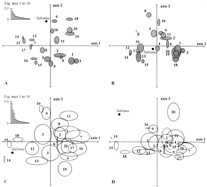
Euclidean distance ordination diagrams based on principal components analysis of the species by their biological attributes (ab) and by physical habitat characteristics (cd). All axis scores are between ‐1 and +1. The attribute groups are located at the centroid (arithmetic mean) of the axis scores of their member species. The ellipses are defined by the standard deviation of the scores from the centroid on each axis. The insets show the pattern of change in eigenvalues.

Multiple discriminant analysis based on the species scores from the initial five axes of this PCA, which summarized 50% of the variation in the attribute data, achieved 92% correct reclassification ( Table 5). Thus, the classification appears to be robust and is suppor‐ted by the PCA ordination.

Table 5.

Results of multiple discriminant analysis using species scores from the initial five axes of principal component analyses to predict group membership. The values given are the percentage of group members correctly reclassified using the axes scores from the stated ordination

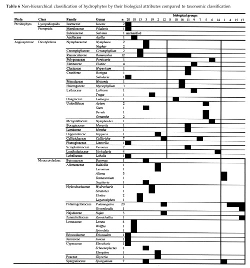
Under partial PCA, 46% of the variance in the trait attribute data was removed by supplying ‘family’ as a co‐variable. Applied to the first five axes of this ordination, MDA achieved a 58% correct reclassification ( Table 5). This suggests that approximately one‐third of the overall classification can be attri‐buted to taxonomic relatedness. The groups which showed the greatest loss in reclassification efficiency relative to that obtained using the unconstrained analysis (1, 5, 9, 14, 16 and 18) were those which contained most or all of the representatives of a particular family (i.e. Alismataceae, Sparganiaceae, Umbelliferae, Elatinaceae, Lentibulariaceae, Haloragaceae and Lemnaceae; Table 6). A few groups contained only a single genus (4, 7, 8, 14 and 15) or family (5), but representatives of the two largest families, Ranunculaceae and Potamogetonaceae, occurred across five and four attribute groups, respectively. The same set of attributes can also clearly be displayed by members of different families (6, 9 and 17) by species from well‐separated orders (1, 10, 11 and 16), by both monocots and dicots (2, 3, 12, 13, 19 and 20), or even by pteridophytes and angiosperms (18 and 20).

Table 6.

Non‐hierarchical classification of hydrophytes by their biological attributes compared to taxonomic classification

Habitat utilization

An ordination of species by their habitat characteristics using PCA identified three major axes of variation which together accounted for 60% of the variation in the habitat data. The results of this PCA are summarized in Fig. 2c,d. The axis scores of the habitat characteristics indicated that axis 1 describes a gradient from standing or sluggish flowing waters, rarely subject to scouring, overlying fine, mixed or organic sediments (e.g. sheltered lakes, bays, ponds, ditches, backwaters and canals) on the left, to moderate‐fast flowing, occasionally or frequently scoured sites, with coarse‐grained mineral substrata and variable sedimentation rates (e.g. rivers in spatey catchments or exposed lake shores). Axis 2 is best regarded as a gradient of increasing temporal heterogeneity from generally deep, stable, rarely disturbed sites (low scores) to shallow, fluctuating and more frequently disturbed habitats. Eleven groups showed reasonable habitat differentiation over the first two axes, while group 20 was separated from the remaining groups on the third axis (shift from habitats with moderate‐high sedimentation rates to coarse‐bedded, rarely disturbed habitats with low sedimentation rates). However, there was a high degree of overlap in habitat use among seven groups (2, 4, 5, 7, 8, 16 and 17) which were associated with more spatially complex environments.

Based on the species scores from the first five axes of the habitat PCA, MDA offers an independent test of the correspondence between attribute groups and the distribution of their members in terms of habitat use. The first five axes of the PCA summarized 71% of the variation in habitat use. Using the species scores from these axes, MDA correctly reclassified 54% of the species into their independently derived attribute groups ( Table 5). Eight groups (4, 6, 10, 11, 14, 17, 19 and 20) achieved a reclassification rate > 66%, but in six groups (2, 3, 5, 7, 8 and 13) where there was high intragroup variation in habitat use and/or high inter group overlap, < 40% of species were correctly reclassified. Axes scores from an ordination of habitat use supplemented by data on habitat fertility ( Table 2) did not improve the rate of reclassification (51%).

Relationships between traits, attribute groups and habitat utilization

Fig. 3 presents the results of RDA in which habitat characteristics are treated as the dependent variable. The analysis explained 72% of the total variation in habitat use. Axes 1 and 2 (eigenvalues = 0.24 and 0.16, respectively) were both significant at P = 0.01 (Monte Carlo unrestricted random permutation test; 999 permutations) and together explained 39% of the total variation. The habitat characteristics best explained (> 75% of variance) were intermediate depth, slow flow rate, occasional scouring, permanent and occasionally temporary water levels, and sand and mineral substratum. Table 7 shows the individual contribution of species attributes to the explanation of variance in habitat use and the intraset correlations between the trait attribute‐derived sample (i.e. species) scores which are a linear combination of the 58 trait attributes (explanatory variables) and the rawattribute data. On the basis of forward selection (variables added to model in order of maximum extra fit) followed by unrestricted permutation tests, twenty‐one out of the 58 trait attributes were significantly correlated (P < 0.05) with habitat utilization. These variables together explained over half (52%) of the total variation in habitat use and 72% of the explainable inertia. The first eight attributes to be selected (i.e. turions, anchored emergent leaves, high body flexibility, high root:shoot biomass ratio, low flexibility, free floating surface and free floating submerged growth forms, and annual life history) accounted for 50% of the explainable inertia. A partial RDA with ‘family’ as the co‐variable showed that 19% of the total variance in habitat use was explained by taxonomy, with 53% being explained by trait attributes independent of the phylogeny of the species.

Figure 3.

Redundancy analysis ordination diagrams depicting the distribution of (a) selected trait attributes and attribute groups, and (b) habitat characteristics. See the text for details. The attribute groups are located at the centroid (arithmetic mean) of the axis scores of their member species. The labels are placed immediately to the right of their scores. Minor adjustments have been made in some cases to avoid overlap.

Table 7.

Correlation coefficients between sample scores which are linear correlations of explanatory variables and individual trait attributes (n = 120), and the independent contribution of trait attributes to an explanation of variance in habitat utilization (total = 0.724) using redundancy analysis. Attributes in bold explained a significant proportion of the residual variance when fitted using forward selection (P < 0.05; Monte Carlo test, 199 random permutations)

By comparing the relative positions of attribute groups, trait attributes and habitat characteristics in Fig. 3 it can be concluded, for example, that the hydrophyte attributes associated most strongly with spatially simple, rarely disturbed habitats (high scores on axis 1) are free‐floating surface or free‐floating submerged growth form, very small body size and turion. These attributes are most prominent in groups 14, 18 and 19 ( Table 4) which include Utricularia spp., Lemna spp. and Hydrocharis morsus‐ranae. The strength of the habitat‐trait relationship, derived directly from the correlation coefficients in the CANOCO 4 species × environment table, means that anchored submerged growth form or tubular leaves are relatively unlikely attributes of the vegetation occurring in this habitat. Other habitat‐trait relationships are summarized in Table 8 using simple groupings of habitat characteristics suggested by Fig. 3 as a framework.

Table 8.

Summary of principal attributes of aquatic vegetation associated with different habitats (expressed as combinations of spatial‐temporal heterogeneity), as derived from a species × environment table produced by RDA

Discussion

Attribute group composition

The growth form classification system of den Hartog & Segal (1964), plus later refinements and extension by Hutchinson (1975) and Wiegleb (1991), is essentially a subjective classification based on morphological characteristics of aquatic plant phenotypes. Since growth form is a morphological expression of a range of physiological and morphological traits ( Grime et al., 1988 ; Montalvo et al., 1991 ; Leishman & Westoby, 1992), some similarities between our attribute groups and growth form classifications were to be expected ( Table 9). Thus, several growth forms, such as the isoetids (group 20), lemnids (18), utricularids (14) and hydrocharids (19) were preserved (previous classifications have sometimes included Salvinia natans with the hydrocharids). However, some attribute groups were composed of multiple and often diverse growth forms (e.g. 1, 2, 3 and 13), while some distinct growth forms occurred across several different attribute groups (e.g. the elodeids and nymphaeids of den Hartog & Segal (1964), the parvopotamid and myriophyllid of Hutchinson (1975), and the magnonymphaeid and pepliden of Wiegleb (1991)). There are several important differences between the two approaches which could account for these discrepancies: (1) we used a wider set of attributes than are strictly relevant to growth form (e.g. some regenerative traits); (2) the clustering method was less subjective, although it may have created some groups of residual heterogenous species perhaps more appropriately considered in isolation (e.g. group 2); (3) growth form plasticity was regarded as a feature of the species complex, and this resulted in a fixed rather than flexible classification of species such as Sagittaria sagittifolia, in which variation in growth form is likely to have a predominantly environmental rather than genetic basis; and (4) we included amphibious species since many produce persistent underwater populations through vegetative reproduction (e.g. Alisma sp. and Elatine sp.).

Table 9.

Comparison between attribute groups and selected growth‐form‐based classifications of hydrophytes

Although attributes related to resource acquisition were largely excluded from our analysis, the classification still reflects underlying correlations between morphology and ecophysiology in isolating the carnivorous bladderworts (group 14), and the isoetids (group 20); the latter incorporate a suite of well‐known ecophysiological adaptations to survive low inorganic carbon availability (e.g. crassulacean acid metabolism, mycorrhizal roots, root foraging for sediment interstitial CO₂, large lacunal air spaces; Farmer & Spence, 1986; Bowes, 1987). The presence of aerial tissue in the form of floating or emergent leaves also provides access to atmospheric CO₂, and sets apart groups 12, 13, 15 and 17 which are exclusively submerged. However, there is experimental evidence of significant within‐group variation in factors including HCO₃ ^‐ affinity (e.g. groups 4 and 16; Maberly & Spence, 1983; Bodner, 1994; Maberly & Madsen, 1998), acidity tolerance (e.g. group 8; Maessen et al., 1992 ) and N‐NH₄ ⁺ tolerance (e.g. groups 4 and 13; Dendene et al., 1993 ) which must reflect adaptations at the cellular level. These are likely to translate to differences in trophic preferences independent of attribute group composition.

Aquatic macrophytes have previously been ‘shoe‐horned’ into Grimes' C‐S‐R classification using selected traits (e.g. Rørslett, 1989; Murphy et al., 1990 ), which it is tentatively assumed, despite the considerable differences in selection pressures in aquatic environments and their multidimensional nature, have a broadly transferable functional role. Some parallels with our groups exist, but we have deliberately avoided the use of strategy labels because these are almost inevitably context‐sensitive ( Smith et al., 1993 ), and thus, potentially misleading when considered out of context. The isoetids (group 20) have often been regarded as the classic stress tolerators of aquatic habitats, in view of attributes such as wintergreenness, small stature, longevity and high below‐ground relative to above‐ground biomass ( Farmer & Spence, 1986; Rørslett, 1989; Boutin & Keddy, 1993), but even within this relatively robust group, some strong ruderal (e.g. Subularia aquatica) or competitor (Juncus bulbosus) affinities exist. Groups 3, 4, 13 and 15 display several typically competitive traits (e.g. high dense canopy, extensive lateral spread, storage of photosynthate as capital for the next season: Grime et al., 1988 ; Kautsky, 1988; Murphy et al., 1990 ), but as Bornette et al. (1994) have pointed out, the lemnids (group 18) can achieve competitive dominance with a markedly different combination of attributes (free‐floating surface tiny leaves; budding). Groups 8, 9, 10 and 11 conform more closely to primary or mixed ruderal strategies, as might be expected of hydrophytes occurring near the interface with terrestrial habitat, but most other groups have no obvious terrestrial analogue. When drawing comparisons with the C‐S‐R classification, it should be borne in mind that hydrophytes exist within a restricted region of the template envisaged for terrestrial vegetation and that the groups recognized may represent variants of a subset of the strategies reported for terrestrial plants. According to Rørslett (1989), for example, most hydrophytes display characteristically stress‐tolerant and/or ruderal traits within the overall context of plant strategies. In this study, we sought to use an attribute data‐set based on intrinsic properties (sensu Steneck & Dethier, 1994) relevant specifically to hydrophytes, i.e. the combination of attributes reflecting the potential expression of the genotype. Thus, our groups do not necessarily possess suites of trait attributes which correspond clearly to the strategies proposed by Grime et al. (1988) or Kautsky (1988). Further attempts to cross‐match classifications are probably of little value since only the finer levels of partitioning (highest level strategies sensu Wiegleb & Brux, 1991) are likely to be of fundamental interest and potential relevance in management and applied ecology ( Abernethy, Sabbatini & Murphy, 1996).

Habitat utilization

The species we considered are dispersed within the habitat PCA and RDA on two strongly opposing axes of spatio‐temporal variation. Given that our attribute‐based classification seems to be robust, if present‐day habitat use is determined by the attributes or combination of attributes which species possess, then we would expect a reasonable match between attribute groups and habitat. While this is true of some groups, the reclassification of species into attribute groups using MDA suggests that, in general, there is only modest correspondence between attribute groups and habitat utilization. This outcome can be attributed to both methodological and underlying ecological factors:

• 1The attribute groups we defined are separated by environmental variables which we did not consider. This seems unlikely because the reclassification of our attribute groups under discriminant analysis was virtually unaffected when we used the axis scores from a habitat PCA incorporating fertility to predict group membership. Improved separation involving a resource gradient is likely to require inclusion of ecophysiological traits in the definition of groups. Nevertheless, some potentially overlapping groups, such as 3 and 13, clearly have access to different resources as a result of the presence or absence of aerial tissue. An associated possibility is that our trait attributes are too coarse‐grained for effective separation of some groups.
• 2The addition of other traits (e.g. other regenerative or phenological traits) or improved resolution of existing traits would give different groupings separated better within the habitat space we defined. Significant changes to our classification would require that new attributes show low covariance with existing attributes, which seems unlikely given the large number of morphological‐regenerative traits which we considered.
• 3Alternative attribute groups, well separated in Fig. 2a,b, can be effective under the same level of spatial‐temporal heterogeneity because of trade‐offs between individual traits ( Wiegleb & Brux, 1991; Townsend & Hildrew, 1994) or the effects of past evolutionary constraints. Some pairs of groups overlap even though within‐group variance in habitat use may be low (9 versus 10, 12 versus 13, 16 versus 17 and 18 versus 19). Leps, Osbornova‐Kosinova & Rejmanek (1982) and MacGillivray et al. (1995) have also noted trade‐offs between resistance and resilience in grassland communities. Contrasting phenology and complementary responses to flooding‐related disturbance in rivers (resistance, through streamlining and fixed depth of rooting, versus population resilience, through rapid growth from vegetative fragments or seeds, and/or intact plants surviving in spatial refugia), could offer a mechanism for coexistence in patchy and temporally heterogenous habitats by Ranunculus fluitans or R. penicillatus (group 16), and Zannichellia palustris and/or Groenlandia densa (group 17), for example. Similarly, contrasting emphasis on propagation via fragmentation and seed production could assist temporal niche partitioning between groups 12 and 13.
• 4Within‐group variation in habitat use is high. This appears to be the main cause of very low rates of correct reclassification (groups 2, 3, 5, 7, 8 and 13). This may be because some borderline species are poorly classified in terms of their traits, or because the trait profile for a group is varied and different traits are important in different parts of the habitat range of the group, but are ‘drowned out’ in classification by a common subset of redundant traits. It could also be because of ‘functional plasticity’ ‐ a common trait or set of traits which can perform different functions, and therefore, is successful in different habitats. For example, group 16 contains several dissected‐leaved species. Hottonia palustris and Myriophyllum verticillatum are typical of standing waters where dissected leaves might enhance gas exchange or uptake of dissolved inorganic carbon (DIC), or reduce self‐shading. By contrast, Ranunculus fluitans and R. penicillatus are typical of moderate to fast‐flowing rivers where diffusion gradients, DIC availability or self‐shading are less significant constraints, but dissected leaves will reduce drag through form reduction. The final members, M. spicatum and M. alterniflorum, occur under both sets of conditions. Similarly, waxy, strap‐shaped floating leaves (e.g. group 1) are responsive to fluctuating water levels, offer protection from desiccation and enable rapid coverage of wet mud if water levels subside, yet also provide effective stream lining in flowing waters. Grace (1993) has further emphasized the variety of functions performed by hydrophyte tissues involved in clonal propagation, in addition to the basic objective of numerical increase. Hence, the rhizomes common to group 3 species could provide effective anchorage in rivers, support through buoyancy and protection from anoxia in semi‐fluid, organic‐rich sediments, as well as contributing significantly to resource storage. Finally, variation in habitat use may be high if group members are linked more strongly by common ancestry than by convergent evolution ( van Groenendael et al., 1996 ). This might apply especially to groups 7 and 8, two monophyletic groups featuring critical taxa (Callitriche and Ranunculus subgenus Batrachium, respectively) in which species are of uncertain origin, poorly separated because of morphological reduction, and therefore, distinguished mainly on the basis of ecologically trivial characteristics, and in the case of group 8, are known to hybridize freely and form persistent sterile or fertile populations ( Cook, 1970).

Redundancy analysis indicates that trait attributes can explain a significant degree of the variation in habitat use. Unfortunately, comparisons with the predictions of Townsend & Hildrew (1994) are partially confounded by an underlying correlation between high spatial heterogeneity and scouring (a source of disturbance in rivers and exposed lake shores) and the dominance of the second axis by water level fluctuations. Thus, the RDA and habitat PCA extract similar axes to those recognized by Cellot et al. (1994) in developing an environmental framework for river floodplain habitats on the Upper Rhôe (i.e. spatial axis based on sediment grain size and organic matter content, and temporal axis based on variation in water depth). This reflects our rather catholic definition of hydrophyte and our ‘global’ view of freshwater habitats. Hence, members of group 12, which are intolerant of desiccation in the established phase but include many typically pioneer species ( Wade, Vanhecke & Barry, 1986; Kautsky, 1988; Wiegleb et al., 1991 ) which recruit rapidly from the seed bank following re‐wetting (as in temporary marshes or rice fields; Grillas, 1990; Triest, 1986), are relegated on the temporal heterogeneity axis by the inclusion of species tolerant of temporary or even permanent exposure. A matrix based exclusively on lacustrine or riverine hydrophytes sensu stricto would probably highlight wave exposure or flood scouring as key temporal influences (e.g. Kautsky, 1988; Bornette et al., 1994 ).

The emphasis on high investment traits, such as large to very large body size, plus low reproductive output, in deep, permanent, slow‐flowing sites with infrequent scouring or disturbance ( Table 8), is consistent with the generally expected shift towards more competitive traits in spatially and temporally uniform habitats. The strong association between temporally variable habitats, and various resilience (small body size, short‐lived perennial life history, high reproductive output, early reproduction and spread by stolons) and resistance type attributes (anchored emergent/heterophyllous leaves, waxy leaves, nodal rooting and the ability to produce a persistent amphibious growth form) is also consistent with predictions. As would be expected in shallow water habitats with fluctuating water levels, life stages susceptible to desiccation are penalized. Several attributes appear to be general features of the vegetation of early successional environments ( Prach et al., 1997 ) and hydrophytes occurring at the land‐water interface (e.g. groups 8, 9, 10 and 11) exhibit many of the classic characteristics of terrestrial ruderals ( Rørslett, 1989). Bornette et al. (1994) also observed that heterophylly, high regeneration potential, reproduction by fragmentation, anchorage and desiccation tolerance were common attributes of hydrophytes in temporally variable floodplain habitats. In the spatially complex, temporally intermediate sites, the emphasis is on resistance traits related to stream lining, anchorage and flexilibility, despite the fact that these habitats are often also temporally heterogenous in terms of susceptibility to scouring or sedimentation. On coarse substrata with low sedimentation rates, an intercorrelation with resource‐poor environments is reflected in attributes such as wintergreeness and inflexible tubular leaves. Large to very large body size and leaf area are high investment attributes expected in more temporally stable habitats, but are clearly compatible with moderate flows and intermittent scouring if combined with high flexibility and/or firm anchorage through rhizomes or nodal rooting. Constant replenishment of waterborne nutrients by flow will also enable rapid repair of damaged tissue.

There is limited support for the hypothesis ( Townsend & Hildrew, 1994) that an increase in refugia in habitats associated with naturally spatially complex environments can ameliorate disturbance to the extent that species lacking resistance/resilience traits are able to survive. This is perhaps because disturbance in the form of desiccation exerts such strong selection pressure on hydrophytes that spatial refugia become effectively irrelevant. However, in the case of disturbance by scouring or sedimentation, river marginal habitats may offer partial refugia for larger species penalized by high hydraulic resistance, such as Nuphar lutea, Sparganium erectum or Potamogeton perfoliatus. Among the isoetids (group 20), short stiff leaves with copious lacunal spaces, high root:shoot biomass and evergreeness are best seen as morphological correlates of ecophysiological adaptations to maximize carbon gain and conserve resources rather than specific adaptations to wave disturbance ( Farmer & Spence, 1986). Indeed, strandline accumulations around oligotrophic lakes suggest that storms may sometimes cause significant mortality of isoetids. Consequently, within those habitats exploited by isoetids, spatial heterogeneity (e.g. variation in water depth or sediment stability) may play an important role in buffering the effects of wave exposure.

There is also clear evidence of an underlying trade‐off between resistance‐type traits (i.e. soft, flexible‐leaved species with a well anchored submerged growth form) in more spatially heterogenous habitats and resilience‐type traits in spatially simple habitats, compatible with the predictions of Grace (1993). We would contend that turions and small body size are primarily features of habitats with few spatial refugia, and which are subject to low‐frequency but high‐magnitude disturbance events (e.g. flood scouring of riverine backwaters, dredging of canals or ditches, or large storm events in lakes) which result in a high mortality of adult plants because of minimal investment in streamlining or anchorage. Since turions offer little protection from prolonged desiccation, this mechanism of clonal propagation is most strongly developed in permanent aquatic habitats. It offers a low‐cost‐high‐output strategy ( Grace, 1993), contributing to rapid population recovery in the wake of disturbance (e.g. Henry, Amoros & Bornette, 1996). The free‐floating nature of adult plants complements this strategy by ensuring rapid water‐borne dispersal and recolonization.

Implications

There is growing interest in freshwater ecology in the use of functional groups or morphological descriptors for predictive purposes. Recent examples include Charvet et al. (1998) and Huszar & Caraco (1998). Previous studies using plant traits to predict hydrophyte responses to environmental change have operated at the species level: Wiegleb et al. (1991) used differences in life‐history attributes to explain changes in the abundance of Potamogeton species in north German rivers in relation to human impacts; Duarte & Roff (1991) used plant architecture and life‐history traits to model the response of lake macrophyte communities to changes in productivity potential; and Henry, Amoros & Bornette (1996) used regenerative traits to predict the order of species re‐establishment in former river channels after flood disturbances. The approach described here enables prediction of general shifts in vegetation attributes with environmental change, or conversely, reconstruction of past environments from known changes in species composition. Predictions might be based on attribute group‐habitat associations or may exploit individual attributes ( Noble & Slatyer, 1980) which explain a large component of variation in habitat use (e.g. highly ranked variables in Table 7). A related option might be to weight trait attributes (e.g. according to their correlation with habitat variables) and reclassify species into ecological groups, followed by testing against an independent matrix of habitat utilization. Testing broad predictions and providing more precise calibration of temporal and spatial axes are essential next steps in a study of this type ( Shipley & Parent, 1991).

Given that hydrophytes span many pronounced gradients of spatial (e.g. light intensity, current velocity and nutrient availability) or temporal environmental variation (e.g. water level fluctuation, flooding and bed movement) ( Kautsky, 1988; Wiegleb & Brux, 1991), relationships between attributes and environment are surprisingly elusive. Perhaps the most enduring is that communities change from low, rosette‐like species to tall, canopy‐forming species dominance along a productivity gradient ( Hutchinson, 1975; Chambers, 1987). Ours and recent studies (e.g. Bornette et al., 1994 ) suggest other possibilities, but there may genuinely be few robust relationships between macrophyte species, traits or attribute groupings and environment. Macrophytes show variable, often high phenotypic plasticity and a wide ecological amplitude, meaning that species‐level attributes which are probably of adaptive value in one part of an ecological range are redundant in other parts and species‐trait‐environment relationships are diluted correspondingly. Trait functional plasticity further limits the potential for strong trait‐environment relationships. Therefore, hydrophyte attribute groups should be used cautiously for habitat assessment or prediction as confidence limits will often be fairly broad.

Our attribute groupings appear to offer an intuitively sensible classification of north‐west European hydrophytes. However, we set out to offer a pragmatic but rigorous approach, not the final word on attribute‐based classification of hydrophytes. Thus, we envisage refinement of these groupings as the relationship between traits and key processes, such as resource acquisition or response to perturbation, is further resolved. Identification of hydrophyte guilds and true functional groups linked to user‐defined functions is then a realistic goal.

Acknowledgments

Considerable thanks are due to J.I. Jones and two anonymous referees for their helpful comments on earlier drafts of this paper. We are also grateful to the Natural Environment Research Council for providing funding during the course of this work, and to K.J. Murphy and other colleagues at Glasgow and previously Liverpool Universities who have contributed to our knowledge, assisted with data collection in the field or supported this work.

(Manuscript accepted 14 July 1999)

References

- Abernethy V.J. (1994). Functional ecology of euhydrophyte communities of European riverine wetland ecosystems.Ph.D. Thesis,University of Glasgow, Glasgow.
- Abernethy V.J., Sabbatini M.R., Murphy K.J. (1996). Response of Elodea canadensis Michx. and Myriophyllum spicatum L. to shade, cutting and competition in experimental culture. Hydrobiologia,340,219 244. [Google Scholar]
- Begon M., Harper J.L., Townsend C.R. (1996). Ecology: Individuals, Populations and Communities.Blackwell Science,Oxford. [Google Scholar]
- Best E.P.H. (1988). The phytosociological approach to the description and classification of aquatic macrophytic vegetation Vegetation of Inland Waters(ed. Symoens J.J.),155 182.Kluwer,Amsterdam. [Google Scholar]
- Biggs J.F., Stevenson R.J., Lowe R.L. (1998). A habitat matrix conceptual model for stream periphyton. Archiv für Hydrobiologie,143,21 56. [Google Scholar]
- Bodner M. (1994). Inorganic carbon source for photosynthesis in the aquatic macrophytes Potamogeton natans and Ranunculus fluitans . Aquatic Botany,48,109 120. [Google Scholar]
- Bornette G., Henry C., Barrat M., Amoros C. (1994). Theoretical habitat templets, species traits and species richness: aquatic macrophytes in the Upper Rhone River and its floodplain. Freshwater Biology,31 487 505. [Google Scholar]
- Botkin D.B. (1975). Functional Groups of organisms in model vegetation Ecosystem Analysis and Prediction(ed. Levin S.A.),98 102.Society for Industrial and Applied Mathematics,Philadelphia, PA. [Google Scholar]
- Boutin C. & Keddy P.A. (1993). A functional classification of wetland plants. Journal of Vegetation Science,4 591 600. [Google Scholar]
- Bowes G. (1987). Aquatic plant photosynthesis: strategies that enhance carbon gain Plant Life in Aquatic and Amphibious Habitats(ed. Crawford R.H.),79 95.Blackwell Scientific Publications,Oxford. [Google Scholar]
- Cellot B., Dole‐Olivier M.J., Bornette G., Pautou G. (1994). Temporal and spatial environmental variability in the upper Rhône River and its floodplain. Freshwater Biology,31,311 325. [Google Scholar]
- Chambers P.A. (1987). Light and nutrients in the control of aquatic plant community structure. II. In situ observations. Journal of Ecology,75,621 628. [Google Scholar]
- Chapin F.S.I., Bret‐Harte M.S., Hobbie S.E., Zhang H. (1996). Plant functional types as predictors of transient responses of arctic vegetation to global change. Journal of Vegetation Science,7,347 358. [Google Scholar]
- Chapleau F., Johansen P.H., Williamson M. (1988). The distinction between pattern and process in evolutionary biology: the use and abuse of the term ‘strategy’. Oikos,53,136 138. [Google Scholar]
- Charvet S., Kosmala A., Statzner B. (1998). Biomonitoring through biological traits of benthic macroinvertebrates: perspectives for a general tool in stream management. Archiv für Hydrobiologie,142,415 432. [Google Scholar]
- Chevenet F., Dolédec S., Chessel D. (1994). A fuzzy coding approach for the analysis of long‐term ecological data. Freshwater Biology,31,295 309. [Google Scholar]
- Cook C.D.K. (1970). Hybridization in the evolution of Batrachium . Taxon,19,161 166. [Google Scholar]
- Cook C.D.K. (1990). Aquatic Plant Book.SPB Academic Publishing,the Hague. [Google Scholar]
- Day R.T., Keddy P.A., McNeill J., Carelton T. (1988). Fertility and disturbance gradients: a summary model for riverine marsh vegetation. Ecology,69,1044 1054. [Google Scholar]
- Dendene M.A., Rolland T., Tremolieres M., Carbiener R. (1993). Effect of ammonium‐ions on the net photosynthesis of 3 species of Elodea . Aquatic Botany,46,301 315. [Google Scholar]
- Diaz S. & Cabido M. (1997). Plant functional types and ecosytem function in relation to global change. Journal of Vegetation Science,8,463 474. [Google Scholar]
- Du Rietz G.E. (1931). Life‐forms of terrestrial flowering plants. Acta Phytogeographica Suecica,3,1 95. [Google Scholar]
- Duarte C.M. & Roff D.A. (1991). Architectural and life history constraints to submersed macrophyte community structure: a simulation study. Aquatic Botany,42,15 29. [Google Scholar]
- Farmer A.M. & Spence D.H.N. (1986). The growth strategies and distribution of isoetids in Scottish freshwater lochs. Aquatic Botany,26,247 258. [Google Scholar]
- Fernandez Ales R., Laffarga J.M., Ortega F. (1993). Strategies in Mediterranean grassland annuals in relation to stress and disturbance. Journal of Vegetation Science,4,313 322. [Google Scholar]
- Fitter A.H. & Peat H.J. (1994). The Ecological Flora Database. Journal of Ecology,82,415 425. [Google Scholar]
- Friedel M.H., Bastin G.N., Griffin G.F. (1988). Range assessment and monitoring in arid lands:the derivation of functional groups to simplify data. Journal of Environmental Management,27,85 97. [Google Scholar]
- Gauch H.G. (1982). Multivariate Analysis in Community Ecology.Cambridge University Press,Cambridge. [Google Scholar]
- Gaudet C.L. & Keddy P.A. (1988). A comparative approach to predicting competitive ability from plants traits. Nature,334,242 243. [Google Scholar]
- Golluscio R.A. & Sala O.E. (1993). Plant functional types and ecological strategies in Patagonian forbes. Journal of Vegetation Science,4,839 846. [Google Scholar]
- Gordon A.D. (1981). Classification: Methods for the Exploratory Analysis of Multivariate Data.Chapman and Hall,London. [Google Scholar]
- Grace J.B. (1993). The adaptive significance of clonal reproduction in angiosperms: an aquatic perspective. Aquatic Botany,44,159 180. [Google Scholar]
- Grillas P. (1990). Distribution of submerged macrophytes in the Camargue in relation to environmental factors. Journal of Vegetation Science,1,393 402. [Google Scholar]
- Grime J.P. (1977). Evidence for the existence of three primary strategies in plants and its relevance to ecological and evolutionary theory. American Naturalist,111,1169 1194. [Google Scholar]
- Grime J.P. (1979). Plant Strategies and Vegetation Processes.John Wiley & Sons,Chichester. [Google Scholar]
- Grime J.P. (1997). Biodiversity and ecosystem function: the debate deepens. Science,277,1260 1261. [Google Scholar]
- Grime J.P., et al. (1997). Integrated screening validates primary axes of specialisation in plants. Oikos,79,259 281. [Google Scholar]
- Grime J.P., Hodgson J.G., Hunt R. (1988). Comparative Plant Ecology.Unwin Hyman,London. [Google Scholar]
- Van Groenendael J.M., Klime L., Klimeová J., Hendriks R.J.J. (1996). Comparative ecology of clonal plants. Philosophical Transactions of the Royal Society London, B,351,1331 1339. [Google Scholar]
- Den Hartog C. & Segal S. (1964). A new classification of the water‐plant communities. Acta Botanica Neerlandica,13,367 393. [Google Scholar]
- Den Hartog C. & Van Der Velde G. (1988). Structural aspects of aquatic plant communities.Vegetation of Inland Waters; (ed. Symoens J.J.),113 153.Kluwer, Amsterdam. [Google Scholar]
- Harvey P.H., Read A.F., Nee S. (1995). Why ecologists need to be phylogenetically challenged. Journal of Ecology,83,535 536. [Google Scholar]
- Henry C.P., Amoros C., Bornette G. (1996). Species traits and recolonisation processes after flood disturbances in riverine macrophytes. Vegetatio,122,13 27. [Google Scholar]
- Hill M.O. (1979). twinspan ‐ A fortran Program for Arranging Multivariate Data in an Ordered Two‐way Table by Classification of the Individuals and Attributes.Cornell University,Ithaca, NY. [Google Scholar]
- Hogeweg P. & Brenkert‐van Riert A.L. (1969). Structure and aquatic vegetation in India, the Netherlands and Czechoslovakia. Tropical Ecology,10,139 162. [Google Scholar]
- Hunt R. & Bossard C.C. (1993). Quantitative synthesis Methods in Comparative Plant Ecology: A Laboratory Manual Hendry G.A.F. and Grime J.P.),223 238.Chapman and Hall,London. [Google Scholar]
- Huszar V.L. de M. & Caraco N.F. (1998). The relationship between phytoplankton composition and physical‐chemical variables: a comparison of taxonomic and morphological‐functional descriptors in six temperate lakes. Freshwater Biology,40,679 696. [Google Scholar]
- Hutchinson G.E. (1975)A Treatise on Limnology,Vol. III:Limnological Botany.John Wiley & Sons,Chichester. [Google Scholar]
- Jongman R.H.G., Ter Braak C.J.F., Van Tongeren O.F.R. (1995). Data Analysis in Landscape and Community Ecology.Cambridge University Press,Cambridge. [Google Scholar]
- Kautsky L. (1988). Life strategies of aquatic soft‐bottom macrophytes. Oikos,53,126 135. [Google Scholar]
- Keddy P.A. (1989). Competition.Chapman and Hall,London. [Google Scholar]
- Keddy P.A. (1992). A pragmatic approach to functional ecology. Functional Ecology,6,621 626. [Google Scholar]
- Kindscher K. & Wells P.V. (1995). Prairie plant guilds: a multivariate analysis of prairie species based on cological and morphological traits. Vegetatio,117,29 50. [Google Scholar]
- Korner C. (1993). Scaling from species to vegetation: the usefulness of functional groups Biodiversity and Ecosystem Function Shulze E.D. and Mooney H.A.),117 140.Springer‐Verlag,Berlin. [Google Scholar]
- Krzanowski W.J. (1988). Principles of Multivariate Analysis A User's Perspective.Oxford University Press,Oxford. [Google Scholar]
- Krzanowski W.J. & Lai Y.T. (1988). A criterion for determining the number of groups in a data set sum‐of‐squares clustering. Biometrics,44,23 34. [Google Scholar]
- Leishman M.R. & Westoby M. (1992). Classifying plants into groups on the basis of individual traits ‐ evidence from Australian semi‐arid woodlands. Journal of Ecology,80,417 424. [Google Scholar]
- Leps J., Osbornova‐Kosinova J., Rejmanek M. (1982). Community stability, complexity and species life‐history strategies. Vegetatio,50,53 63. [Google Scholar]
- Lincoln R.J., Boxshall G.A., Clark P.F. (1982). A Dictionary of Ecology, Evolution and Systematics.Cambridge University Press,Cambridge. [Google Scholar]
- Maberly S.C. & Madsen T.V. (1998). Affinity for CO2 in relation to the ability of freshwater macrophytes to use HCO3 ‐ . Functional Ecology,12,99 106. [Google Scholar]
- Maberly S.C. & Spence D.H.N. (1983). Photosynthetic inorganic carbon use by freshwater plants. Journal of Ecology,71,705 724. [Google Scholar]
- MacGillivray C.W. & Grime J.P.&the I.S.P. team (1995). Testing predictions of resistance and resilience of vegetation subjected to extreme events. Functional Ecology,9,640 649. [Google Scholar]
- Maessen M., Roelofs J.G.M., Bellemakers M.J.S., Verheggen G.M. (1992). The effects of aluminium, aluminium‐calcium ratios and pH on aquatic plants from poorly buffered environments. Aquatic Botany,43,115 127. [Google Scholar]
- Montalvo J., Casado M.A., Levassor C., Pineda F.D. (1991). Adaptation of ecological systems: compositional patterns of species and morphological and functional traits. Journal of Vegetation Science,2,655 666. [Google Scholar]
- Moore A.D. & Noble I.R. (1990). An individualistic model of vegetation stand dynamics. Journal of Environmental Management,31,61 81. [Google Scholar]
- Muotka T. & Virtanen R. (1995). The stream as a habitat templet for bryophytes: species distributions along gradients in disturbance and substratum heterogeneity. Freshwater Biology,33,141 160. [Google Scholar]
- Murphy K.J., Castella E., Clement B., Hills J.M., Obrdlik P., Pulford I.D., Schneider E., Speight M.C.D. (1994). Biotic indicators of riverine wetland ecosystem functioning Global Wetlands: Old World and New(ed. Mitsch W.J.),659 682.Elsevier Science,Amsterdam. [Google Scholar]
- Murphy K.J., Rørslett B., Springuel I. (1990). Strategy analysis of submerged lake macrophyte communities: an international example. Aquatic Botany,36,303 323. [Google Scholar]
- Noble I.R. & Slatyer R.O. (1980). The use of vital attributes to predict successional changes in plant communities subject to recurrent disturbances. Vegetatio,43,5 21. [Google Scholar]
- Payne R.W. & Lane P.W.&the Genstat 5 Committee (1993). Genstat 5 Release 3 Reference Manual.Clarendon Press,Oxford. [Google Scholar]
- Prach K., Pysek P., Šmilauer P. (1997). Changes in species traits during succession: a search for pattern. Oikos,79,201 205. [Google Scholar]
- Preston C.D. (1995). Pondweeds of Great Britain and Ireland.Botanical Society of the British Isles,London. [Google Scholar]
- Preston C.D. & Croft J.M. (1997). Aquatic Plants in Britain and Ireland.Harley Books,Colchester. [Google Scholar]
- Raunkiaer (1934). The Life Forms of Plants and Statistical Plant Geography.Clarendon Press,Oxford. [Google Scholar]
- Richards C., Haro R.J., Johnson L.B., Host G.E. (1997). Catchment and reach scale properties as indicators of macroinvertebrate species traits. Freshwater Biology,37,219 230. [Google Scholar]
- Rørslett B. (1989). An integrated approach to hydropower impact assessment. II. Submerged macrophytes in some Norwegian hydro‐electric lakes. Hydrobiologia,175,65 82. [Google Scholar]
- Scarsbrook M.R. & Townsend C.R. (1994). Stream community structure in relation to spatial and temporal variation: a habitat templet study of two contrasting New Zealand streams. Freshwater Biology,29,395 410. [Google Scholar]
- Segal S. (1968). Ein Einteilungsversuch der Wasserpflanzengesellshaften Planzensoziologische Systematik(ed. Tuxen R.),191 219.Junk Publishers,the Hague. [Google Scholar]
- Shipley B. & Keddy P.A. (1988). The relationship between relative growth rate and sensitivity to nutrient stress in 28 species of emergent macrophytes. Journal of Ecology,76,1101 1110. [Google Scholar]
- Shipley B., Keddy P.A., Moore D.R.J., Lemky K. (1989). Regeneration and establishment strategies of emergent macrophytes. Journal of Ecology,77,1093 1110. [Google Scholar]
- Shipley B. & Parent M. (1991). Germination response of 64 wetland species in relation to seed size, minimum time to reproduction and seedling relative growth rate. Functional Ecology,5,111 118. [Google Scholar]
- Smith B., Mark A.F., Wilson J.B. (1995). A functional analysis of New Zealand alpine vegetation: variation in canopy roughness and functional diversity in response to an experimental wind barrier. Functional Ecology,9,904 912. [Google Scholar]
- Smith T.M., Shugart H.H., Woodward F.I.(eds)(1997). Plant Functional Types: Their Relevance to Ecosystem Properties and Global Change IGBP Series,Cambridge University Press,Cambridge. [Google Scholar]
- Smith T.M., Shugart H.H., Woodward F.I., Burton P.J. (1993). Plant functional types Vegetation Dynamics and Global Change Solomon A.M. and Shugart H.H.),272 292.Chapman and Hall,London. [Google Scholar]
- Southwood T.R.E. (1977). Habitat: the templet for ecological strategies? Journal of Animal Ecology,46,337 365. [Google Scholar]
- Southwood T.R.E. (1988). Tactics, strategies and templets. Oikos,52,3 18. [Google Scholar]
- Spink A.J. (1992). The ecological strategies of aquatic Ranunculus species .Ph.D. Thesis,University of Glasgow, Glasgow.
- Stace C. (1991). New Flora of the British Isles.Cambridge University Press,Cambridge. [Google Scholar]
- Statzner B., Hoppenhaus K., Arens M., Richoux P. (1997). Reproductive traits, habitat use and templet theory: a synthesis of world‐wide data on aquatic insects. Freshwater Biology,38,109 135. [Google Scholar]
- Statzner B., Resh V.H., Roux A.L. (1994). The synthesis of long term ecological theory: design of a research strategy for the upper Rhône River and its floodplain. Freshwater Biology,31,253 263. [Google Scholar]
- Stearns S.C. (1976). Life history tactics: a review of the ideas. Quarterly Review of Biology,51,3 47. [DOI] [PubMed] [Google Scholar]
- Steneck R.S. & Dethier M.N. (1994). A functional group approach to the structure of algal dominated communities. Oikos,69,476 498. [Google Scholar]
- Ter Braak C.J.F. & Šmilauer P. (1998)Canoco Reference Manual and User's Guide to Canoco for Windows: Software for Canonical Community Ordination (Version 4).Microcomputer Power,Ithaca, NY. [Google Scholar]
- Thompson K., Bakker J., Bekker R. (1997). The Soil Seed Banks of North Western Europe.Cambridge University Press,Cambridge. [Google Scholar]
- Townsend C.R., Doledec S., Scarsbrook M.R. (1997). Species traits in relation to temporal and spatial heterogeneity in streams: a test of habitat templet theory. Freshwater Biology,37,367 387. [Google Scholar]
- Townsend C.R. & Hildrew H.G. (1994). Species traits in relation to a habitat templet for river systems. Freshwater Biology,31,265 275. [Google Scholar]
- Triest L. (1986). Najas L. species (Najadaceae) as rice field weeds 7th International Symposium on Aquatic Weeds,357 362.European Weed Research Society,Loughborough. [Google Scholar]
- Tutin T.G., Heywood V.H., Burges N.A., Moore D.M., Valentine D.H., Walters S.M., Webb D.A.(eds)(19641980). Flora Europeaea.Cambridge University Press,Cambridge. [Google Scholar]
- Wade P.M., Vanhecke L., Barry R. (1986). The importance of habitat creation, weed management and other habitat disturbance to the conservation of the rare aquatic plant, Callitriche truncata Guss. subsp occidentalis (Ruoy) Schotsm 7th International Symposium on Aquatic Weeds,389 394.European Weed Research Society,Loughborough. [Google Scholar]
- Wiegleb G. (1991). Die Lebens‐ und Wuchsformen der Makrophytischen Wasserpflanzen und deren Beziehungen zur Okologie, Verbreitung und Vergesellschaftung der Arten. Tuexenia,11,135 147. [Google Scholar]
- Wiegleb G. & Brux H. (1991). Comparison of life history characters of broad‐leaved species of the genus Potamogeton L. I. General characterisation of morphology and reproductive strategies. Aquatic Botany,39,131 146. [Google Scholar]
- Wiegleb G., Brux H., Herr W. (1991). Human impact on the ecological performance of Potamogeton species in Northern Germany. Vegetatio,97,161 172. [Google Scholar]
- Woodward F.I. & Cramer W. (1996). Plant functional types and climatic change: introduction. Journal of Vegetation Science,7,306 308. [Google Scholar]