Circuit Stability to Perturbations Reveals Hidden Variability in the Balance of Intrinsic and Synaptic Conductances

Abstract

Neurons and circuits each with a distinct balance of intrinsic and synaptic conductances can generate similar behavior but sometimes respond very differently to perturbation. Examining a large family of circuit models with non-identical neurons and synapses underlying rhythmic behavior, we analyzed the circuits' response to modifications in single and multiple intrinsic conductances in the individual neurons. To summarize these changes over the entire range of perturbed parameters, we quantified circuit output by defining a global stability measure. Using this measure, we identified specific subsets of conductances that when perturbed generate similar behavior in diverse individuals of the population. Our unbiased clustering analysis enabled us to quantify circuit stability when simultaneously perturbing multiple conductances as a nonlinear combination of single conductance perturbations. This revealed surprising conductance combinations that can predict the response to specific perturbations, even when the remaining intrinsic and synaptic conductances are unknown. Therefore, our approach can expose hidden variability in the balance of intrinsic and synaptic conductances of the same neurons across different versions of the same circuit solely from the circuit response to perturbations. Developed for a specific family of model circuits, our quantitative approach to characterizing high-dimensional degenerate systems provides a conceptual and analytic framework to guide future theoretical and experimental studies on degeneracy and robustness.

SIGNIFICANCE STATEMENT Neural circuits can generate nearly identical behavior despite neuronal and synaptic parameters varying several-fold between individual instantiations. Yet, when these parameters are perturbed through channel deletions and mutations or environmental disturbances, seemingly identical circuits can respond very differently. What distinguishes inconsequential perturbations that barely alter circuit behavior from disruptive perturbations that drastically disturb circuit output remains unclear. Focusing on a family of rhythmic circuits, we propose a computational approach to reveal hidden variability in the intrinsic and synaptic conductances in seemingly identical circuits based solely on circuit output to different perturbations. We uncover specific conductance combinations that work similarly to maintain stability and predict the effect of changing multiple conductances simultaneously, which often results from neuromodulation or injury.

Introduction

The intrinsic and synaptic conductances in diverse neural circuits, ranging from central pattern generating circuits in invertebrates (Marder and Goaillard, 2006; Schulz et al., 2006; Tobin et al., 2009), to central circuits in mammalian brains (Swensen and Bean, 2005; Günay et al., 2008), can vary several-fold and still generate nearly identical activity patterns. This degeneracy is due to the extensive overlap that ion channels display in their biophysical properties and how they shape neural activity (Marder and Tang, 2010). Although multiple circuits generate similar activity patterns under normal conditions, they can respond very differently when perturbed. One example is the pyloric circuit in the stomatogastric ganglion of crustaceans, which normally generates a stereotypical rhythmic pattern of activity (Tang et al., 2010; Haddad and Marder, 2018). Following extreme temperature perturbations, the circuits in each preparation display so-called “crashes” in different ways, affecting all circuit components (Robertson and Money, 2012; Tang et al., 2012; Rinberg et al., 2013). Yet, in such circuits, some types of perturbations affect individual aspects of circuit output (Ransdell et al., 2013; Sakurai et al., 2014) and can be used to reveal differences in the circuit's intrinsic and synaptic conductances. Beyond rhythmic circuits, degeneracy is also observed during neuropathic pain in primary afferents of nerve-injured rats (Ratté et al., 2014; Ratté and Prescott, 2016).

Given this degeneracy in a circuit's intrinsic and synaptic conductances, many studies have examined how to reliably modulate circuit output while maintaining robustness (Marder et al., 2014). However, experimentally, it is more difficult to record all circuit components over time, compared with a single measure of circuit output. To address this challenge, we used computational modeling where we can read out the values of all biological components and examine how they interact. Unlike previous modeling work, which studied few circuits as representative examples with a desired response (Grashow et al., 2009, 2010; Dethier et al., 2015), we incorporated intrinsic and synaptic biophysical variability in an ensemble modeling approach (Prinz et al., 2004; Lamb and Calabrese, 2013). Specifically, we studied a family of degenerate models of half-center oscillators, small central pattern generating circuits of two neurons coupled with recurrent inhibition (Brown, 1911), a common circuit motif underlying rhythmic behaviors such as breathing and locomotion (Perkel and Mulloney, 1974; Wang and Rinzel, 1992; Sharp et al., 1996). Although modeling studies typically assume identical neurons and synapses, experiments highlight the impact of their variability on circuit output and the circuits' ability to cope with perturbations (Sharp et al., 1996; Grashow et al., 2009, 2010). Therefore, we studied a large population of degenerate half-center circuits composed of non-identical neurons and synapses with properties from the stomatogastric nervous system (Golowasch and Marder, 1992; Liu et al., 1998; Goldman et al., 2001).

We took a novel approach opposite from studies that assumed experimentally observed relationships between the circuits' building blocks. By examining circuit output in response to perturbations, fully or partially blocking or enhancing a given ion channel, we identified surprising conductance combinations that can predict the response to specific perturbations, even when the remaining intrinsic and synaptic conductances are unknown. We first defined a concise measure of circuit stability when altering conductances in biologically plausible ranges based on how significantly circuit output was modified for the entire population of circuits. Unbiased clustering of stability exposed specific subsets of conductances whose perturbation had a similar effect on the output of many degenerate circuits with similar behavior. Unlike classical sensitivity analysis (Goldman et al., 2001; Olypher and Calabrese, 2007; Weaver and Wearne, 2008; Drion et al., 2015), our measure is non-local and goes beyond a linear approximation of the covariation of interacting conductances. We demonstrate this by explaining the stability to perturbations in two conductances simultaneously from the combination of single perturbations, which is relevant for many neuromodulators that alter more than one conductance. Although implemented on a particular family of circuits, our approach provides a broader framework for studying degeneracy and robustness quantitatively, which has the potential to inspire future experimental investigation of these phenomena.

Materials and Methods

Single neuron model

For the dynamics of single neurons, we used Hodgkin–Huxley models with seven different channel types (Fig. 1): fast Na⁺ (Na), fast transient K⁺ (A), Ca²⁺-dependent K⁺ (KCa), a delayed rectifier K⁺ (Kd), a hyperpolarization-activated inward cation current (H) and fast transient Ca²⁺ (CaT) and slow Ca²⁺ (CaS). The transient calcium conductance, CaT, has a faster time constant than the slow CaS, especially for the closing gating variable. Therefore, this conductance increases rapidly when the cell becomes depolarized, and afterward vanishes rapidly. In contrast, during depolarization CaS increases more slowly than CaT, and afterward persists for longer.

Figure 1.

Generating a population of degenerate Hodgkin-Huxley neurons. A, Maximum conductances for different ion channel types were chosen randomly and independently from a uniform range of values (left) to create a population of 750 single neurons with variable firing properties (right). B, Different sets of maximum conductances (left) can produce the same output (right).

Parameter values for the channel dynamics, including activation and inactivation time constants and voltage dependencies, were chosen to capture rhythmic activity of the lateral pyloric neuron in the stomatogastric ganglion of Cancer borealis (Liu et al., 1998) based on experimental work (Golowasch and Marder, 1992):

The capacitance was set to c = 1, the membrane potential was V and each current (I_i) was described by the maximum conductance value ${\overline{\text{g}}}_i$, the reversal potential E_i, and the opening and closing variables m_i and h_i and the integers p_i and q_i. For the leak current, m and h were set to 1 and g_leak = 0.01 µS. The reversal potentials E_leak = –50 mV, E_Na = 50 mV, E_K = –80 mV and E_H = –20 mV were kept fixed, whereas the reversal potential for the calcium-dependent channels was dynamically computed by using the Nernst equation with an extracellular Ca²⁺ concentration of 3 mM following Liu et al. (1998) for the sake of consistency with the other parameters, although the extracellular Ca²⁺ concentration in the crab is 13 mM (Golowasch et al., 1999; Zhang and Golowasch, 2007). The intracellular Ca²⁺ concentration depended on the influx of Ca²⁺ through the Ca²⁺-dependent channels, as well as on a linear buffer rate:

with a time constant ${\tau }_{\text{Ca}}=200$ ms. The opening and closing parameters were modeled by the following equations (where we omitted the subscript i on m and h for clarity):

To build single neuron models we selected the maximum conductance values (in µS) from the following ranges: ${\overline{g}}_{\text{Na}}\in \left[800,1200\right],\hspace{0.17em}{\overline{g}}_{\text{CaT}}\in \left[0,6\right],\hspace{0.17em}{\overline{g}}_{\text{CaS}}\in \left[0,12\right],\hspace{0.17em}{\overline{g}}_{\text{A}}\in \left[20,130\right],\hspace{0.17em}{\overline{g}}_{\text{KCa}}\in \left[20,140\right],\hspace{0.17em}{\overline{g}}_{\text{Kd}}\in \left[90,120\right],\hspace{0.17em}{\overline{g}}_{\text{H}}\in \left[0,2\right]$.

Half-center circuit model

To generate half-center circuits (Fig. 2), two cells were coupled via a graded synaptic connection (Graubard et al., 1980; Johnson et al., 1995) where the synaptic input current I_syn adds an additional input to Equation 1 for the postsynaptic cell (Cell 1) and depends on the membrane voltage of the presynaptic cell (Cell 2) $V^{\ast }$ (Golomb et al., 1994):

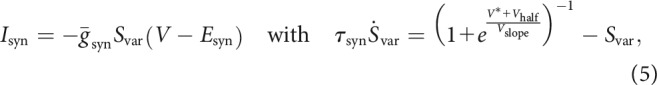with V_half = 45 mV, V_slope = –2 mV, ${\tau }_{\text{syn}}=100$ ms and E_syn = –78 mV. Here, ${\overline{g}}_{\text{syn}}={\overline{g}}_{\text{21}}$ denotes the connection from Cell 1 to Cell 2. Similarly, the reciprocal connection from Cell 2 to Cell 1 is ${\overline{g}}_{\text{syn}}={\overline{g}}_{\text{12}}$. To determine synaptic strengths that generate a specific output, we scanned the space of all possible synaptic connections in a Monte Carlo fashion as follows. For each randomly selected pair of neurons, we chose a pair of synaptic conductances from a grid in the range [0,1] µS with a resolution of 0.025 µS. To introduce variability in an unbiased fashion, we further added jitter to each conductance from the range [–0.0125, 0.0125] µS with a resolution of 0.0025 µS. Each potential circuit was simulated for 4.5 s. We efficiently sampled the entire space of synaptic conductances using a batch approach; performing 32 circuit simulations per batch, we evaluated the output of each circuit. If Cell 1 suppressed Cell 2 for a specific pair of synaptic conductances, we observed that Cell 1 continued suppressing Cell 2 when further increasing the synaptic connection from Cell 1 to Cell 2 (${\overline{g}}_{\text{21}}$). Thus, we excluded all bigger synaptic conductances from the remaining selection process after each batch. We call this Monte Carlo process “self-refining”.

Figure 2.

Generating a population of degenerate half-center circuits (HCCs). A, Three circuit behaviors are possible when reciprocally connecting two neurons via inhibitory synapses: one of the cells is silent (red cross), both cells are active but the circuit does not satisfy all three of the criteria (see text) for a functional circuit (yellow circle), and both cells are active and the circuit satisfies all three of the criteria for a functional circuit (green circle). ϕ Denotes the phase difference between the two cells in the circuit as a fraction of the circuit period. B, The type of HCCs built from three different randomly chosen pairs of neurons where the synaptic conductances were varied in a two-dimensional grid. Depending on the neuron pair, functional HCCs result when one synaptic conductance is greater than the other (left), when the two synaptic conductances have similar strength (middle), or for no choice of synaptic conductances (right). For every pair of neurons, instead of testing the output of a given circuit for every pair of synaptic conductances, we stopped searching for synaptic conductances bigger than a value that rendered one cell silent and when there were at least three functional circuits (green circles); here we show all identified functional circuits for completeness (Methods). Some neuron pairs yielded larger sets of solutions (e.g., middle). C, Different sets of maximum intrinsic and synaptic conductances (left) lead to the same circuit behavior (right).

During this self-refining random sampling, we observed three different outcomes of circuit output: (1) the circuit is considered “functional” when both cells are active, fire regularly and in alternation with a phase difference, period and burst exclusion metric as defined in the main text (Fig. 2A,B, green circles), (2) both cells are active but they do not fulfill the requirements for the circuit to be considered functional: although they fire in alternation, they do not have the phase difference, period and burst exclusion matrix that we require (Fig. 2A,B, yellow circles), or (3) one of the cells is silent (Fig. 2A,B, red crosses). The random sampling was terminated when the circuit output evaluation generated at least three functional circuits (though in Fig. 2B we did not terminate the scan for the purpose of visualization), or if the whole grid of synaptic conductances generated no functional circuit output. In our analysis, we used only one of the three functional circuits for each pair of neurons and synaptic conductances.

In summary, our population generation protocol can be described as follows. We started with 750 single neurons. These could be combined into a total of 281,625 pairs, allowing us to form a total of 450,600,000 possible circuits because each pair could be combined into a circuit with 1600 different possible synaptic connections. We scanned all pairs and found a surprisingly large number, approximately half of them (137,028), which could form circuits that satisfy our conditions. In particular, we scanned a total of ∼300 million possible circuits made by these pairs, based on the self-refining procedure. Because of time and computational constraints, we finally randomly selected 7690 circuits for our detailed analysis. The functional circuits were further simulated for a longer period of 120 s to ensure that their regular firing properties persisted.

Burst detection

During each simulation, an event was counted as a spike when the membrane voltage of the neuron crossed the threshold of −30 mV from below. To extract bursts, we applied a threshold to the interspike intervals (ISIs) that was determined by one-half the sum of 90th percentile of the whole spike train ISI distribution and the minimal ISI. When this threshold was too close to the maximum or minimum values of the ISI (<10 ms), the cell was considered to spike. For coupled cells, all bursts of one cell that occurred between bursts or spikes of the other cell in the circuit were considered one long burst.

In addition, we used the burst exclusion metric x_network (Grashow et al., 2009) to determine whether the bursts fired in an alternating fashion (x_network = 1). The metric is computed by calculating the total active time of both cells (t_cell1 and t_cell2) and the overlap of both cells being active at the same time in the circuit (O_network). The latter is compared with the overlap time that would happen randomly for uncorrelated cells (O_random) and the minimum possible overlap time (O_min) during the total simulation time T_trial:

Stability value

For each circuit we determined the initial unperturbed phase difference ϕ₀, defined as the time between the onset of a burst from one cell to the onset of the next burst of the other cell divided by the period of the circuit. This also included bursts consisting of just a single spike. We perturbed the circuit in N = 15 steps (in each direction for increases and decreases) and for each step i extracted the resulting phase difference ϕ_i. Then we can calculate the proximity of the phase difference ϕ_i to the initial phase difference ϕ₀:

The stability value θ is defined as the average proximity over all perturbation steps (Fig. 4):

Figure 4.

Quantifying circuit stability in response to intrinsic conductance perturbations. A, Definition of the stability value to single conductance perturbations. (1) One cell is perturbed by changing one of its intrinsic conductances in 30 steps between 0 and 200%. (2) For each perturbation, the new phase difference of the perturbed circuit output is computed. (3) The new phase difference is compared with the phase difference of the unperturbed circuit: a proximity of 0 indicates a large difference (or one cell is silent), whereas a proximity of 1 indicates a phase difference the same as the initial. Finally, the stability value $\theta \in [0,1]$ is the average proximity of all perturbed circuits. Two different stability values concisely describe the change in phase difference for decreases (↓) versus increases (↑) in the maximum conductance. B, Stability values when perturbing ${\overline{g}}_{\text{CaS}}$ and ${\overline{g}}_{\text{H}}$ in the same circuit.

Influence of the unperturbed cell on stability

To determine how specific circuit attributes correlate with circuit stability in response to conductance perturbations in circuits with an identical perturbed cell, we chose a total of 100 subsets, each consisting of 18–29 circuits, for a total of 2002 circuits (Fig. 5). For every subset, we selected one perturbation (e.g., an increase in ${\overline{g}}_{\text{CaT}}$) to calculate the Spearman correlation coefficient between the stability value (e.g., ${\theta }_{\text{CaT}\uparrow }$) and an attribute of either the unperturbed cell when uncoupled or an attribute of the unperturbed circuit (e.g., the synaptic connection to the perturbed cell; Fig. 5). We then evaluated the statistical significance of these correlations.

Figure 5.

Diverse stability values in response to different intrinsic conductance perturbations. A, Top, A schematic illustrating a subset of circuits with the same perturbed cell (red) and distinct unperturbed cells (gray). Middle, The output of each cell when uncoupled, to illustrate the feature “period of the unperturbed cell”. Bottom, The output of the circuit. B–D, The gray histograms show the distribution of stability of all 7690 circuits for different perturbations, ${\theta }_{\text{CaT}\uparrow },\hspace{0.17em}{\theta }_{\text{CaS}\downarrow }$ and ${\theta }_{\text{H}\downarrow }$. In addition, the right ordinate axis shows: (B) the relationship between the synaptic conductance to the perturbed cell (${\overline{g}}_{\text{12}}$; A, bottom) and the stability values ${\theta }_{\text{CaT}\uparrow },\hspace{0.17em}{\theta }_{\text{CaS}\downarrow }$ and ${\theta }_{\text{H}\downarrow }$ (symbols) for 20 different circuits with the same perturbed cell and distinct unperturbed cells; (C) the relationship between the synaptic conductance to the unperturbed cell (${\overline{g}}_{\text{21}}$; A, bottom) and the same stability values; (D) The relationship between the period of the unperturbed cell when uncoupled (A, middle) and the same stability values. In each case, the Spearman correlation coefficient and p-value are provided. E, Boxplots show the median and the quartiles of all correlation coefficients for 100 subsets of circuits (2002 circuits total), each subset with the same perturbed cell and with 18–29 distinct unperturbed cells. The whiskers are extended to 1.5 of the interquartile range and black diamonds indicate outliers outside this range. The statistically significant correlations (p < 0.05) from these subsets are superimposed as gray circles. The numbers indicate the number of subsets from those 100 with a statistically significant Spearman correlation coefficient, whereas the red asterisks indicate the single subset of 20 circuits from B through D. Only correlations between ${\theta }_{\text{CaT}\uparrow },\hspace{0.17em}{\theta }_{\text{CaS}\downarrow }$ and ${\theta }_{\text{H}\downarrow }$ and three circuit features (${\overline{g}}_{\text{12}},\hspace{0.17em}{\overline{g}}_{\text{21}}$ and period of unperturbed cell) are shown.

Statistical analysis

The significance of the Spearman correlation was determined using the scipy function scipy.stats.spearmanr. Because the analysis is repeated 100 times, for a significance value of p < 0.05 we expect to see $\sim 5$ significant correlations by chance, even with uncorrelated datasets.

Hierarchical clustering algorithm

The hierarchical clustering algorithm (Fig. 6) was implemented by the scipy function scipy.cluster.hierarchy.linkage. The distance between two columns was calculated as the Euclidean distance (L2 norm). The clustering mechanism uses the linkage method “single”, which assigns a distance d between the clusters u and v given by the following:

for all points i in cluster u and all points j in cluster v.

Figure 6.

Correlation of stability values. A, Spearman correlation between all stability values. The columns and rows of the correlation matrix are reordered after hierarchical clustering (see Materials and Methods). The yellow boxes denote distinct conductance clusters that co-regulate circuit stability, the rectangles (green, orange) highlight conductances that are used in the logistic classifier in Figure 7. B, Four examples of the relationship between different stability values (numbers in A). The plots show a random subset of 1000 for clarity. The symbol color corresponds to the correlation strength in A.

Logistic regression classifier

We trained a binary logistic regression classifier for each of the 14 different perturbations of the seven intrinsic conductances in each cell in a circuit (Fig. 7). To prepare the data we assigned the labels “stable” and “unstable” to the 1500 circuits (top and bottom 20%) with the highest and lowest stability value for the chosen perturbation, respectively. As features, we used all 14 maximum conductances (7 for each cell) in the circuit, as well as the strength of the synaptic connection between them. Because of the different ranges of each conductance, each was scaled to the range [0,1]. These data were then used to train a standard logistic regression classifier from the sklearn.linear_model Python library. We used 10-fold cross-validation and the L2 norm with a regularization parameter λ = 1.

Figure 7.

Circuit features that predict stability to single conductance perturbations. A, A logistic classifier was trained for each perturbation to classify whether a circuit belongs to the 20% most stable or unstable circuits (see Materials and Methods). B, The weights for four classifiers after training: top three for ${\theta }_{\text{Kd}\downarrow },\hspace{0.17em}{\theta }_{\text{CaS}\uparrow }$ and ${\theta }_{\text{A}\downarrow }$ (Fig. 6A, green box), bottom for ${\theta }_{\text{H}\downarrow }$ (Fig. 6A, orange box). The weights highlighted by the dashed boxes show opposite trends between the top three (green) classifiers and the bottom (orange) classifier. C, The weight vectors for the four classifiers highlighted in B projected onto the first three principal components of the weight space of all 14 classifiers. The weight vectors have the same color as the classifier to which they correspond (B). D, The angles (in radians) between the weights from each classifier computed in the high dimensional space of all 14 weights. Same row ordering as in Figure 6A.

Prediction of double perturbation by single perturbation

We fit the function ${\theta }_{\text{1,2}}^{\ast }={\left(\alpha {\theta }_{\text{1}}+\beta {\theta }_{\text{2}}\right)}^{\gamma }$ using the scipy function scipy.optimize.curve_fit (Fig. 10). For each stability value of the double perturbation (${\theta }_{\text{1,2}}^{\ast }$), the two corresponding single stability values (${\theta }_{\text{1}}$ and θ₂) were used to determine the coefficients α, β, and γ.

Figure 10.

Explaining circuit stability to double perturbations from stability to single perturbations. A, Schematic of the fit to examine whether the stability in response to single perturbations can be nonlinearly combined to explain the stability values of the double perturbation. Left, The minimum and maximum value of γ that were fitted for all combinations of perturbations in the population. γ = 1 corresponds to a linear relationship. Middle, γ as a function of R². All perturbations that include a decrease in ${\overline{g}}_{\text{H}}$ are marked with black circles (dashed ellipse). Right, γ as a function of the correlations in stability to single perturbations (Fig. 6A). Dashed ellipse denotes the strong correlations in the four clusters in Figure 6A (from top: red, purple, gray, green). B, Predicting the stability to double conductance perturbations from the nonlinear combination of the stability to single perturbations. Left, γ > 1 indicates that stability to the double perturbation is worse than the combination of single perturbations. Middle, γ < 1 indicates that stability to the double perturbation is better than the combination of single perturbations. Right, The single perturbation involving decreasing ${\overline{g}}_{\text{H}}$ dominates the double perturbation (large weight to ${\theta }_{\text{H}\downarrow }$).

Code/software accessibility

All code is provided on github at https://github.com/comp-neural-circuits/circuit-stability.

Results

Despite the ubiquity of degeneracy in biological systems, studying degenerate circuits that produce similar output from different intrinsic and synaptic conductances is a challenge because of the many timescales of the underlying parameters and the high dimension of the parameter space. First, we describe some of this complexity for a family of degenerate circuit models; two neurons coupled with recurrent inhibition that form a half-center circuit (HCC) with rhythmic output. Then, we propose a computational approach to expose hidden variability in a circuit's intrinsic and synaptic conductances. We achieve this by quantifying circuit stability to single and double conductance perturbations for a large population of circuits using unbiased statistical analysis.

Constructing a population of degenerate rhythmic circuits with similar output

We modeled individual neurons in the half-center circuit with intrinsic and synaptic conductances based on an established model for the rhythmic activity of neurons in the stomatogastric ganglion of Cancer borealis (Golowasch and Marder, 1992; Liu et al., 1998). In particular, we used Hodgkin–Huxley single neuron models with seven different channel types (see Materials and Methods). In contrast to previous mathematical reductions of HCCs (Perkel and Mulloney, 1974; Wang and Rinzel, 1992; Skinner et al., 1993, 1994; Daun et al., 2009), we allowed the intrinsic and synaptic conductances in the HCCs to be different and investigated the robustness of circuit output when perturbing the intrinsic conductances. To build the population of circuits, we first generated single neurons with variable maximum conductances for each channel type, which produced a range of activity patterns, from single spikes to bursts with different periods (Fig. 1A). These conductances were randomly and independently chosen from a uniform range of biologically plausible values (Fig. 1A; Liu et al., 1998; Goldman et al., 2001; Prinz et al., 2004; O'Leary et al., 2014). The resulting population of 750 neurons had a significant degree of degeneracy, where different sets of maximum conductances produced similar output patterns (Fig. 1B).

Following the construction of single neuron models, we combined randomly selected pairs of these neurons into HCCs by coupling them with inhibitory synaptic conductances, where we allowed the synaptic conductances between the two cells to be different (see Materials and Methods). To generate a population of HCCs with similar behavior but distinct intrinsic and synaptic conductances, we required that HCC output satisfied three conditions: (1) non-overlapping activity between the two cells, quantified by a burst exclusion metric close to 1 (see Materials and Methods; Grashow et al., 2009); (2) a phase difference of 0.5 ± 0.03 (measured as a fraction of the circuit period), and (3) a period between 100 ms and 800 ms. Several biological systems maintain such a precise phase difference of 0.5, including the leech heartbeat (Calabrese, 1977) and motor nerve activity generated during swimming in newly hatched Xenopus tadpoles (Roberts et al., 2010). A precise phase difference was chosen to give us a population of circuits that despite highly variable intrinsic and synaptic conductances have a similar output. This eventually enabled us to compare the deviation from this chosen phase difference following a perturbation in all simulated circuits. We allowed the period to vary over a range based on experimental results; for instance, the leech heartbeat period can be regulated by changes in temperature and during swimming (Masino and Calabrese, 2002).

A randomly chosen pair from our population of 750 single neurons, when synaptically coupled, could generate one of three possible behaviors: one of the cells was silent, both cells were active but the circuit did not satisfy all three of the above criteria, and both cells were active and the circuit satisfied all three of the above criteria; in which case we called the circuit “functional” (Fig. 2A). For each randomly selected pair of neurons, we identified synaptic strengths that led to a functional circuit. For this purpose, we scanned the space of possible synaptic connections in a self-refining Monte-Carlo fashion (see Materials and Methods; Fig. 2B). This approach enabled us to efficiently sample the entire space of synaptic conductances in a biologically plausible range, without simulating all possible circuits (see Materials and Methods). The process was terminated early when our output evaluation found at least three functional circuits, from which we randomly selected one for our HCC population (Fig. 2B, green symbols). For some randomly chosen neuron pairs, the construction of functional circuits required that one synaptic conductance was larger than the other (Fig. 2B, left) and for others that the two synaptic conductances had similar strength, yielding a much larger set of functional solutions for the given pair (Fig. 2B, middle). Other neuron pairs never generated a functional circuit when synaptically coupled (Fig. 2B, right). Overall, of all possible neuron pairs (281,625) we found that ∼50% (137,028) produced functional circuits when scanning through different synaptic conductances (see Materials and Methods). As for the single cells, we found many examples of degeneracy within those functional circuits (Fig. 2C). In summary, we have developed an unbiased and efficient approach to generate degenerate HCCs, which generate similar behavior despite different intrinsic and synaptic conductances.

Intrinsic conductance perturbations affect circuit output differently

We next asked how these circuits with variable intrinsic and synaptic conductances respond to perturbations that fully or partially block or enhance a given ion channel in one of the constituent neurons. Many biological systems are equipped with activity-dependent compensatory mechanisms whereby an activity sensor actively regulates and reconfigures other conductances when one conductance is perturbed to return circuit activity back to a target level (Marder, 2011; O'Leary, 2018). Here, we consider a different form of compensation where following a perturbation of a given conductance, the remaining conductances can together compensate for it, due to the overlap in their timescales of operation of the opening and closing gating variables of the different ion channels (Grashow et al., 2010; Tang et al., 2010, 2012; Soofi et al., 2014). This type of compensation is much faster and as such would be applicable to circuits shortly after a perturbation is applied and when slower activity-dependent mechanisms have not yet had the chance to regulate other channels in response to the perturbation.

We were specifically interested in channel deletions, and therefore incrementally decreased the maximum conductance of a single ion channel to 0. Because there is no upper bound for conductance increases, we incrementally increased the maximum conductance to 200% of its original value. For both increases and decreases, we changed each conductance in 15 discrete steps, which produced 30 perturbed circuits. We simulated these perturbed circuits and scored their functionality (Fig. 3). For some circuits, modifying a specific conductance did not significantly affect circuit output, whereas for others it led to a complete failure to generate a half-center rhythmic pattern or rendered one cell completely silent. We termed this most severe failure a “crash” similar to the experimental nomenclature of activity changes following temperature perturbations (Tang et al., 2010; Haddad and Marder, 2018). For instance, decreasing ${\overline{g}}_{\text{H}}$ typically led to silencing the perturbed cell because the hyperpolarization-activated current provides the only source of depolarization in the perturbed cell. This agrees with previous studies, which have shown that the H current plays an important role in generating stable bursting behavior in HCCs (Angstadt et al., 2005; Daun et al., 2009; Grashow et al., 2009), specifically in the context of the 'escape and release' mechanism (Wang and Rinzel, 1992; Skinner et al., 1994; Sharp et al., 1996): When two cells are coupled in a half-center oscillator, one cell can either release the other by reducing its inhibitory influence on the other, or one cell can escape the suppression from the other by hyperpolarization-activated currents, like the H current.

Figure 3.

Distinct circuit response to intrinsic conductance perturbations. When one of the maximum conductances (X) was either stepwise decreased to 0% (X↓) or stepwise increased to 200% (X↑) of its original value, the HCC response fell into four categories: (1) both cells were active for all conductance changes (green), (2) the unperturbed cell remained active while the perturbed cell was silenced (blue) for some conductance changes, (3) the perturbed cell remained active while the unperturbed cell was silenced (purple) for some conductance changes, and (4) either cell was silenced for some conductance changes (red). We did not observe circuits where both cells were simultaneously silenced. The pie-plots show the fraction of all outcomes for all perturbations applied to the 7690 circuits in the population.

Surprisingly, we found that most of the perturbations silenced the unperturbed, as opposed to the perturbed cell. Decreases in the conductances ${\overline{g}}_{\text{CaT}},\hspace{0.17em}{\overline{g}}_{\text{KCa}}$ and ${\overline{g}}_{\text{Kd}}$, as well as increases in ${\overline{g}}_{\text{H}}$, were the most obvious conductances for which this happened, where >50% of the tested circuits failed to generate a stable output on a perturbation (Fig. 3). This suggests that the effects of each perturbation on circuit output result from an interplay of the different timescales of each conductance in the two constituent cells and are not trivially caused by failures in the perturbed cell. Although the specific way by which circuits crashed following perturbations differed, we observed that when one cell silenced the other from one perturbation step to the next, the number of spikes per burst increased in 77% of the cases compared with the corresponding unperturbed circuits. This increase in spiking was accompanied by a shorter ISI within a burst in 70% of the cases, and occurred when either the perturbed or the unperturbed cell was the silenced cell.

Interestingly, we found that deleting specific ion channels was more detrimental to circuit stability than increasing them, leading to more dysfunctional circuits. This suggests that some conductances may need to exceed a threshold value to ensure circuit stability, i.e., they do not need to be fine-tuned as long as they are sufficiently large. Together, our analysis argues that perturbing any single intrinsic conductance in one of the constituent cells can have drastically different effects on circuit output that cannot be trivially predicted, because of its interactions with other conductances in the same (perturbed) or in the unperturbed cell of the circuit.

A new measure for quantifying circuit stability in response to intrinsic conductance perturbations

A concise quantification of the response to a specific perturbation is difficult because degenerate circuit models respond to perturbation in different and nonlinear ways (Tang et al., 2010, 2012; Ransdell et al., 2013; Sakurai et al., 2014; Haddad and Marder, 2018; Ratliff et al., 2018; Alonso and Marder, 2019). Classical sensitivity analysis typically estimates how a subtle change in one or multiple system parameters changes the output of the system. This method has been used to demonstrate how much one parameter should change from its original value to compensate a deviation of another parameter from its original value. This typically yields a linear and local approximation of circuit output as a function of parameter change (Olypher and Calabrese, 2007). To quantify changes in circuit output and compare them across circuits and perturbations, we developed a novel quantitative measure of stability based on the properties of circuit output following a perturbation that is global, taking into account the entire range of conductance change.

For each circuit we generated the output in response to individual conductance perturbations ranging from 0 to 200% of the original conductance values (Fig. 4A, Step 1). Because the circuits generated very different outputs in response to increased or decreased conductances, we computed the stability values for each direction of change separately; thus, ${\theta }_{\text{X}\uparrow }$ denoted the stability value when increasing the maximum conductance X from 100 to 200% and ${\theta }_{\text{X}\downarrow }$ denoted the stability value when decreasing the conductance X from 100 to 0%. For each perturbation, we computed the mean phase difference over the range of functional outputs (Fig. 4A, Step 2). To quantify circuit stability, we focused on the phase difference only, because this property seems to be preserved on a perturbation in rhythmic circuits. For example, in the case of temperature perturbations in the stomatogastric ganglion, despite period changes, the pyloric circuit remains functional as long as phase relationships are preserved (Tang et al., 2010). Thus, for each perturbation, we calculated the proximity of each resulting phase difference to the initial phase difference of the unperturbed circuit: A value equal to the initial phase difference results in a proximity of 1, and a dysfunctional circuit results in a proximity value of 0. This procedure generated proximity values for each simulated circuit (Fig. 4A, Step 3). Finally, we averaged all proximity values for each conductance increase or decrease to get a stability value between 0 and 1. Circuits that maintained a functional output with the same phase difference as the original circuit (0.5 ± 0.03) for the entire range of the perturbation were quantified as stable, with a stability value of 1, whereas circuits that crashed for the smallest perturbation were quantified as unstable, with a stability value of 0. For the majority of circuits, the stability was somewhere in between (2 examples given in Fig. 4B).

This method provides us with a concise and quantitative measure of circuit stability in response to perturbations of a single conductance in a given constituent cell of an HCC. We highlight that computing a given stability value does not require knowledge of the specific conductance composition of the neurons, only the phase difference, and thus, has the potential to be used for quantifying stability in other rhythmic circuits with a clearly defined output (see Discussion about the applicability of our approach to other circuits).

A population of degenerate circuits shows a range of stability to intrinsic conductance perturbations

Equipped with a concise measure of circuit stability, we aimed to quantify the response of the population of degenerate HCCs with similar output but distinct intrinsic and synaptic conductances following a perturbation. Similarly to single neuron models (Alonso and Marder, 2019), HCCs responded to intrinsic conductance perturbations in different ways (Fig. 5). HCC output was particularly vulnerable to some, but not other, conductance perturbations. For instance, the majority of circuits were largely unaffected by increasing ${\overline{g}}_{\text{CaT}}$, as reflected in the highly skewed distribution of stability values ${\theta }_{\text{CaT}\uparrow }$ to 1 (Fig. 5B–D, bars, left). In contrast, decreasing ${\overline{g}}_{\text{H}}$ had a strong effect on the majority of circuits (Fig. 5B–D, bars, right). Yet other perturbations, for instance decreasing ${\overline{g}}_{\text{CaS}}$ showed a range of effects on the circuits as seen in the relatively uniform distribution of stability values ${\theta }_{\text{CaS}\uparrow }$ (Fig. 5B–D, bars, middle).

Some of the studied circuits shared one of the neurons, i.e., they had either an identical perturbed or unperturbed neuron. One might conceive that when the circuits shared the perturbed neuron, the identity of the second, unperturbed neuron did not matter for the stability of circuit output. To determine this, we compared a subset of 20 circuits where the perturbed cell was identical (Fig. 5B–D, colored dots). The synaptic conductances differed across the different circuits to ensure that the different unperturbed cell could still generate functional HCC output based on our criteria when coupled with the perturbed cell. Particularly, we wondered whether the stability values in response to a given perturbation correlated with specific attributes of the circuit. We searched for correlations between ${\theta }_{\text{CaT}\uparrow },\hspace{0.17em}{\theta }_{\text{CaS}\downarrow }$ or ${\theta }_{\text{H}\downarrow }$ and different circuit attributes, including: the synaptic conductance from the unperturbed to the perturbed cell ${\overline{g}}_{\text{12}}$ (Fig. 5B, blue dots), the synaptic conductance from the perturbed to the unperturbed cell ${\overline{g}}_{\text{21}}$ (Fig. 5C, purple dots), and the period of the unperturbed cell when uncoupled from the circuit (Fig. 5D, green dots). The subset of circuits that had the same perturbed cell showed diverse correlation relationships between the stability values and the circuit attributes, with a range of statistical significance (Fig. 5B–D. We found that some significant correlations have interesting implications; for instance, circuits with high ${\theta }_{\text{CaT}\uparrow }$ in the perturbed cell seemed to receive a strong synaptic connection from the unperturbed cell (Fig. 5B, left), but provide a weaker synaptic connection to the unperturbed cell (Fig. 5C, left). These same circuits were also characterized with longer periods of the unperturbed cell (Fig. 5D, left). Furthermore, circuits with low ${\theta }_{\text{H}\downarrow }$, seemed to receive a stronger synaptic connection from the unperturbed cell (Fig. 5B, right), but had a variable synaptic connection to the perturbed cell (Fig. 5C, right).

To summarize these findings in an unbiased manner across many simulated circuits, we found a total of 100 such distinct subsets each consisting of ∼20 (18–29) circuits that have the same perturbed cell but different unperturbed cells, giving us a total of 2002 circuits. For the circuits within these subsets, we computed the correlations between each of ${\theta }_{\text{CaT}\uparrow },\hspace{0.17em}{\theta }_{\text{CaS}\downarrow }$ and ${\theta }_{\text{H}\downarrow }$ with each of ${\overline{g}}_{\text{12}},\hspace{0.17em}{\overline{g}}_{\text{21}}$ and the period of the unperturbed cell when uncoupled. Considering the statistically significant correlations (p < 0.05) revealed some general relationships (Fig. 5E), ${\overline{g}}_{\text{12}}$ was generally positively correlated with ${\theta }_{\text{CaT}\uparrow }$ and ${\theta }_{\text{CaS}\downarrow }$ but negatively correlated with ${\theta }_{\text{H}\downarrow }$ (Fig. 5E). This suggests that having a high ${\overline{g}}_{\text{12}}$, the synaptic conductance from the unperturbed to the perturbed cell, makes circuits ultra-sensitive to decreases in ${\overline{g}}_{\text{H}}$, consistent with a classical “escape” mechanism whereby one cell escapes inhibition from the other during rhythm generation (Wang and Rinzel, 1992; Skinner et al., 1994; Sharp et al., 1996). The special role of ${\overline{g}}_{\text{H}}$ in rhythm generation is further highlighted in the lack of correlation between ${\theta }_{\text{H}\downarrow }$ and the period of the unperturbed cell when uncoupled, in contrast to the other positive correlations with ${\theta }_{\text{CaT}\uparrow }$ and ${\theta }_{\text{CaS}\downarrow }$ (Fig. 5E). We also found that ${\overline{g}}_{\text{21}}$ was negatively correlated with all ${\theta }_{\text{CaT}\uparrow },\hspace{0.17em}{\theta }_{\text{CaS}\downarrow }$ and ${\theta }_{\text{H}\downarrow }$ in most circuits (Fig. 5E). This implies that a stronger synaptic conductance from the perturbed to the unperturbed cell will result in a lower circuit stability. Interestingly, a similar relationship was found experimentally in the mollusk, Tritonia diomedea, where the extent of motor impairment during swimming following injury correlates with the inhibitory synapse strength converging onto a specific neuron (Sakurai et al., 2014).

Together, these results demonstrate that the relationships between circuit stability when perturbing a single conductance and distinct circuit attributes can be quite complex. For some circuits, having a different unperturbed cell has a huge impact on circuit stability after a perturbation and the resulting stability exhibits strong correlations with specific circuit attributes. For other circuits, the different unperturbed cell continues to have a big impact on circuit stability, but the stability fails to correlate with specific circuit attributes. For yet other circuits, having a different unperturbed cell has minimal influence on circuit stability. These results highlight that circuit stability depends on the entire circuit, rather than the individual cell that is perturbed, and demonstrate the need for an unbiased analysis of the effects of perturbations on circuit stability, which is what we sought to accomplish next.

Perturbations reveal subsets of conductances that co-regulate circuit stability

Applying a perturbation to a specific conductance can be interpreted as moving through the parameter space of all intrinsic conductances along one direction (the perturbed parameter) to find parameter combinations that yield a similar circuit output. Our newly defined stability measure allows us to quantify this movement at different points in this parameter space for a large population of circuits. More specifically, the measure describes whether, following a perturbation, the circuit retains its output (high stability) or not (low stability). In this view, we postulated that any correlations between two stability values should locally describe the shape of the parameter space in which functional circuits reside. Therefore, we examined the correlation between all possible pairs of stability values in the population of degenerate circuits (Fig. 6A). Surprisingly, the majority of the stability values were uncorrelated (e.g., ${\theta }_{\text{A}\uparrow }$ vs ${\theta }_{\text{A}\downarrow }$ and ${\theta }_{\text{Kd}\uparrow }$ vs ${\theta }_{\text{A}\downarrow }$; Fig. 6B, top). Additionally, no strongly negative correlations were observed, which suggests that high circuit stability when perturbing one conductance does not imply low circuit stability when perturbing another conductance. Several pairs of stability values exhibited strong correlations (e.g., ${\theta }_{\text{KCa}\downarrow }$ vs ${\theta }_{\text{H}\uparrow }$ and ${\theta }_{\text{A}\uparrow }$ vs ${\theta }_{\text{CaS}\downarrow }$; Fig. 6B, bottom). Applying a hierarchical clustering algorithm (see Materials and Methods) to reorganize the columns of the correlation matrix revealed four clusters of strong positive correlations (Fig. 6A, yellow boxes), uncovering subsets of conductances that when perturbed produced a similar effect on diverse individuals of the population, thus co-regulating circuit stability. Two of the clusters (${\theta }_{\text{A}\uparrow }$ vs ${\theta }_{\text{CaS}\downarrow }$ and ${\theta }_{\text{A}\downarrow }$ vs ${\theta }_{\text{CaS}\uparrow }$) imply co-regulation of stability by opposite changes in ${\overline{g}}_{\text{A}}$ and ${\overline{g}}_{\text{CaS}}$. This relationship predicts that a neuromodulator that increases (decreases) the A current has similar effects on circuit stability as a neuromodulator that decreases (increases) the CaS current. A plausible explanation for this correlation in stability may be that the activation functions of the corresponding currents operate on a similar timescale, but in opposite directions; the A current has a hyperpolarizing action, whereas CaS current has a depolarizing action (Table 1). Similarly, the Kd current operates in the same direction and with a similar activation timescale as A, consistent with ${\theta }_{\text{Kd}\downarrow }$ being a member of the stability cluster containing ${\theta }_{\text{A}\downarrow }$ and ${\theta }_{\text{CaS}\uparrow }$.

Table 1.

Time constants for opening and closing gating variables of each intrinsic conductance

	Na	CaT	CaS	A	KCa	Kd	H
τm (activation)	0.15	7.76	20.00	9.63	60.10	5.92	553.09
τh (inactivation)	1.15	60.10	157.70	28.30	—	—	—

The values are calculated at the threshold membrane voltage of −55 mV and given in milliseconds.

Particularly interesting is the large cluster consisting of the stability values to five different perturbations, which contains ${\theta }_{\text{H}\uparrow }$ and ${\theta }_{\text{KCa}\downarrow }$. The H and KCa conductances are critical for the robustness of circuit output for several reasons. First, even weakly increasing ${\overline{g}}_{\text{H}}$ or decreasing ${\overline{g}}_{\text{KCa}}$ affects the membrane potential of the perturbed cell right after its burst ends. During normal rhythm generation, the H current gradually vanishes over the course of the burst, whereas the KCa current builds up. During a perturbation, however, slightly decreasing ${\overline{g}}_{\text{KCa}}$ leads to a smaller hyperpolarizing current after the burst, while slightly increasing ${\overline{g}}_{\text{H}}$ leads to a larger depolarizing current in the same time window. Applying a stronger perturbation that more significantly decreases ${\overline{g}}_{\text{KCa}}$, or increases ${\overline{g}}_{\text{H}}$, effectively prevents the intrinsic mechanism of the perturbed cell to terminate its bursting, leading to a severe crash where the unperturbed cell is silenced (Fig. 3). Although the other stability values in the large cluster correspond to perturbations of conductances that act on different timescales (Table 1), their ultimate effect on circuit output is likely similar; increasing ${\overline{g}}_{\text{Na}}$ or ${\overline{g}}_{\text{Kd}}$ and decreasing ${\overline{g}}_{\text{CaT}}$ lead to a longer ISI and thus shorten the time window where the membrane voltage is depolarized. For instance, a bigger Na⁺ current speeds up the depolarization during each spike in a burst, preventing other depolarizing currents with much slower timescales to build up. Immediately following a spike, the Na⁺ current no longer contributes to the membrane potential because the Na⁺ channels are completely closed. At this time, the lack of other depolarizing currents becomes apparent, leading to a stronger after-spike hyperpolarization and eventually a longer ISI within a burst. Because of the longer ISI and more hyperpolarized membrane potential, the KCa current fails to build up (or the H current is not reduced as strongly) as before the perturbations, resulting in similar effects as decreasing ${\overline{g}}_{\text{KCa}}$ (or increasing ${\overline{g}}_{\text{H}}$) directly.

We also identified isolated clusters of stability that did not correlate with any other, ${\theta }_{\text{KCa}\uparrow }$ and ${\theta }_{\text{H}\downarrow }$ (Fig. 6A). Perturbations in these conductances had unique effects on circuit output stability independent of the other conductances. Increasing ${\overline{g}}_{\text{KCa}}$ did not significantly impact circuit output. In contrast, decreasing ${\overline{g}}_{\text{H}}$ had severe impact on circuit output, because a threshold amount of ${\overline{g}}_{\text{H}}$ is necessary for the circuit to generate the desired bursting output (Fig. 3; Wang and Rinzel, 1992; Skinner et al., 1994; Sharp et al., 1996; Angstadt et al., 2005; Daun et al., 2009; Grashow et al., 2009).

Together, our analysis uncovers subsets of intrinsic conductances that co-regulate circuit stability by examining only the response to perturbations of these same conductances in a population of degenerate circuits with entirely uncorrelated intrinsic and synaptic conductances. By identifying subsets of perturbations that act alike, the correlations between pairs of stability values at different locations within the parameter space of intrinsic conductances provide insights into the shape of the parameter space where functional circuits live.

Features predictive of circuit stability to single conductance perturbations

We next wondered whether certain intrinsic or synaptic conductance combinations can predict circuit stability to specific conductance perturbations. To extract predictive circuit features in an unbiased fashion in the entire population of degenerate circuits, we used a logistic regression classifier with the intrinsic conductances of each cell and the two synaptic conductances as features (total of 16). We trained a different classifier for each perturbation (see Materials and Methods; Fig. 7A). We refer to the classes as stable and unstable, with each containing the 20% most stable or 20% most unstable circuits, respectively. While the classification rate was >75% for most of the classifiers (Table 2), each classifier weighted the features differently to predict circuit stability. This information enabled us to look at the features with the largest weights as those that most strongly predict whether a circuit is stable given a specific perturbation. For example, the feature “${\overline{g}}_{\text{CaT}}$ in the perturbed cell” for the classifiers of ${\theta }_{\text{Kd}\downarrow },\hspace{0.17em}{\theta }_{\text{CaS}\uparrow },\hspace{0.17em}{\theta }_{\text{A}\downarrow }$ (Figs. 6A, green box, 7B) and ${\theta }_{\text{H}\downarrow }$ (Fig. 6A, orange box, 7B) shows that a circuit with a high value of ${\overline{g}}_{\text{CaT}}$ in the perturbed cell will result in low stability values ${\theta }_{\text{Kd}\downarrow },\hspace{0.17em}{\theta }_{\text{CaS}\uparrow }$ and ${\theta }_{\text{A}\downarrow }$ because of the negative weights for each classifier (Fig. 7B, green dotted box), but in a high stability value in ${\theta }_{\text{H}\downarrow }$ due to the positive weight (Fig. 7B, orange dotted box). Therefore, a high value of ${\overline{g}}_{\text{CaT}}$ in the perturbed cell makes the circuit more likely to be sensitive to decreases in ${\overline{g}}_{\text{Kd}}$ and ${\overline{g}}_{\text{A}}$ and increases in ${\overline{g}}_{\text{CaS}}$, but less sensitive to decreases in ${\overline{g}}_{\text{H}}$. In the parameter space of all intrinsic conductances, this analysis reveals that the initial position in parameter space, defining the unperturbed circuit, determines the stability of that circuit with respect to the different perturbations, which move the circuit along different directions.

Table 2.

Classification rates for the trained classifiers

	Na	CaT	CaS	A	KCa	Kd	H
${\theta }_{\downarrow }$	0.67	0.91	0.78	0.89	0.78	0.86	0.80
${\theta }_{\uparrow }$	0.84	0.74	0.85	0.83	0.78	0.85	0.76

The classification rates for all classifiers introduced in Figure 7 are above chance level (50%).

To compare general differences between the weights of the classifiers without looking at each weight individually, we computed the angle between the weight vectors for each classifier. To visualize the angles between the weight vectors for the four classifiers highlighted in Figure 7B, we projected the vectors into the space spanned by the first three principal components of the weights of all 14 classifiers (Fig. 7C). The angles capture the similarity between the projected weight vectors. Here, the orange vector is nearly orthogonal to the green vectors. Calculating the angles between the weight vectors in the full 16-dimensional space for all classifiers produces a matrix similar to the correlation matrix between stability values (compare Figs. 6A, 7D). This suggests that the specific subsets of conductances that co-regulate circuit stability, identified with unbiased clustering, correspond to circuit features that are predictive of circuit stability to perturbations.

These two results can also be reconciled in the parameter space of all intrinsic conductance in which a perturbation can be interpreted as a movement through parameter space. The previously identified correlations in the stability to a perturbation are independent from the initial position in the parameter space (which defines the unperturbed circuit), because they were determined for the entire population of degenerate circuits. Complementary to that, the classifier developed here identifies the direction along the weight vector within the parameter space, which leads to the best classification. Thus, when the two stability values in response to perturbations are perfectly correlated, the weight vectors completely overlap. Indeed, we find that the perturbations with highly correlated stability values (Fig. 6A) also have small angles between the weight vectors of their classifiers (Fig. 7B).

Quantifying circuit stability in response to double conductance perturbations

Considering that neuromodulators often impact more than one intrinsic conductance simultaneously (Ratté et al., 2014; Ratté and Prescott, 2016; Ratliff et al., 2018), it is important to understand how to determine circuit stability in response to multiple conductance perturbations. Few studies have explored the effects of the interaction of multiple conductance perturbations at the circuit level, especially providing quantitative descriptions of co-modulation (Harris-Warrick, 2011; Marder, 2012; Nadim and Bucher, 2014; Li et al., 2018). This co-modulation can directly result from a perturbation that simultaneously affects two conductances or from a secondary effect where a perturbation in one conductance triggers a change in a second conductance. To address this, we next extended our measure of stability to simultaneously perturbing two intrinsic conductances in one cell of the HCCs (Fig. 8A). These double perturbations resulted in an order of magnitude more (600 vs 30) perturbed circuits. As before, we calculated the phase difference between the two cells for each perturbed circuit (for an example circuit, see Fig. 8B). This generated a set of directions in the two-dimensional plane of conductance changes. The horizontal and vertical directions correspond to the single perturbations considered previously (compare Figs. 8A, 4A). Other directions than the cardinal correspond to perturbations in which both conductances were simultaneously perturbed at a given ratio. For each of these directions, we extracted a single stability value using the same procedure as for the single perturbations (compare to Fig. 8B, 4A). These stability values were then examined in a two-dimensional space (Fig. 8C).

Figure 8.

Stability in response to double perturbations for a single circuit. A, Two intrinsic conductances were perturbed at the same time in an example circuit. Each line denotes a different ratio between the amounts of the two perturbations. The cardinal directions correspond to the single perturbations (Fig. 4). B, As for the single perturbation, the phase difference for each direction was computed in the two-dimensional space (left). Along each direction (middle) the stability value (right) was calculated as described in Figure 4. C, Two-dimensional plot of the stability values for the circuit in B. The highlighted stability values θ_i and θ_j correspond to the perturbation directions in B.

To quantitatively describe the stability of all circuits, we generated a two-dimensional histogram where each quadrant provides important information about how the two conductance perturbations interact (Fig. 9A–C, left). For instance, the top quadrant corresponds to perturbations where the H conductance was increased to 200% from its reference value (Fig. 9A), whereas at the same time the A conductance was either decreased (left half) or increased (right half). One naive expectation is that these double perturbations affect circuit output more than perturbations in the single conductances, thus leading to lower stability values along perturbation directions different from the cardinal. However, we found this not to be the case. In fact, simultaneous perturbations of two conductances often improved circuit stability relative to the single perturbations. For instance, when ${\overline{g}}_{\text{A}}$ decreased, decreasing rather than increasing ${\overline{g}}_{\text{H}}$ improved the stability for most circuits (Fig. 9A, left quadrant, a peak in the histogram near 1 in the bottom half). In contrast, when ${\overline{g}}_{\text{A}}$ increased, increasing rather than decreasing ${\overline{g}}_{\text{H}}$ improved stability (Fig. 9A, right quadrant, a peak in the histogram near 1 in the top half). Therefore, we find that changing ${\overline{g}}_{\text{H}}$ in the same direction as ${\overline{g}}_{\text{A}}$ increases circuit robustness. This finding is consistent with previous experimental results that ${\overline{g}}_{\text{A}}$ and ${\overline{g}}_{\text{H}}$ are co-regulated (MacLean et al., 2003; Amendola et al., 2012) and actively kept at a fixed ratio to maintain a given output (Krenz et al., 2013, 2014).

Figure 9.

Interaction of double perturbations for the population of degenerate circuits. A, A two-dimensional circular histogram (left) of stability values for 1000 circuits in response to a simultaneous perturbation of the A and H conductances as introduced in Figure 8. The scatter plot (right) shows the relationship between the stability values of the double perturbations involving a decrease in ${\overline{g}}_{\text{H}}$ and two opposing changes in ${\overline{g}}_{\text{A}}$ (left ordinate axis: decreases in red, and right ordinate axis: increases in green) as a function of the stability values of the single perturbation in ${\overline{g}}_{\text{H}}$. B, Same as A but for a simultaneous perturbation of the A and CaS conductances (left) and a scatter plot (right) with the stability values of the double perturbations involving a decrease in ${\overline{g}}_{\text{A}}$ (left ordinate axis, red) and an increase in ${\overline{g}}_{\text{CaS}}$ (right ordinate axis, green), as a function of the double perturbation involving an increase in ${\overline{g}}_{\text{CaS}}$ and a decrease in ${\overline{g}}_{\text{A}}$.C, Same as A but for a simultaneous perturbation of the H and CaS conductances (left) and a scatter plot (right) with the stability values of the double perturbations involving a decrease in ${\overline{g}}_{\text{H}}$ and two opposing changes in ${\overline{g}}_{\text{CaS}}$ (left ordinate axis: decreases in red; right ordinate axis: increases in green) as a function of the stability values of decreasing ${\overline{g}}_{\text{H}}$.

Extracting a similar relationship when examining the effect of changes in ${\overline{g}}_{\text{A}}$ after perturbing ${\overline{g}}_{\text{H}}$ appears to be more challenging (Fig. 9A, top and bottom quadrants). In particular, we find a peak in the histogram near 0.2 when decreasing ${\overline{g}}_{\text{H}}$ and increasing ${\overline{g}}_{\text{A}}$, which agrees with our previous finding that stability is decreased when ${\overline{g}}_{\text{H}}$ and ${\overline{g}}_{\text{A}}$ change in opposite directions (Fig. 9A, bottom quadrants). To better illustrate the impact of perturbations in ${\overline{g}}_{\text{A}}$ on the circuits already perturbed in ${\overline{g}}_{\text{H}}$, we plotted circuit stability for the double perturbations, ${\theta }_{\text{A}\downarrow \downarrow \text{H}}$ and ${\theta }_{\text{A}\uparrow \downarrow \text{H}}$, as a function of circuit stability for the single perturbation, ${\theta }_{\text{H}\downarrow }$ (Fig. 9A, right). As for the single perturbations, perturbing ${\overline{g}}_{\text{H}}$ had a strong effect on circuit stability because decreasing ${\overline{g}}_{\text{H}}$ removes a cell's ability to burst (Fig. 3; Grashow et al., 2010). This is a minimal requirement for which changes in ${\overline{g}}_{\text{A}}$ cannot compensate. Furthermore, circuit stability when changing ${\overline{g}}_{\text{A}}$ in addition to decreasing ${\overline{g}}_{\text{H}}$ is stereotypic: Nearly all circuits became more stable when ${\overline{g}}_{\text{A}}$ also decreased (Fig. 9A, right, red) and more unstable when ${\overline{g}}_{\text{A}}$ increased (Fig. 9A, right, green). This relationship was surprisingly robust across the vast majority of tested circuits, although the intrinsic conductances in the population of degenerate circuits were uncorrelated by construction, thus confirming that ${\overline{g}}_{\text{A}}$ and ${\overline{g}}_{\text{H}}$ need to be co-regulated for circuit stability.

Previously, the single conductance perturbations revealed that changes in ${\overline{g}}_{\text{A}}$ and ${\overline{g}}_{\text{CaS}}$, when applied in opposite directions, have similar effects on circuit stability (Fig. 6). This relationship persisted when considering the double perturbation (Fig. 9A): Simultaneously increasing ${\overline{g}}_{\text{CaS}}$ and decreasing ${\overline{g}}_{\text{A}}$ decreased stability in the majority of circuits compared with only increasing ${\overline{g}}_{\text{CaS}}$ or only decreasing ${\overline{g}}_{\text{A}}$ (Fig. 9B, right). In contrast, changing ${\overline{g}}_{\text{A}}$ and ${\overline{g}}_{\text{CaS}}$ in the same direction enhances circuit stability (Fig. 9B). This opposing action of A and CaS is further evident when comparing the double perturbations involving ${\overline{g}}_{\text{A}}$ and ${\overline{g}}_{\text{H}}$ with those involving ${\overline{g}}_{\text{CaS}}$ and ${\overline{g}}_{\text{H}}$. Circuit stability when comparing changes in ${\overline{g}}_{\text{CaS}}$ in addition to decreasing ${\overline{g}}_{\text{H}}$ (${\theta }_{\text{CaS}\downarrow \downarrow \text{H}}$ and ${\theta }_{\text{CaS}\uparrow \downarrow \text{H}}$) is mirror opposite to circuit stability with changes in ${\overline{g}}_{\text{A}}$ in addition to decreasing ${\overline{g}}_{\text{H}}$ (${\theta }_{\text{A}\downarrow \downarrow \text{H}}$ and ${\theta }_{\text{A}\uparrow \downarrow \text{H}}$; Fig. 9, compare A, C, right). These findings confirm that even more than for single perturbations, the circuit response to double perturbations is non-intuitive, highlighting the strength of our newly derived stability measure to summarize this diversity in responses.

Explaining circuit stability to double perturbations by combining single perturbations

Next, we asked whether circuit stability in response to double perturbations can be predicted from the stability to single perturbations, ${\theta }_{\text{1}}$ and ${\theta }_{\text{2}}$, by fitting the nonlinear function with constants α, β and γ: ${\left(\alpha {\theta }_{\text{1}}+\beta {\theta }_{\text{2}}\right)}^{\gamma }$ (Fig. 10A). The fitted exponent γ tells us whether the double perturbation results in a lower (γ > 1) or higher (γ < 1) stability than the weighted combination of stability to single perturbations. In addition, we also considered the goodness of fit, R². We found that a fit withγ > 1 (supralinear) explains the double perturbation better (has a higher R²) than a fit with γ < 1 (sublinear; Fig. 10A, middle). This can tell us more about the impact of the interaction between the two simultaneously perturbed conductances on circuit stability.

We first investigated fits with high γ and R², which indicate that simultaneously perturbing both conductances more strongly destabilizes circuit output than when perturbing the conductances one at a time. For instance, the stability to the double perturbation ${\theta }_{\text{CaS}\uparrow \downarrow \text{A}}$ can be well explained by the supralinear combination of ${\theta }_{\text{CaS}\uparrow }$ and ${\theta }_{\text{A}\downarrow }$ with $\gamma >1$ (Fig. 10B, left). We previously showed that ${\theta }_{\text{A}\downarrow }$ and ${\theta }_{\text{CaS}\uparrow }$ are positively correlated (Fig. 6A). Interestingly, we found this to be a general result: the well correlated stability values to single perturbations (Fig. 6A) could be supralinearly combined to yield excellent predictions for the stability to double perturbations (Fig. 10A, right). The high correlation between the two stability values to the single perturbations indicates that these conductances have the same effect on circuit output when perturbed. Thus, simultaneously perturbing those same conductances yields even more perturbed output, suggesting that their interaction is weak. When the two stability values in response to single conductance perturbations are weakly correlated (e.g., ${\theta }_{\text{CaS}\uparrow }$ and ${\theta }_{\text{A}\uparrow }$), the double perturbation leads to better circuit stability than the nonlinear combination of the stability to the single perturbations (Figs. 10B, middle, 9B). Therefore, the interaction between the two perturbed conductances is likely strong, and the double perturbation cannot be well-explained by the nonlinear combination of single perturbations (low R²).

An exception to the relationship between γ and R² are stability values involving perturbations that decrease H (Fig. 10A, black symbols), due to the powerful effect of this conductance on bursting in HCCs as previously discussed. Fitting the stability to the double perturbation involving a decrease in ${\overline{g}}_{\text{H}}$ typically results in high R² values because the single perturbation involving ${\overline{g}}_{\text{H}}$ tends to dominate the double perturbation. This is reflected in the large weight assigned to ${\theta }_{\text{H}\downarrow }$ compared with the stability when perturbing the second conductance (e.g., ${\theta }_{\text{A}\downarrow }$ in Fig. 10B, right).

When considered together, our results reveal a set of conditions under which a double perturbation can be explained by a nonlinear combination of single perturbations, and when such a double perturbation improves or worsens circuit stability, depending on the interaction strength of individual conductances in a circuit. Beyond the specifics of the family of half-center circuits we consider, this finding cautions against studying single conductance perturbations one at a time to determine the effect of neuromodulators or external perturbations that simultaneously disrupt more than conductance.

Discussion

We developed quantitative measures to reveal hidden variability in a circuit's intrinsic and synaptic conductances from the responses of a population of model circuits to distinct perturbations (increases and decreases) in the intrinsic conductances. Based on the simulated output to such perturbations and unbiased statistical analysis, we showed how these models can be used to develop intuitions about which conductance combinations predict circuit stability to particular perturbations when all other conductances are unknown. We focused on the smallest circuit of two reciprocally coupled neurons with inhibition, a common motif found in rhythmic networks (Brown, 1911; Perkel and Mulloney, 1974; Calabrese and De Schutter, 1992; Marder and Calabrese, 1996; Daun et al., 2009; Harris-Warrick, 2011; Doloc-Mihu and Calabrese, 2014; Dethier et al., 2015). Our circuits were composed of non-identical conductance-based neurons with multiple conductances preserving essential dynamics for bursting (Dethier et al., 2015; Franci et al., 2013, 2018). This enabled us to achieve a balance between computational tractability and biological realism.

Understanding the cooperativity rules of intrinsic conductances is a challenging task due to the surprising amount of degeneracy in achieving a particular circuit output. The parameters that govern intrinsic excitability, synaptic strength, and neuronal architecture can vary several-fold, despite nearly identical circuit output (Goldman et al., 2001; Prinz et al., 2003, 2004; Swensen and Bean, 2005; Marder and Goaillard, 2006; Schulz et al., 2006, 2007; Tobin et al., 2009; Doloc-Mihu and Calabrese, 2011; Roffman et al., 2012; Temporal et al., 2012; Srikanth and Narayanan, 2015). One reason for having so many degrees of freedom to tune circuit function may be the circuits' ability to compensate perturbations. There are at least two complementary ways to achieve such compensation. One way relies on an activity sensor, which actively regulates the unperturbed conductances to return the circuit to a target activity level. The mechanisms implementing this form of compensation, including synaptic and homeostatic plasticity, function over long timescales after perturbation (Marder, 2011; O'Leary, 2018). The other way to achieve compensation, pursued in our study, does not rely on active mechanisms but on the overlap of different timescales in the interacting neuronal conductances (Grashow et al., 2010; Tang et al., 2010, 2012; Soofi et al., 2014), and thus depends on the context provided by all other conductance identities and expression levels. This compensation occurs on a much faster timescale and before the onset of activity-dependent mechanisms. A common approach to understand conductance interactions has been to build on identified correlation relationships between individual parameters (Schulz et al., 2006, 2007; Khorkova and Golowasch, 2007; Goaillard et al., 2009; Calabrese et al., 2011), arguing that reliable circuit output and robustness to perturbation is encoded in the correlation rules, rather than the value of any one parameter (Olypher and Calabrese, 2007; Tobin et al., 2009; Zhao and Golowasch, 2012). Our approach addressed the problem in reverse: starting from a measured output to a given perturbation in a specific two-cell circuit, we revealed conductance subsets of the circuit neurons that similarly affect circuit stability when perturbed, as well as conductances that predict circuit stability after a perturbation.

Single neurons in biological circuits have many conductances, producing numerous parameter combinations that maintain appropriately tuned electrical phenotypes; this problem intensifies at the circuit level, making it difficult to evaluate all possible changes to these circuits. To surmount this curse of dimensionality, we developed a novel measure to quantify circuit stability when modifying intrinsic conductances in biologically plausible ranges based on how significantly circuit output was altered (Fig. 4). This measure provided a concise description across the entire population of model half-center circuits to the same perturbation, as opposed to qualitatively describing a few representative examples (Grashow et al., 2009, 2010; Lamb and Calabrese, 2013; Dethier et al., 2015). Compared with classical sensitivity analysis (Olypher and Calabrese, 2007), our measure does not assume a linear change of circuit output for small and local changes in the modulated parameter but embodies strong nonlinearities especially when the circuits fail to generate functional output. This allowed us to scan the entire space of model instances without being restricted to local sensitivity effects (Weaver and Wearne, 2008) and consequently probe interactions between parameters. Previous studies have also attempted to define more extensive robustness measures (Doloc-Mihu and Calabrese, 2014, 2016) but in a more qualitative sense.

The quantitative nature of our stability measure enabled us to evaluate stability correlations to different perturbations in the family of HCC we studied. Unbiased clustering of the stability to single conductance perturbations led to the discovery of specific subsets of intrinsic neuronal conductances that, when modified, co-regulate the circuits' response to perturbations in these conductances (Fig. 6). Interestingly, the identified subsets of conductances resulted from generalizing over all the circuits in our population of circuits with entirely uncorrelated sets of conductances. For instance, altering the A and CaS currents in opposite directions resulted in similar circuit stability after a perturbation, consistent with the similar activation timescales of these currents. Decreases in the H current had a severe impact on circuit function, in agreement with the important role that this current plays in the generation of stable bursting (Wang and Rinzel, 1992; Skinner et al., 1994; Grashow et al., 2009). The strong correlations of stability in response to single perturbations were directly related to subsets of conductances, which were used as features to predict circuit stability using nonlinear classifiers (Fig. 7), significantly extending linear classification techniques like principal component analysis (Grashow et al., 2010; Doloc-Mihu and Calabrese, 2014).

Many neuromodulators either target the same ion channel or can have distinct targets within the same neuron or circuit (Harris-Warrick, 2011; Marder, 2012). A wealth of experimental data has shown that the co-modulatory actions of converging neuromodulators can be similar or opposing, resulting in additive, synergistic, antagonistic, or other nonlinear co-modulatory effects (Nadim and Bucher, 2014). Therefore, we investigated when the stability to single perturbations can be combined to predict circuit stability to perturbations in two conductances simultaneously. Strong correlations between stability to the single perturbations resulted in much worse circuit stability when those same conductances were simultaneously perturbed, as in the case of increasing CaS and decreasing A (Fig. 9). For conductances that exhibited weak correlation when perturbed independently, the double perturbation often led to higher stability compared with the single perturbations applied alone, as in the case of increasing CaS and increasing A (Fig. 9). It is important to note that we only considered perturbations to the maximal conductances in individual neurons in the circuits. Many neuromodulators, however, also act on the level of synaptic transmission, and may follow different rules at different subcellular targets (Nadim and Bucher, 2014; Li et al., 2018). Moreover, we did not explicitly model neuromodulatory action, only the effect that it could have on intrinsic conductance changes. Still, our approach is an important advance toward understanding how distinct conductances might interact to shape circuit output by quantitatively evaluating the interaction rules when modifying several intrinsic neuronal conductances simultaneously. To our knowledge, no previous analysis of stability has been applied in such a nonlocal and nonlinear manner.

Some of the conductance relationships we identified are already known. This includes simultaneously modifying A and H in the same direction (Fig. 9A), which improved circuit stability consistent with experimental data, which shows that these two currents are co-regulated and actively maintained in the same ratio (MacLean et al., 2003; Amendola et al., 2012; Krenz et al., 2013, 2014). Importantly, our analysis also revealed novel relationships. For instance, modifying A and CaS in opposite directions one at a time had similar effects on circuit stability, possibly due to the similar timescales of operation. We also found that increasing the H current and decreasing the KCa current affected the perturbed cell's ability to release the unperturbed cell from inhibition. We identified similar effects on circuit stability from increasing the Na or Kd currents and decreasing the CaT current. Perturbing any one of a larger subset of conductances (H↓, A↑, CaS↓, Na↓) silenced the perturbed cell (Fig. 3) preventing it from escaping the suppression of the unperturbed cell. To fully understand how the “escape and release” mechanisms are combined by the different circuits will require a concise classification into each of these categories before and after a perturbation (Skinner et al., 1994).

Although our approach was developed for a specific family of circuits, it can be applied to other circuits for which a well-defined output exists (in our case, the phase difference between the two neurons). One would need to know the individual conductances in the circuit neurons and the connectivity diagram to generate a population of circuits, and perform a similar large-scale perturbation analysis. However, once this analysis has been performed, it can be used to identify combinations of conductances that co-regulate and are predictive of stability for those circuits solely from the circuit's response to perturbation. The outcome of the analysis will depend on the overlap of timescales of the opening and closing gating variables of each conductance, which determine whether specific conductances can compensate for others on a perturbation. Going beyond the details of the circuit model we considered, our quantitative and unbiased approach to characterizing high-dimensional degenerate systems, thus, provides a novel framework to understand circuit robustness and to guide future experimental and theoretical studies.

References

- Alonso LM, Marder E (2019) Visualization of currents in neural models with similar behavior and different conductance densities. eLife 8:e42722 10.7554/eLife.42722 [DOI] [PMC free article] [PubMed] [Google Scholar]
- Amendola J, Woodhouse A, Martin-Eauclaire MF, Goaillard JM (2012) Ca2+/cAMP-sensitive covariation of IA and IH voltage dependences tunes rebound firing in dopaminergic neurons. J Neurosci 32:2166–2181. 10.1523/JNEUROSCI.5297-11.2012 [DOI] [PMC free article] [PubMed] [Google Scholar]
- Angstadt JD, Grassmann JL, Theriault KM, Levasseur SM (2005) Mechanisms of postinhibitory rebound and its modulation by serotonin in excitatory swim motor neurons of the medicinal leech. J Comp Physiol A Neuroethol Sens Neural Behav Physiol 191:715–732. 10.1007/s00359-005-0628-6 [DOI] [PubMed] [Google Scholar]
- Brown TG. (1911) The intrinsic factors in the act of progression in the mammal. Proc R Soc Lond B Biol Sci 84:308–319. [Google Scholar]
- Calabrese RL, Norris BJ, Wenning A, Wright TM (2011) Coping with variability in small neuronal networks. Integr Comp Biol 51:845–855. 10.1093/icb/icr074 [DOI] [PMC free article] [PubMed] [Google Scholar]
- Calabrese RL. (1977) The neural control of alternate heartbeat coordination states in the leech, Hirudo medicinalis. J Comp Physiol 122:111–143. 10.1007/BF00611251 [DOI] [Google Scholar]
- Calabrese RL, De Schutter E (1992) Motor-pattern-generating networks in invertebrates: modeling our way toward understanding. Trends Neuroscie 15:439–445. 10.1016/0166-2236(92)90007-U [DOI] [PubMed] [Google Scholar]
- Daun S, Rubin JE, Rybak IA (2009) Control of oscillation periods and phase durations in half-center central pattern generators: a comparative mechanistic analysis. J Comput Neurosci 27:3–36. 10.1007/s10827-008-0124-4 [DOI] [PMC free article] [PubMed] [Google Scholar]
- Dethier J, Drion G, Franci A, Sepulchre R (2015) A positive feedback at the cellular level promotes robustness and modulation at the circuit level. J Neurophysiol 114:2472–2484. 10.1152/jn.00471.2015 [DOI] [PMC free article] [PubMed] [Google Scholar]
- Doloc-Mihu A, Calabrese RL (2011) A database of computational models of a half-center oscillator for analyzing how neuronal parameters influence network activity. J Biol Phys 37:263–283. 10.1007/s10867-011-9215-y [DOI] [PMC free article] [PubMed] [Google Scholar]
- Doloc-Mihu A, Calabrese RL (2014) Identifying crucial parameter correlations maintaining bursting activity. PLoS Comput Biol 10:e1003678. 10.1371/journal.pcbi.1003678 [DOI] [PMC free article] [PubMed] [Google Scholar]
- Doloc-Mihu A, Calabrese RL (2016) Analysis of family structures reveals robustness or sensitivity of bursting activity to parameter variations in a half-center oscillator (HCO) model. eNeuro 3:ENEURO.0015-16.2016–16 10.1523/ENEURO.0015-16.2016 [DOI] [PMC free article] [PubMed] [Google Scholar]
- Drion G, Franci A, Dethier J, Sepulchre R (2015) Dynamic input conductances shape neuronal spiking. eNeuro 2:ENEURO.0031-14.2015–14 10.1523/ENEURO.0031-14.2015 [DOI] [PMC free article] [PubMed] [Google Scholar]
- Franci A, Drion G, Sepulchre R (2018) Robust and tunable bursting requires slow positive feedback. J Neurophysiol 119:1222–1234. 10.1152/jn.00804.2017 [DOI] [PMC free article] [PubMed] [Google Scholar]
- Franci A, Drion G, Seutin V, Sepulchre R (2013) A balance equation determines a switch in neuronal excitability. PLoS Comput Biol 9:e1003040. 10.1371/journal.pcbi.1003040 [DOI] [PMC free article] [PubMed] [Google Scholar]
- Goaillard JM, Taylor AL, Schulz DJ, Marder E (2009) Functional consequences of animal-to-animal variation in circuit parameters. Nat Neurosci 12:1424–1430. 10.1038/nn.2404 [DOI] [PMC free article] [PubMed] [Google Scholar]
- Goldman MS, Golowasch J, Marder E, Abbott LF (2001) Global structure, robustness, and modulation of neuronal models. J Neurosci 21:5229–5238. [DOI] [PMC free article] [PubMed] [Google Scholar]
- Golomb D, Wang XJ, Rinzel J (1994) Synchronization properties of spindle oscillations in a thalamic reticular nucleus model. J Neurophysiol 3:1109–1126. 10.1152/jn.1994.72.3.1109 [DOI] [PubMed] [Google Scholar]
- Golowasch J, Abbott LF, Marder E (1999) Activity-dependent regulation of potassium currents in an identified neuron of the stomatogastric ganglion of the crab Cancer borealis. J Neurosci 19:RC33–RC33. 10.1523/JNEUROSCI.19-20-j0004.1999 [DOI] [PMC free article] [PubMed] [Google Scholar]
- Golowasch J, Marder E (1992) Ionic currents of the lateral pyloric neuron of the stomatogastric ganglion of the crab. J Neurophysiol 67:318–331. 10.1152/jn.1992.67.2.318 [DOI] [PubMed] [Google Scholar]
- Grashow R, Brookings T, Marder E (2009) Reliable neuromodulation from circuits with variable underlying structure. Proc Natl Acad Sci USA 106:11742–11746. 10.1073/pnas.0905614106 [DOI] [PMC free article] [PubMed] [Google Scholar]
- Grashow R, Brookings T, Marder E (2010) Compensation for variable intrinsic neuronal excitability by circuit-synaptic interactions. J Neurosci 30:9145–9156. 10.1523/JNEUROSCI.0980-10.2010 [DOI] [PMC free article] [PubMed] [Google Scholar]
- Graubard K, Raper JA, Hartline DK (1980) Graded synaptic transmission between spiking neurons. Proc Natl Acad Sci USA 77:3733–3735. 10.1073/pnas.77.6.3733 [DOI] [PMC free article] [PubMed] [Google Scholar]
- Günay C, Edgerton JR, Jaeger D (2008) Channel density distributions explain spiking variability in the globus pallidus: a combined physiology and computer simulation database approach. J Neurosci 28:7476–7491. 10.1523/JNEUROSCI.4198-07.2008 [DOI] [PMC free article] [PubMed] [Google Scholar]
- Haddad SA, Marder E (2018) Circuit robustness to temperature perturbation is altered by neuromodulators. Neuron 100:609–623. 10.1016/j.neuron.2018.08.035 [DOI] [PMC free article] [PubMed] [Google Scholar]
- Harris-Warrick RM. (2011) Neuromodulation and flexibility in central pattern generator networks. Curr Opin Neurobiol 21:685–692. 10.1016/j.conb.2011.05.011 [DOI] [PMC free article] [PubMed] [Google Scholar]
- Johnson BR, Peck JH, Harris-Warrick RM (1995) Distributed amine modulation of graded chemical transmission in the pyloric network of the lobster stomatogastric ganglion. J Neurophysiol 74:437–452. 10.1152/jn.1995.74.1.437 [DOI] [PubMed] [Google Scholar]
- Khorkova O, Golowasch J (2007) Neuromodulators, not activity, control coordinated expression of ionic currents. J Neurosci 27:8709–8718. 10.1523/JNEUROSCI.1274-07.2007 [DOI] [PMC free article] [PubMed] [Google Scholar]
- Krenz WDC, Hooper RM, Parker AR, Prinz AA, Baro DJ (2013) Activation of high and low affinity dopamine receptors generates a closed loop that maintains a conductance ratio and its activity correlate. Front Neural Circuits 7:169. 10.3389/fncir.2013.00169 [DOI] [PMC free article] [PubMed] [Google Scholar]
- Krenz WDC, Parker AR, Rodgers EW, Baro DJ (2014) Dopaminergic tone persistently regulates voltage-gated ion current densities through the D1R-PKA axis, RNA polymerase II transcription, RNAi, mTORC1, and translation. Front Cell Neurosci 8:39. 10.3389/fncel.2014.00039 [DOI] [PMC free article] [PubMed] [Google Scholar]
- Lamb DG, Calabrese RL (2013) Correlated conductance parameters in leech heart motor neurons contribute to motor pattern formation. PLoS One 8:e79267. 10.1371/journal.pone.0079267 [DOI] [PMC free article] [PubMed] [Google Scholar]
- Li X, Bucher D, Nadim F (2018) Distinct co-modulation rules of synapses and voltage-gated currents coordinate interactions of multiple neuromodulators. J Neurosci 38:8549–8562. 10.1523/JNEUROSCI.1117-18.2018 [DOI] [PMC free article] [PubMed] [Google Scholar]
- Liu Z, Golowasch J, Marder E, Abbott LF (1998) A model neuron with activity-dependent conductances regulated by multiple calcium sensors. J Neurosci 18:2309–2320. 10.1523/JNEUROSCI.18-07-02309.1998 [DOI] [PMC free article] [PubMed] [Google Scholar]
- MacLean JN, Zhang Y, Johnson BR, Harris-Warrick RM (2003) Activity-independent homeostasis in rhythmically active neurons. Neuron 37:109–120. 10.1016/s0896-6273(02)01104-2 [DOI] [PubMed] [Google Scholar]
- Marder E. (2011) Variability, compensation, and modulation in neurons and circuits. Proc Natl Acad Sci U S A 108:15542–15548. 10.1073/pnas.1010674108 [DOI] [PMC free article] [PubMed] [Google Scholar]
- Marder E. (2012) Neuromodulation of neuronal circuits: back to the future. Neuron 76:1–11. 10.1016/j.neuron.2012.09.010 [DOI] [PMC free article] [PubMed] [Google Scholar]
- Marder E, Calabrese RL (1996) Principles of rhythmic motor pattern generation. Physiol Rev 76:687–717. 10.1152/physrev.1996.76.3.687 [DOI] [PubMed] [Google Scholar]
- Marder E, Goaillard JM (2006) Variability, compensation and homeostasis in neuron and network function. Nat Rev Neurosci 7:563–574. 10.1038/nrn1949 [DOI] [PubMed] [Google Scholar]
- Marder E, Tang LS (2010) Coordinating different homeostatic processes. Neuron 66:161–163. 10.1016/j.neuron.2010.04.022 [DOI] [PMC free article] [PubMed] [Google Scholar]
- Marder E, O'Leary T, Shruti S (2014) Neuromodulation of circuits with variable parameters: single neurons and small circuits reveal principles of state-dependent and robust neuromodulation. Annu Rev Neurosci 37:329–346. 10.1146/annurev-neuro-071013-013958 [DOI] [PubMed] [Google Scholar]
- Masino MA, Calabrese RL (2002) Period differences between segmental oscillators produce intersegmental phase differences in the leech heartbeat timing network. J Neurophysiol 87:1603–1615. 10.1152/jn.00338.2001 [DOI] [PubMed] [Google Scholar]
- Nadim F, Bucher D (2014) Neuromodulation of neurons and synapses. Curr Opin Neurobiol 29:48–56. 10.1016/j.conb.2014.05.003 [DOI] [PMC free article] [PubMed] [Google Scholar]
- O'Leary T. (2018) Homeostasis, failure of homeostasis and degenerate ion channel regulation. Curr Opin Physiol 2:129–138. 10.1016/j.cophys.2018.01.006 [DOI] [Google Scholar]
- O'Leary T, Williams AH, Franci A, Marder E (2014) Cell types, network homeostasis, and pathological compensation from a biologically plausible ion channel expression model. Neuron 82:809–821. 10.1016/j.neuron.2014.04.002 [DOI] [PMC free article] [PubMed] [Google Scholar]
- Olypher AV, Calabrese RL (2007) Using constraints on neuronal activity to reveal compensatory changes in neuronal parameters. J Neurophysiol 98:3749–3758. 10.1152/jn.00842.2007 [DOI] [PubMed] [Google Scholar]
- Perkel DH, Mulloney B (1974) Motor pattern production in reciprocally inhibitory neurons exhibiting postinhibitory rebound. Science 185:181–183. 10.1126/science.185.4146.181 [DOI] [PubMed] [Google Scholar]
- Prinz AA, Billimoria CP, Marder E (2003) Alternative to hand-tuning conductance-based models: construction and analysis of databases of model neurons. J Neurophysiol 90:3998–4015. 10.1152/jn.00641.2003 [DOI] [PubMed] [Google Scholar]
- Prinz AA, Bucher D, Marder E (2004) Similar network activity from disparate circuit parameters. Nat Neurosci 7:1345–1352. 10.1038/nn1352 [DOI] [PubMed] [Google Scholar]
- Ransdell JL, Nair SS, Schulz DJ (2013) Neurons within the same network independently achieve conserved output by differentially balancing variable conductance magnitudes. J Neurosci 33:9950–9956. 10.1523/JNEUROSCI.1095-13.2013 [DOI] [PMC free article] [PubMed] [Google Scholar]
- Ratliff J, Marder E, O'Leary T (2018) Neural circuit robustness to acute, global physiological perturbations. bioRxiv. doi: 10.1101/480830. [DOI] [Google Scholar]
- Ratté S, Prescott SA (2016) Afferent hyperexcitability in neuropathic pain and the inconvenient truth about its degeneracy. Curr Opin Neurobiol 36:31–37. 10.1016/j.conb.2015.08.007 [DOI] [PubMed] [Google Scholar]
- Ratté S, Zhu Y, Lee KY, Prescott SA (2014) Criticality and degeneracy in injury-induced changes in primary afferent excitability and the implications for neuropathic pain. eLife 3:e02370. 10.7554/eLife.02370 [DOI] [PMC free article] [PubMed] [Google Scholar]
- Rinberg A, Taylor AL, Marder E (2013) The effects of temperature on the stability of a neuronal oscillator. PLoS Comput Biol 9:e1002857. 10.1371/journal.pcbi.1002857 [DOI] [PMC free article] [PubMed] [Google Scholar]
- Roberts A, Li WC, Soffe SR (2010) How neurons generate behaviour in a hatchling amphibian tadpole: an outline. Front Behav Neurosci 4:16. 10.3389/fnbeh.2010.00016 [DOI] [PMC free article] [PubMed] [Google Scholar]
- Robertson RM, Money TG (2012) Temperature and neuronal circuit function: compensation, tuning and tolerance. Curr Opin Neurobiol 22:724–734. 10.1016/j.conb.2012.01.008 [DOI] [PubMed] [Google Scholar]
- Roffman RC, Norris BJ, Calabrese RL (2012) Animal-to-animal variability of connection strength in the leech heartbeat central pattern generator. J Neurophysiol 107:1681–1693. 10.1152/jn.00903.2011 [DOI] [PMC free article] [PubMed] [Google Scholar]
- Sakurai A, Tamvacakis AN, Katz PS (2014) Hidden synaptic differences in a neural circuit underlie differential behavioral susceptibility to a neural injury. eLife 3:e02598 10.7554/eLife.02598 [DOI] [PMC free article] [PubMed] [Google Scholar]
- Schulz DJ, Goaillard JM, Marder E (2006) Variable channel expression in identified single and electrically coupled neurons in different animals. Nat Neurosci 9:356–362. 10.1038/nn1639 [DOI] [PubMed] [Google Scholar]
- Schulz DJ, Goaillard JM, Marder EE (2007) Quantitative expression profiling of identified neurons reveals cell-specific constraints on highly variable levels of gene expression. Proc Natl Acad Sci U S A 104:13187–13191. 10.1073/pnas.0705827104 [DOI] [PMC free article] [PubMed] [Google Scholar]
- Sharp AA, Skinner FK, Marder E (1996) Mechanisms of oscillation in dynamic clamp constructed two-cell half-center circuits. J Neurophysiol 76:867–883. 10.1152/jn.1996.76.2.867 [DOI] [PubMed] [Google Scholar]
- Skinner FK, Kopell N, Marder E (1994) Mechanisms for oscillation and frequency control in reciprocally inhibitory model neural networks. J Comput Neurosci 1:69–87. 10.1007/bf00962719 [DOI] [PubMed] [Google Scholar]
- Skinner FK, Turrigiano GG, Marder E (1993) Frequency and burst duration in oscillating neurons and two-cell networks. Biol Cybern 69:375–383. [PubMed] [Google Scholar]
- Soofi W, Goeritz ML, Kispersky TJ, Prinz AA, Marder E, Stein W (2014) Phase maintenance in a rhythmic motor pattern during temperature changes in vivo. J Neurophysiol 111:2603–2613. 10.1152/jn.00906.2013 [DOI] [PMC free article] [PubMed] [Google Scholar]
- Srikanth S, Narayanan R (2015) Variability in state-dependent plasticity of intrinsic properties during cell-autonomous self-regulation of calcium homeostasis in hippocampal model neurons. eNeuro 2:ENEURO.0053-15.2015–15 10.1523/ENEURO.0053-15.2015 [DOI] [PMC free article] [PubMed] [Google Scholar]
- Swensen AM, Bean BP (2005) Robustness of burst firing in dissociated Purkinje neurons with acute or long-term reductions in sodium conductance. J Neurosci 25:3509–3520. 10.1523/JNEUROSCI.3929-04.2005 [DOI] [PMC free article] [PubMed] [Google Scholar]
- Tang LS, Goeritz ML, Caplan JS, Taylor AL, Fisek M, Marder E (2010) Precise temperature compensation of phase in a rhythmic motor pattern. PLoS Biol 8:e1000469 10.1371/journal.pbio.1000469 [DOI] [PMC free article] [PubMed] [Google Scholar]
- Tang LS, Taylor AL, Rinberg A, Marder E (2012) Robustness of a rhythmic circuit to short- and long-term temperature changes. J Neurosci 32:10075–10085. 10.1523/JNEUROSCI.1443-12.2012 [DOI] [PMC free article] [PubMed] [Google Scholar]
- Temporal S, Desai M, Khorkova O, Varghese G, Dai A, Schulz DJ, Golowasch J (2012) Neuromodulation independently determines correlated channel expression and conductance levels in motor neurons of the stomatogastric ganglion. J Neurophysiol 107:718–727. 10.1152/jn.00622.2011 [DOI] [PMC free article] [PubMed] [Google Scholar]
- Tobin AE, Cruz-Bermúdez ND, Marder E, Schulz DJ (2009) Correlations in ion channel mRNA in rhythmically active neurons. PLoS One 4:e6742. 10.1371/journal.pone.0006742 [DOI] [PMC free article] [PubMed] [Google Scholar]
- Wang XJ, Rinzel J (1992) Alternating and synchronous rhythms in reciprocally inhibitory model neurons. Neural Comput 4:84–97. 10.1162/neco.1992.4.1.84 [DOI] [Google Scholar]
- Weaver CM, Wearne SL (2008) Neuronal firing sensitivity to morphologic and active membrane parameters. PLoS Comput Biol 4:e0040011 10.1371/journal.pcbi.0040011 [DOI] [PMC free article] [PubMed] [Google Scholar]
- Zhang Y, Golowasch J (2007) Modeling recovery of rhythmic activity: hypothesis for the role of a calcium pump. Neurocomputing 70:1657–1662. 10.1016/j.neucom.2006.10.051 [DOI] [PMC free article] [PubMed] [Google Scholar]
- Zhao S, Golowasch J (2012) Ionic current correlations underlie the global tuning of large numbers of neuronal activity attributes. J Neurosci 32:13380–13388. 10.1523/JNEUROSCI.6500-11.2012 [DOI] [PMC free article] [PubMed] [Google Scholar]