Assessing the accuracy of direct-coupling analysis for RNA contact prediction

Abstract

Many noncoding RNAs are known to play a role in the cell directly linked to their structure. Structure prediction based on the sole sequence is, however, a challenging task. On the other hand, thanks to the low cost of sequencing technologies, a very large number of homologous sequences are becoming available for many RNA families. In the protein community, the idea of exploiting the covariance of mutations within a family to predict the protein structure using the direct-coupling-analysis (DCA) method has emerged in the last decade. The application of DCA to RNA systems has been limited so far. We here perform an assessment of the DCA method on 17 riboswitch families, comparing it with the commonly used mutual information analysis and with state-of-the-art R-scape covariance method. We also compare different flavors of DCA, including mean-field, pseudolikelihood, and a proposed stochastic procedure (Boltzmann learning) for solving exactly the DCA inverse problem. Boltzmann learning outperforms the other methods in predicting contacts observed in high-resolution crystal structures.

INTRODUCTION

The number of noncoding RNAs with a known functional role has steadily increased in the last years (Morris and Mattick 2014; Hon et al. 2017). For a large fraction of them, their function has been suggested to be directly related to their structure (Smith et al. 2013). For paradigmatic cases such as ribozymes (Doherty and Doudna 2000), that catalyze chemical reactions, and riboswitches (Serganov and Nudler 2013), whose aptamer domain has evolved in order to specifically bind physiological metabolites, a well-defined three-dimensional structure is required for function. Secondary structure can be inferred using thermodynamic models (Mathews et al. 2016), often used in combination with chemical probing data (Weeks 2010). Tertiary structure is usually determined using more complex techniques based on nuclear magnetic resonance (Rinnenthal et al. 2011) or X-ray diffraction (Westhof 2015). Predicting RNA tertiary structure from sequence alone is still very difficult (Miao et al. 2017; Šponer et al. 2018), and best performances are nowadays obtained using secondary structure prediction followed by simulations with knowledge-based potentials (Miao et al. 2017). The low cost of sequencing techniques, however, lead to the accumulation of a vast number of sequence data for many homologous RNA families (Nawrocki et al. 2014). Covariance of aligned homologous sequences has been traditionally used to help or validate three-dimensional structural modeling (see, e.g., Michel and Westhof 1990; Costa and Michel 1997 for early examples). Systematic approaches based on mutual information analysis (Eddy and Durbin 1994) and related methods (Pang et al. 2005) are now routinely used to construct covariance models and score putative contacts. Recently, a G-test-based statistical procedure called R-scape has been shown to be more robust than plain mutual information analysis for predicting contacts in RNA alignments with gaps (Rivas et al. 2017). In the last years, in the protein community it has emerged the idea of using so-called direct coupling analysis (DCA) in order to construct a probabilistic model capable to generate the correlations observed in the analyzed sequences (Marks et al. 2011; Morcos et al. 2011; Nguyen et al. 2017; Cocco et al. 2018): strong direct couplings in the model indicate spatial proximity. The solution of the corresponding inverse model is usually found in the so-called mean-field approximation (Morcos et al. 2011), that is strongly correlated with the sparse inverse covariance approach (Jones et al. 2011). A further improvement in the level of approximation of the inferred solution is reached when maximizing the conditional likelihood (or pseudolikelihood), which is a consistent estimator of the full likelihood but involves a tractable maximization (Ekeberg et al. 2013) and is considered as the state-of-the-art method for protein sequences.

Whereas covariance methods have been applied to RNA systems since a long time, the application of DCA to RNA structure prediction has so far been limited. The coevolution of bases in RNA fragments with known structure has been investigated (Dutheil et al. 2010), observing strong correlations in Watson–Crick (WC) pairs and much weaker correlations in non-WC pairs. DCA has been first applied to RNA in two pioneering works, using either the mean-field approximation (De Leonardis et al. 2015) or a pseudolikelihood maximization (Weinreb et al. 2016). A later work also used the mean-field approximation to infer contacts (Wang et al. 2017). The mentioned applications of DCA to RNA structure prediction focused on the prediction of RNA three-dimensional structure based on the combination of DCA with some underlying coarse-grain model (De Leonardis et al. 2015; Weinreb et al. 2016; Wang et al. 2017). However, the performance of the DCA alone is difficult to assess from these works, since the reported results likely depend on the accuracy of the utilized coarse-grain models. In addition, within the DCA procedure there are a number of subtle arbitrary choices that might significantly affect the result, including the choice of a suitable sequence-alignment algorithm and the identification of the correct threshold for contact prediction. The limited number of systematic tests performed on RNA sequences and, in particular, the lack of an explicit analysis of the dependence of the results on the chosen parameters makes a careful benchmark particularly urgent.

In this paper, we report a systematic analysis of the performance of DCA methods for 17 riboswitch families chosen among those for which at least one high-resolution crystallographic structure is available. Riboswitches were chosen since they are ubiquitous in bacteria and thus show a significant degree of sequence heterogeneity within each family, but further tests were done on nonriboswitch families, including nonbacterial ones. A stochastic procedure based on Boltzmann learning for solving exactly the DCA inverse problem is introduced and compared with the mean-field solution and the pseudolikelihood maximization approach, as well as with mutual information and R-scape method. A rigorous cross-validation procedure that allows to find a portable threshold to identify predicted contacts is also introduced. Whereas Boltzmann learning is usually considered as a numerically unfeasible procedure in DCA, we here show that it can be effectively used to infer parameters that reproduce correctly the statistical properties of the analyzed alignments and that correlate with experimental contacts better than those predicted using alternative approximations.

RESULTS

We here report an extensive assessment of the capability of covariance-based methods to infer contacts in RNA systems. In particular, we focus on direct-coupling-analysis (DCA) methods, which require the coupling constants of a Potts model that reproduces empirical covariations to be estimated. We thus first assess the capability of different methods to infer correct couplings. We then compare the high-score contacts with those observed in high-resolution crystallographic structures in order to assess the capability of these methods to enhance RNA structure prediction.

The majority of the results presented in the main text are obtained using the Infernal MSA, and equivalent results obtained using ClustalW alignments are presented in Supplemental Information, Figures 6–11. Similarly, the effect of not applying the average-product correction (APC) is reported in Supplemental Information, Table 4.

Capability of the inferred couplings to reproduce frequencies

As a first step, we compared the absolute capability of the discussed methods to infer a Potts model compatible with the frequencies observed in the MSA. As shown in Figure 1, the Boltzmann learning procedure is capable to infer a Potts model that generates sequences with the correct frequencies. The two displayed families are those where the model frequencies agree best (PDB: 3F2Q) or worst (PDB: 3OWI) with the empirical ones. For 3OWI there are still visible mismatches, whereas for 3F2Q the modeled and empirical frequencies are virtually identical. On the other hand, the couplings inferred using the pseudolikelihood or the mean-field approximation do not reproduce correctly the empirical frequencies. This is expected, since the mean-field approximation is not meant to be precise but rather a quick method to compute an approximation to the real couplings. Particularly striking is the case of the pseudolikelihood for 3OWI, where there is no apparent correlation between the modeled and the empirical frequencies.

FIGURE 1.

FMN riboswitch (PDB code 3F2Q) and glycine riboswitch (PDB code 3OWI). Comparison between modeled f_ij (σ, τ) and empirical F_ij (σ, τ) frequencies ∀i,j,σ,τ, obtained from DCA via Boltzmann learning, mean-field approximation, and pseudolikelihood maximization.

In Figure 2 we report the root mean-square deviation (RMSD) between the empirical and model frequencies for all the investigated families. The learning parameters for the Boltzmann learning simulation were chosen in order to minimize the RMSD value reported here (α = 0.01, τ_S = 1000). A negative control is performed comparing empirical frequencies with the ones calculated on random sequences (f_ij = 1/25), and a positive control computing the statistical error due to finite size of the alignment, in order to set a reference for RMSD values. In addition, we compare the empirical frequencies with those calculated on the 20 MSA sequences initializing the parallelized Boltzmann learning simulation. This guarantees that the frequencies are rather resulting from a correct choice of the coupling parameters than statistics resulting from the initial sequences. For all families, the resulting RMSD obtained with the Boltzmann learning couplings is lower than the one obtained using the 20 sequences from the MSA, indicating that the chosen couplings are shifting the distribution toward the empirical one. In some cases the RMSD reaches the statistical error expected with a finite number of sequences (positive control). Whereas this is expected since the Boltzmann learning procedure is exaclty trained to reproduce these frequencies, it is not obvious that this result can be achieved in a feasible computational time scale. On the contrary, both the pseudolikelihood and mean-field approximation present an RMSD systematically larger than the one obtained with 20 sequences from the MSA. This indicates that the couplings inferred using these approximated methods are not leading to a Potts model that reproduces the experimental frequencies.

FIGURE 2.

Capability of the inferred couplings to reproduce frequencies using different methods (Boltzmann learning, pseudolikelihood, and mean-field DCA). The validation is done running a parallel MC simulation on 20 sequences and calculating the root-mean-square deviation (RMSD) between the obtained frequencies and the empirical ones. We report a positive control (statistical error due to the finite number of sequence), a negative control (RMSD between empirical sequences and a random sequence), and the RMSD from the ensemble of the 20 sequences used as a starting point of Boltzmann learning simulations. Families are labeled using the PDB code of the representative crystallographic structure. Average RMSD is also reported.

We notice that the adopted pseudolikelihood implementation employs a regularization term in order to improve predictions when the number of sequences is low. This term is usually tuned in order to improve the rank of true contacts and not the frequencies reported here. We thus tested parameters obtained using a lower regularization term obtaining similar results (Supplemental Information, Figure 12). Given that pseudolikelihood is known to converge to the exact value in the limit of an infinite number of sequences (see, e.g., Arnold and Strauss 1991; Ravikumar et al. 2010), this discrepancy should be attributed to the typical size of the used alignments. We also notice that in multiple cases the frequencies obtained using couplings inferred with pseudolikelihood tend to be larger than the empirical ones. Since the RMSD is highly sensitive to large deviations, this can cause some of the systems to be in less agreement with natural sequences than the employed negative control, which instead consists by construction of homogeneous frequencies. Qualitatively, the deviation observed here is similar to the one reported for protein systems in (Figliuzzi et al. 2018).

Validation of contact prediction

As we have seen so far, Boltzmann learning is the only procedure capable to infer correct couplings. However, this does not necessarily imply that it is also the method capable of most correct contact predictions. Indeed, one cannot give for granted that the exact parameters of the Potts model are correlated with structural contacts. We here validate the predictions against a set of crystallographic structures by computing the MCC between the predicted and empirical contacts. The general approach used to predict contacts from DCA is to extract the residue pairs with the highest couplings. Similarly, contacts can be predicted choosing pairs with the highest mutual information or the lowest E-value provided by R-scape. In order to fairly choose the threshold we adopted a cross-validation procedure: The $\overline{MCC}$ of each system is the one corresponding to a score cutoff $\overline{S}$ maximizing the average MCC (Supplemental Eq. S14), calculated excluding that system. The choice of the threshold for covariance scores of the different models can be generalized to an independent data set, since the optimal threshold has a similar value for all systems (Supplemental Information, Tables 2, 3). We also tested the more standard procedure of choosing as predictions a given fraction of the length N (Supplemental Information, Table 11). For R-scape we used the recommended threshold corresponding to an E-value equal to 0.05.

As a negative control we show the MCC obtained assuming randomly chosen scores. In this case, the precision is equal to the number of native contacts (N_native) over the total number of possible contacts (N(N − 1)/2) irrespectively of the chosen threshold, whereas the sensitivity is maximized when the threshold is chosen such that all the possible contacts are predicted and is equal to 1. The corresponding MCC is thus $\sqrt{2N_{native}/N(N-1)}$.

Results of the cross-validation procedure for each system (Fig. 3) indicate that direct-coupling analysis outperforms mutual information and R-scape, and in particular Boltzmann learning performs the most accurate prediction. In addition, the results on individual families show that the choice of threshold covariance score is more consistent for Boltzmann learning when compared to pseudolikelihood DCA. In order to quantify this effect we introduce a transferability index $\varphi ={\displaystyle \frac{1}{N_s}\sum _{\mu }^{N_s}\overline{MC{C}_{\mu }}/MC{C}_{\mu }^{max}}$, which is the ratio between the cross-validated MCC for system $\mu \left(\overline{MC{C}_{\mu }}\right)$ described above and the maximum MCC that can be obtained by choosing the optimal threshold for each system $MC{C}_{\mu }^{max}$, averaged over all systems. This value amounts to ϕ = 0.96 for BL and to ϕ = 0.91 for pseudolikelihood DCA, suggesting that for the latter case the accuracy of contact prediction is more sensible to the choice of the cutoff, which is less easily transferable between different systems. Results for mean field DCA and mutual information are ϕ = 0.95 and ϕ = 0.92, respectively. Finally, we also computed the cross-validated MCC obtained with a thermodynamic model applied to the sequence associated to each crystallographic structure, by using as scoring the pairing probabilities computed with ViennaRNA (Supplemental Information, Table 8; Mathews et al. 2004; Lorenz et al. 2011). These results do not exploit the covariance information and are thus instructive to assess its importance. We notice that all the DCA methods perform better than thermodynamic models alone.

FIGURE 3.

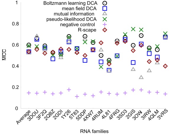
$\overline{MCC}$ of Boltzmann learning DCA, pseudolikelihood DCA, mean-field DCA, mutual information, and R-scape for 17 RNA families at the threshold obtained through cross-validation procedure. The recommended threshold 0.05 was used for R-scape. Families are labeled using the PDB code of the representative crystallographic structure. Average $\overline{MCC}$ is also reported. Alignments are performed with Infernal.

Influence of alignment method

We then used the two most accurate covariance methods (Boltzmann learning and pseudolikelihood DCA) to assess the influence of the alignment method. In particular, we considered the MSA methods implemented in ClustalW and Infernal packages. The average MCC over all RNA families when varying threshold S is systematically higher if sequences are aligned with Infernal rather than ClustalW (Fig. 4). We attribute this improvement in the quality of prediction performance to the use of consensus secondary structure in Infernal (Nawrocki and Eddy 2013). The discrepancy between the accuracies of contact prediction using two different alignment methods enlightens the necessity of efficient tools to improve covariance analysis input quality. Interestingly, the threshold score $\overline{S}$ maximizing the MCC is the same for the Boltzmann learning performed on the two different MSAs. This suggests the robustness of the adopted procedure to assess the optimal threshold score (Supplemental Eq. S14), again enlightening a greater consistency in its choice for the Boltzmann learning with respect to pseudolikelihood maximization framework. Given its better performance, the Infernal MSA method is used in the rest of the main text.

FIGURE 4.

Geometric-average MCC as a function of threshold scores S for Boltzmann learning and pseudolikelihood DCA. MSAs are performed with ClustalW and Infernal, as indicated. The sharp decrease after some method-dependent value of S is due to the fact that when the threshold is too large the number of correctly predicted contacts in at least one of the 17 investigated systems drops to zero.

Precision and sensitivity

In order to better quantify the capability of the investigated methods to provide useful information about contacts, we independently monitor sensitivity and precision for each RNA family at cross-validation thresholds. The average sensitivity values are around 0.3–0.4, indicating that approximately one third of the contacts present in the native structure can be predicted with these procedures (Supplemental Information, Fig. 1). Qualitatively, it appears that correctly predicted contacts are scattered along the sequences. The average precision instead ranges between 0.7 and 0.9, indicating that the number of falsely predicted contacts is rather small (Supplemental Information, Fig. 2). The Boltzmann learning and pseudolikelihood DCA report higher sensitivity and precision than the other methods. R-scape presents a higher sensitivity when compared with mutual information and a similar precision. We notice that R-scape results reported here are obtained using the recommended threshold (E-value <0.05). Results obtained choosing the E-value that maximizes the MCC are reported in Supplemental Information, Tables 9, 10. In order to assess the capability of these methods to probe RNA tertiary structure we also report the sensitivity value restricted to secondary contacts, obtained considering only base pairs contained in stems, and the number of true positive tertiary contacts, with results similar to those reported above (Supplemental Information, Figs. 3, 4). A contact is thus here considered as tertiary irrespectively of which edges are shared between nucleobases, and might even be an isolated WC pair. In general, DCA is able to identify not only cWW (Leontis and Westhof 2001) pairs, where covariance is mostly associated to canonical pairs (GC, AU, and GU), but also a number of noncanonical pairs (see Supplemental Information, Table 6). When looking at the absolute number of incorrect predictions the Boltzmann learning DCA provides the smallest average number (Supplemental Information, Fig. 5). In particular, pseudolikelihood DCA reports a very large number of false positives for a few systems. Also in this case, this is a consequence of the poor transferability of the cutoff for contact prediction in pseudolikelihood DCA. A more careful eye on incorrect predictions reveals that ≈50% of false positives predicted by all DCA methods are actually stacking interactions not included in the true-positive list since we only considered base-pairings in reference native structures (Supplemental Information, Table 7). In addition, couplings in consecutive nucleotides might be affected by a bias in the dinucleotide distribution.

Typical contact predictions

It is instructive to visualize which specific contacts are correctly predicted and which ones are not for individual systems. We first discuss the predictions on the systems where Boltzmann learning and pseudolikelihood DCA result in the highest MCC (glycine riboswitch, PDB 3OWI, and SAM riboswitch, PDB 2GIS, respectively). In the glycine riboswitch, Figure 5, we see that the two methods give comparable results. All the four native stems are predicted, although pseudolikelihood DCA predicts a slightly larger number of correct pairs. Also a non-stem WC contact is identified. In the SAM riboswitch, Figure 6, we see that the pseudolikelihood DCA predicts a significantly larger number of correct contacts. Notably, both methods are capable to identify contacts in a pseudoknotted helix between residues 25–28 and residues 68–65. These examples show that in the best cases these methods allow full helices to be identified accompanied by a small number of critical tertiary contacts. It is also useful to consider the cases resulting in the lowest MCC (SAM-I/IV riboswitch, PDB 4L81, for Boltzmann learning and NiCo riboswitch, PDB 4RUM, for pseudolikelihood DCA). In the SAM-I/IV riboswitch the two methods give comparable results, and only a limited number of secondary contacts are correctly predicted (Fig. 7). The stem between position 10 and position 20 shows a number of false positives. In this case, a helix with a register shifted by one nucleotide is suggested by the both DCA predictions. In more detail, we do not expect the alternative register to have a significant population in solution, since it would be capped by a AGAC tetraloop, whereas the reference crystal structure displays a common GAGA tetraloop. We interpret both sets of false positives as errors in the MSA. Indeed, especially with sequences consisting of consecutive identical nucleotides, one cannot assume the alignment procedure to correctly place gaps in the MSA. As a consequence, the reference structure for which the PDB is available might be misaligned with the majority of the homologous sequences in the MSA, resulting in predicted contacts shifted by one position upstream or downstream. Remarkably, many WC pairs close to the binding site of the riboswitch are predicted (G10/C21, G22/U50, and G23/C49; ligand directly interacts with nucleotides C7, A25, and U47). In the NiCo riboswitch, Figure 8, pseudolikelihood DCA only predicts six correct helical contacts, whereas Boltzmann learning DCA is capable to predict a number of contacts in the helices, even though resulting in several false positives. Figures 5–8 also report predictions done with R-scape.

FIGURE 5.

Glycine riboswitch (PDB code 3OWI) most accurate Boltzmann learning prediction (A) and respective pseudolikelihood prediction (B). Correctly predicted contacts in secondary structure are shown in dark gray. Correctly predicted tertiary contacts are shown in light gray. We notice that the G12/C28 pair is here labeled as tertiary since it corresponds to an isolated Watson–Crick pair in the reference structure. Prediction with R-scape is shown in C.

FIGURE 6.

SAM riboswitch (PDB code 2GIS), best accurate pseudolikelihood prediction (A), and respective Boltzmann learning prediction (B). Correctly predicted contacts in secondary structure are shown in dark gray. Correctly predicted tertiary contacts are shown in light gray. False positives are shown with dashed lines. Prediction with R-scape is shown in C.

FIGURE 7.

SAM-I/IV riboswitch (PDB code 4L81), least accurate Boltzmann learning prediction (A), and respective pseudolikelihood prediction (B). Correctly predicted contacts in secondary structure are shown in dark gray. Correctly predicted tertiary contacts are shown in light gray. False positives are shown with dashed lines. Prediction with R-scape is shown in C.

FIGURE 8.

NiCo riboswitch (PDB code 4RUM), least accurate pseudolikelihood prediction (A), and respective Boltzmann learning prediction (B). Correctly predicted contacts in secondary structure are shown in dark gray. Correctly predicted tertiary contacts are shown in light gray. False positives are shown with dashed lines. Prediction with R-scape is shown in C.

Validation on nonriboswitch systems

We further validated the whole procedure by considering 4 additional families including ribosomial RNA subunits, transfer RNA (tRNA), and a purely eukaryotic spliceosomal RNA. All the parameters of the Boltzmann learning simulations were chosen identical to those used for the riboswitch families. The threshold used to convert scores into predictions was taken as 1.06, which is the one that maximizes the MCC on the 17 riboswitch families. Results are reported in Supplemental Information, Table 12 and are slightly worse than those obtained for riboswitch families, with the exception of tRNA.

DISCUSSION

We here report a systematic assessment of RNA contact prediction based on aligned homologous sequences using mutual information analysis, R-scape, and DCA. When compared to previous works (De Leonardis et al. 2015; Weinreb et al. 2016; Wang et al. 2017), our analysis focuses on the DCA calculation and does not convert the resulting couplings into a structural model. The capability of various DCA-based methods to reproduce empirical frequencies from the MSA is evaluated. Native contacts in a set of reference structures are carefully annotated and compared with the predicted ones, in order to quantify the fraction of correctly predicted contacts (precision) and the fraction of predicted native contacts (sensitivity). In particular, since coevolution in RNA is expected to be related to isostericity (Leontis et al. 2002; Stombaugh et al. 2009), we only considered base-pairing and excluded other base-backbone or backbone-backbone contacts.

Our results show that ∼40% of the total native contacts can be predicted by this procedure. A large fraction of the predicted contacts are secondary structure contacts or pseudoknotted helices. However, in most of the analyzed structures, at least one tertiary contact is correctly predicted. In addition, the number of false positives is very small (≈10% of the predicted contacts). In many cases, false positives are just labeled so by our decision to exclude stacking interactions from the true contacts. In other cases, false positives are a consequence of an erroneous alignment of some of the sequences. Some false positives are genuinely caused by numerical noises or by the assumptions behind the Potts model. We notice that in principle the detrimental effect of false positives on the accuracy of structure prediction might be mitigated by using approaches where contacts that are not compatible with the predicted structure are discarded iteratively (Weinreb et al. 2016). As a general consideration, it must be kept in mind that strong couplings as predicted by DCA are a signature of coevolutionary pressure but not necessarily of spatial proximity. For instance, functionally related elements that are far from each other in space might exhibit coevolution. Relationships of this kind could in principle decrease the precision of the method in predicting contacts. In principle, highly conserved residues carry a limited amount of information and could thus reduce the sensitivity of the method, although in practice we never observed a very high conservation in the analyzed bacterial sequences. Eukariotic sequences might be more sensible to this issue, as it can be seen by the lower performance of the method when applied to spliceosomal RNA.

Importantly, we developed a rigorous manner to establish a threshold for contact prediction. In particular, once a figure of merit capable to take into account both the method precision and sensitivity has been defined, an optimal threshold can be found on a specific training set. We here used the Mathews correlation coefficient, that corresponds to the interaction network fidelity (Parisien et al. 2009) widely used in the RNA structure-prediction community (Miao et al. 2017). The resulting thresholds are different depending on the used method (mutual information vs. the tested DCA methods), but are transferable across different RNA families as illustrated by our cross-validation analysis.

It is important to observe that RNA molecules often display dynamics (i.e., coexistence of multiple structures) related to function, and that perhaps riboswitches are the paradigmatic example where multiple structures are required for function. For instance, some of the false positives might correspond to true contacts in an alternative, biologically functional structure (e.g., on and off state of the riboswitch). In addition, the alignment procedure itself might be more difficult or even not well defined in highly dynamic systems such as riboswitches. This fact might affect the results of the comparison reported here. Nevertheless, we believe that high resolution X-ray structures still represent the best proxy for the correct solution structure and as such they should be used for a critical assessment. Without having an experimentally determined ensemble, it appears difficult to assume that the observed false positives are, by chance, important contacts in alternative structures.

A crucial finding is that the here introduced stochastic solution of the inverse problem (Boltzmann learning) is feasible on these systems and outperforms the other DCA approaches. The resulting Potts models were shown to reproduce correctly the empirical frequencies from the MSA. Whereas the fact that the mean-field approach provides an approximate solution is well-known (Nguyen et al. 2017; Cocco et al. 2018), no such comparison has been reported on RNA DCA yet. Importantly, the few parameters required for the Boltzmann learning procedure can be tuned by monitoring the capability of the method to reproduce the empirical frequencies. The only parameter that is adjusted based on known structures is the threshold for contact prediction, that is here chosen with a cross-validation analysis. In addition, we show that, although it is supposed to be capable to infer correct couplings at least in the limit of a large number of sequences, also the pseudolikelihood approximation is not capable to reproduce the correct frequencies with the employed data sets. This fact was recently observed for protein systems (Figliuzzi et al. 2018), where it was also observed that in spite of this disagreement the contact predictions obtained with the pseudolikelihood approximation are of quality similar to those obtained with Boltzmann learning DCA.

The overall improvement in the accuracy of the predictions, as measured by the MCC, when passing from state-of-the-art pseudolikelihood DCA to Boltzmann learning DCA is due to the smaller number of false positives and is comparable to the one observed when passing from mutual information to mean-field DCA. Although the impact of this improvement should be assessed in a real 3D structure prediction test, we notice that the difference between mutual information and mean-field DCA was shown to significantly improve the quality of 3D structure prediction in De Leonardis et al. (2015). It is worth saying that the extra cost of the Boltzmann learning procedure is significant if one wants to characterize a large number of families. The required times for all the tested covariance methods scale roughly as the number of nucleotides squared and are listed in Table 1 for the largest and smallest molecules in the data set. If we also include the cost of a later 3D structure prediction and refinement, we consider the extra cost of Boltzmann learning to be absolutely worth. We believe that the fast Boltzmann learning procedure introduced here based on a stochastic gradient descent could be fruitfully used in protein systems as well. We also notice that the stochastic procedure used here is closely related to similar techniques used in the molecular dynamics community in order to enforce preassigned distributions in the generation of molecular structures (Valsson and Parrinello 2014; White and Voth 2014; Cesari et al. 2016, 2018). We chose here to use the simplest possible optimization algorithm, but more advanced procedures might make the Boltzmann learning approach even faster.

TABLE 1.

Computational time for the smallest and largest system investigated

We also tested the state-of-the-art pseudolikelihood maximization approach, which is faster than the Boltzmann learning approach but, on the tested data set, provides results of slightly inferior quality. Interestingly, the relatively good contact predictions obtained using pseudolikelihood DCA are not paralleled by correct frequencies in the reconstructed Potts model. Similar results were obtained decreasing the regularization term usually employed in pseudolikelihood DCA. This effect is likely due to the finite number of available sequences. A more important practical issue is that the optimal threshold used for contact predictions resulted less transferable across different families in pseudolikelihood DCA when compared with Boltzmann learning DCA. This suggests that choosing a cutoff that can single out true contacts might be more difficult in this method.

The impact on contact prediction of other sometime overlooked choices (reweighting and APC correction) has also been assessed. Our results show that these choices lead to negligible or minor improvements to all the methods.

Finally, we show that the alignment procedure used to prepare the MSA has a significant impact on the accuracy of the prediction. In particular, the Infernal algorithm, that is based on a previous prediction of the secondary structure, performs significantly better than the ClustalW algorithm. Whereas this effect is somewhat expected, we are not aware of similar assessments done on DCA methods. Interestingly, the effect of changing the alignment method is larger than the effect of optimally choosing all the other parameters, including the choice of using DCA rather than R-scape or the method used to infer DCA couplings. This suggests that the quality of the alignment is the issue that should be mostly addressed in future works in order to improve structure prediction based on coevolutionary information. We observe that the couplings obtained with the present approach might be used to further refine the multiple sequence alignments.

In conclusion, the direct-coupling analysis method was assessed on a number of RNA families. We found that, in spite of the intrinsic approximations, this procedure is able to reliably predict a number of contacts in RNA molecules with known three-dimensional structure. Among the tested methods, the Boltzmann learning approach is the one that allows to simultaneously maximize accuracy and precision. In perspective, we foresee the possibility to explicitly use information about the isosteric RNA families (Leontis et al. 2002; Stombaugh et al. 2009) or include three-body terms (Schmidt and Hamacher 2017) in order to further improve the accuracy of the predictions. Ultimately, we suggest the direct-coupling analysis performed through the Boltzmann learning as the best available tool to enhance RNA structure prediction for systems of up to a few hundred nucleotides, taking advantage of only homologous sequences information.

MATERIALS AND METHODS

Two multiple sequence alignment methods were tested, namely ClustalW (Thompson et al. 1994) and Infernal (Nawrocki and Eddy 2013). Empirical frequencies F_i (σ) and F_ij (σ, τ) were computed as discussed in Supplemental Information. In order to reduce the effect of possible sampling biases in the MSA we adopt the reweighting scheme as in (De Leonardis et al. 2015) with sequences similarity threshold 0.9. However, we did not find significant difference in test cases where the reweighting scheme was omitted (Supplemental Information, Table 5).

The idea of DCA is to construct a probability distribution in a parametric form so that the frequencies of nucleotides and co-occurence of nucleotides corresponding to the model, f_i (σ) and f_ij (σ, τ) coincide with the frequencies observed in the MSA, F_i (σ) and F_ij (σ, τ) (see Supplemental Methods). The distribution depends parametrically on a coupling matrix J that only contains direct interactions and is free of indirect correlations, hence the name direct couplings. In the following, we discuss the technical details associated to the Boltzmann learning procedure introduced here. For a more general introduction to DCA and to the other methods to perform DCA (mean field and pseudolikelihood) see Supplemental Methods.

Maximum likelihood and Boltzmann learning

Given a set of independent equilibrium configurations ${\left\{{\sigma }^b\right\}}_{b=1}^B$ of the model such that $P(\sigma )=\prod _{b=1}^{B}P\left({\sigma }^b\right)$, a statistical approach to infer parameters {h,J} is to let them maximize the likelihood, that is, the probability of generating the data set for a given set of parameters (Ekeberg et al. 2013). This can be equivalently done minimizing the negative log likelihood divided by the effective number of sequences:

$$l=-\frac{1}{B}\sum _{b=1}^B\log P\left({\sigma }^b\right).$$

Minimizing l with respect to local fields h_i gives

$$\begin{array}{rl}\frac{\mathrm{\partial }l}{\mathrm{\partial }{h}_i\left(\sigma \right)}=& -\frac{1}{B}\sum _{b=1}^B\left(\frac{\mathrm{\partial }\log Z}{\mathrm{\partial }{h}_i\left(\sigma \right)}-\delta ({\sigma }_i^b,\sigma )\right)\\ =& \frac{1}{B}\sum _{b=1}^B\left(f_i\right(\sigma )-\delta ({\sigma }_i^b,\sigma \left)\right)\\ =& f_i\left(\sigma \right)-F_i\left(\sigma \right)=0.\end{array}$$

Similarly, minimizing l with respect to the couplings gives

$$\frac{\mathrm{\partial }l}{\mathrm{\partial }{J}_{ij}(\sigma ,\tau )}=f_{ij}(\sigma ,\tau )-F_{ij}(\sigma ,\tau )=0.$$

These equations show that the model with the maximum likelihood to reproduce the sequences observed in the MSA is the one with frequencies identical to those observed in the MSA.

A possible strategy to minimize l is gradient descent, that is an iterative algorithm in which parameters are adjusted by forcing them to follow the opposite direction of the function gradient (Ackley et al. 1987; Sutto et al. 2015; Barrat-Charlaix et al. 2016; Haldane et al. 2016; Figliuzzi et al. 2018). The value of the parameters θ at iteration k + 1 can be obtained from the value of θ at the iteration k as

$${\theta }_{t+1}={\theta }_t-{\eta }_t{\mathrm{\nabla }}_{\theta }l\left(\theta \right)={\theta }_t-{\eta }_t\left(f\right(\theta )-F),$$

where η_t is the learning rate and t is the fictitious time, corresponding to the iteration number. Calculation of the gradient requires evaluation of an average over all the possible sequences. This average can be computed with a Metropolis–Hastings algorithm in sequence space, but might be very expensive due to the large size of the sequence space. In addition, the average should be recomputed at every iteration. We here propose to use the instantaneous value of δ(σ_i, σ), where σ_i is the identity of the nucleotide at position i in the simulated sequence, as an unbiased estimator of f_i (σ) in order to update the parameters more frequently, resulting in a stochastic gradient descent procedure that forces the system to sample the posterior distribution. The procedure can be easily parallelized, so that at each iteration the new set θ is an average of the updated parameters over all processes. We here used 20 simultaneous simulations initialized with 20 random sequences chosen in the MSA. Once parameters are stably fluctuating around a given value, their optimal value can be estimated by taking a time average of θ over a suitable time window (Cesari et al. 2018). At that point, a new simulation could be performed using the time-averaged parameters. Such a simulation can be used to rigorously validate the obtained parameters.

We here choose a learning rate η_t in the class search then converge (Darken and Moody 1990):

$${\eta }_t=\frac{\alpha }{1+{\displaystyle \frac{t}{{\tau }_S}}}.$$

This function is close to α for small t (“search phase”). For t ≫ τ_S the function decreases as 1/t (“converge phase”). Since it is based on Boltzmann sampling of the sequence space, we refer to this procedure as Boltzmann learning. The exact algorithm is described in the Supplemental Information and the employed C code is available at https://github.com/bussilab/bl-dca. We notice that in the algorithm implemented here, at variance with others proposed before (Sutto et al. 2015; Figliuzzi et al. 2018), the Lagrangian multipliers are evolved every few Monte Carlo iterations using istantaneous values rather than averages obtained from converged trajectories. In Figliuzzi et al. (2018) a change of variables of the model parameters was proposed to make the minimization easier. This idea might be beneficial also in our algorithm.

Validation of frequencies and predicted contacts

The capability of the tested DCA methods to reproduce the empirical frequencies was evaluated as discussed in Supplemental Methods. All the predicted contacts were validated against available crystallographic structures by computing the Matthews correlation coefficient (MCC) as discussed in Supplemental Methods. Particularly critical is the choice of the threshold used to identify predicted contacts, that is done using a cross-validation procedure where all the systems except one are used for training and the performance is evaluated only in the left out system (see Supplemental Methods). For R-scape, we used the recommended threshold $\overline{S}=0.05$.

SUPPLEMENTAL MATERIAL

Supplemental material is available for this article.

REFERENCES

- Ackley DH, Hinton GE, Sejnowski TJ. 1987. A learning algorithm for Boltzmann machines. In Readings in computer vision (ed. Fischler MA, Firschein O), pp. 522–533. Elsevier, Amsterdam. [Google Scholar]
- Arnold BC, Strauss D. 1991. Pseudolikelihood estimation: some examples. Sankhyā Ind J Stat Ser B 53: 233–243. [Google Scholar]
- Barrat-Charlaix P, Figliuzzi M, Weigt M. 2016. Improving landscape inference by integrating heterogeneous data in the inverse Ising problem. Sci Rep 6: 37812 10.1038/srep37812 [DOI] [PMC free article] [PubMed] [Google Scholar]
- Cesari A, Gil-Ley A, Bussi G. 2016. Combining simulations and solution experiments as a paradigm for RNA force field refinement. J Chem Theory Comput 12: 6192–6200. 10.1021/acs.jctc.6b00944 [DOI] [PubMed] [Google Scholar]
- Cesari A, Reißer S, Bussi G. 2018. Using the maximum entropy principle to combine simulations and solution experiments. Computation 6: 15 10.3390/computation6010015 [DOI] [Google Scholar]
- Cocco S, Feinauer C, Figliuzzi M, Monasson R, Weigt M. 2018. Inverse statistical physics of protein sequences: a key issues review. Rep Prog Phys 81: 032601 10.1088/1361-6633/aa9965 [DOI] [PubMed] [Google Scholar]
- Costa M, Michel F. 1997. Rules for RNA recognition of GNRA tetraloops deduced by in vitro selection: comparison with in vivo evolution. EMBO J 16: 3289–3302. 10.1093/emboj/16.11.3289 [DOI] [PMC free article] [PubMed] [Google Scholar]
- Darken C, Moody J. 1990. Note on learning rate schedules for stochastic optimization. In Proceedings of the 1990 conference on advances in neural information processing systems 3 NIPS-3, pp. 832–838. Morgan Kaufmann Publishers Inc., San Francisco. [Google Scholar]
- De Leonardis E, Lutz B, Ratz S, Cocco S, Monasson R, Schug A, Weigt M. 2015. Direct-coupling analysis of nucleotide coevolution facilitates RNA secondary and tertiary structure prediction. Nucleic Acids Res 43: 10444–10455. 10.1093/nar/gkv932 [DOI] [PMC free article] [PubMed] [Google Scholar]
- Doherty EA, Doudna JA. 2000. Ribozyme structures and mechanisms. Annu Rev Biochem 69: 597–615. 10.1146/annurev.biochem.69.1.597 [DOI] [PubMed] [Google Scholar]
- Dutheil JY, Jossinet F, Westhof E. 2010. Base pairing constraints drive structural epistasis in ribosomal RNA sequences. Mol Biol Evol 27: 1868–1876. 10.1093/molbev/msq069 [DOI] [PubMed] [Google Scholar]
- Eddy SR, Durbin R. 1994. RNA sequence analysis using covariance models. Nucleic Acids Res 22: 2079–2088. 10.1093/nar/22.11.2079 [DOI] [PMC free article] [PubMed] [Google Scholar]
- Ekeberg M, Lövkvist C, Lan Y, Weigt M, Aurell E. 2013. Improved contact prediction in proteins: using pseudolikelihoods to infer Potts models. Phys Rev E 87: 012707 10.1103/PhysRevE.87.012707 [DOI] [PubMed] [Google Scholar]
- Figliuzzi M, Barrat-Charlaix P, Weigt M. 2018. How pairwise coevolutionary models capture the collective residue variability in proteins? Mol Biol Evol 35: 1018–1027. 10.1093/molbev/msy007 [DOI] [PubMed] [Google Scholar]
- Haldane A, Flynn WF, He P, Vijayan R, Levy RM. 2016. Structural propensities of kinase family proteins from a Potts model of residue co-variation. Protein Sci 25: 1378–1384. 10.1002/pro.2954 [DOI] [PMC free article] [PubMed] [Google Scholar]
- Hon CC, Ramilowski JA, Harshbarger J, Bertin N, Rackham OJ, Gough J, Denisenko E, Schmeier S, Poulsen TM, Severin J, et al. 2017. An atlas of human long non-coding RNAs with accurate 5′ ends. Nature 543: 199 10.1038/nature21374 [DOI] [PMC free article] [PubMed] [Google Scholar]
- Jones DT, Buchan DW, Cozzetto D, Pontil M. 2011. PSICOV: precise structural contact prediction using sparse inverse covariance estimation on large multiple sequence alignments. Bioinformatics 28: 184–190. 10.1093/bioinformatics/btr638 [DOI] [PubMed] [Google Scholar]
- Leontis NB, Westhof E. 2001. Geometric nomenclature and classification of RNA base pairs. RNA 7: 499–512. 10.1017/S1355838201002515 [DOI] [PMC free article] [PubMed] [Google Scholar]
- Leontis NB, Stombaugh J, Westhof E. 2002. The non-Watson–Crick base pairs and their associated isostericity matrices. Nucleic Acids Res 30: 3497–3531. 10.1093/nar/gkf481 [DOI] [PMC free article] [PubMed] [Google Scholar]
- Lorenz R, Bernhart SH, Höner Zu Siederdissen C, Tafer H, Flamm C, Stadler PF, Hofacker IL. 2011. ViennaRNA package 2.0. Algorithms Mol Biol 6: 26 10.1186/1748-7188-6-26 [DOI] [PMC free article] [PubMed] [Google Scholar]
- Marks DS, Colwell LJ, Sheridan R, Hopf TA, Pagnani A, Zecchina R, Sander C. 2011. Protein 3D structure computed from evolutionary sequence variation. PLoS ONE 6: e28766 10.1371/journal.pone.0028766 [DOI] [PMC free article] [PubMed] [Google Scholar]
- Mathews DH, Disney MD, Childs JL, Schroeder SJ, Zuker M, Turner DH. 2004. Incorporating chemical modification constraints into a dynamic programming algorithm for prediction of RNA secondary structure. Proc Natl Acad Sci 101: 7287–7292. 10.1073/pnas.0401799101 [DOI] [PMC free article] [PubMed] [Google Scholar]
- Mathews DH, Turner DH, Watson RM. 2016. RNA secondary structure prediction. Curr Protoc Nucleic Acid Chem 67: 11–12. 10.1002/cpnc.19 [DOI] [PubMed] [Google Scholar]
- Miao Z, Adamiak RW, Antczak M, Batey RT, Becka AJ, Biesiada M, Boniecki MJ, Bujnicki JM, Chen SJ, Cheng CY, et al. 2017. RNA-puzzles round III: 3D RNA structure prediction of five riboswitches and one ribozyme. RNA 23: 655–672. 10.1261/rna.060368.116 [DOI] [PMC free article] [PubMed] [Google Scholar]
- Michel F, Westhof E. 1990. Modelling of the three-dimensional architecture of group I catalytic introns based on comparative sequence analysis. J Mol Biol 216: 585–610. 10.1016/0022-2836(90)90386-Z [DOI] [PubMed] [Google Scholar]
- Morcos F, Pagnani A, Lunt B, Bertolino A, Marks DS, Sander C, Zecchina R, Onuchic JN, Hwa T, Weigt M. 2011. Direct-coupling analysis of residue coevolution captures native contacts across many protein families. Proc Natl Acad Sci 108: E1293–E1301. 10.1073/pnas.1111471108 [DOI] [PMC free article] [PubMed] [Google Scholar]
- Morris KV, Mattick JS. 2014. The rise of regulatory RNA. Nat Rev Genet 15: 423 10.1038/nrg3722 [DOI] [PMC free article] [PubMed] [Google Scholar]
- Nawrocki EP, Eddy SR. 2013. Infernal 1.1: 100-fold faster RNA homology searches. Bioinformatics 29: 2933–2935. 10.1093/bioinformatics/btt509 [DOI] [PMC free article] [PubMed] [Google Scholar]
- Nawrocki EP, Burge SW, Bateman A, Daub J, Eberhardt RY, Eddy SR, Floden EW, Gardner PP, Jones TA, Tate J, et al. 2014. Rfam 12.0: updates to the RNA families database. Nucleic Acids Res 43: D130–D137. 10.1093/nar/gku1063 [DOI] [PMC free article] [PubMed] [Google Scholar]
- Nguyen HC, Zecchina R, Berg J. 2017. Inverse statistical problems: from the inverse Ising problem to data science. Adv Phys 66: 197–261. 10.1080/00018732.2017.1341604 [DOI] [Google Scholar]
- Pang PS, Jankowsky E, Wadley LM, Pyle AM. 2005. Prediction of functional tertiary interactions and intermolecular interfaces from primary sequence data. J Exp Zool B Mol Dev Evol 304: 50–63. 10.1002/jez.b.21024 [DOI] [PubMed] [Google Scholar]
- Parisien M, Cruz JA, Westhof É, Major F. 2009. New metrics for comparing and assessing discrepancies between RNA 3D structures and models. RNA 15: 1875–1885. 10.1261/rna.1700409 [DOI] [PMC free article] [PubMed] [Google Scholar]
- Ravikumar P, Wainwright MJ, Lafferty JD. 2010. High-dimensional Ising model selection using l1-regularized logistic regression. Ann Stat 38: 1287–1319. 10.1214/09-AOS691 [DOI] [Google Scholar]
- Rinnenthal J, Buck J, Ferner J, Wacker A, Fürtig B, Schwalbe H. 2011. Mapping the landscape of RNA dynamics with NMR spectroscopy. Acc Chem Res 44: 1292–1301. 10.1021/ar200137d [DOI] [PubMed] [Google Scholar]
- Rivas E, Clements J, Eddy SR. 2017. A statistical test for conserved RNA structure shows lack of evidence for structure in lncRNAs. Nat Methods 14: 45 10.1038/nmeth.4066 [DOI] [PMC free article] [PubMed] [Google Scholar]
- Schmidt M, Hamacher K. 2017. Three-body interactions improve contact prediction within direct-coupling analysis. Phys Rev E 96: 052405 10.1103/PhysRevE.96.052405 [DOI] [PubMed] [Google Scholar]
- Serganov A, Nudler E. 2013. A decade of riboswitches. Cell 152: 17–24. 10.1016/j.cell.2012.12.024 [DOI] [PMC free article] [PubMed] [Google Scholar]
- Smith MA, Gesell T, Stadler PF, Mattick JS. 2013. Widespread purifying selection on RNA structure in mammals. Nucleic Acids Res 41: 8220–8236. 10.1093/nar/gkt596 [DOI] [PMC free article] [PubMed] [Google Scholar]
- Šponer J, Bussi G, Krepl M, Banáš P, Bottaro S, Cunha RA, Gil-Ley A, Pinamonti G, Poblete S, Jurečka P, et al. 2018. RNA structural dynamics as captured by molecular simulations: a comprehensive overview. Chem Rev 118: 4177–4338. 10.1021/acs.chemrev.7b00427 [DOI] [PMC free article] [PubMed] [Google Scholar]
- Stombaugh J, Zirbel CL, Westhof E, Leontis NB. 2009. Frequency and isostericity of RNA base pairs. Nucleic Acids Res 37: 2294–2312. 10.1093/nar/gkp011 [DOI] [PMC free article] [PubMed] [Google Scholar]
- Sutto L, Marsili S, Valencia A, Gervasio FL. 2015. From residue coevolution to protein conformational ensembles and functional dynamics. Proc Natl Acad Sci 112: 13567–13572. 10.1073/pnas.1508584112 [DOI] [PMC free article] [PubMed] [Google Scholar]
- Thompson JD, Higgins DG, Gibson TJ. 1994. CLUSTAL W: improving the sensitivity of progressive multiple sequence alignment through sequence weighting, position-specific gap penalties and weight matrix choice. Nucleic Acids Res 22: 4673–4680. 10.1093/nar/22.22.4673 [DOI] [PMC free article] [PubMed] [Google Scholar]
- Valsson O, Parrinello M. 2014. Variational approach to enhanced sampling and free energy calculations. Phys Rev Lett 113: 090601 10.1103/PhysRevLett.113.090601 [DOI] [PubMed] [Google Scholar]
- Wang J, Mao K, Zhao Y, Zeng C, Xiang J, Zhang Y, Xiao Y. 2017. Optimization of RNA 3D structure prediction using evolutionary restraints of nucleotide–nucleotide interactions from direct coupling analysis. Nucleic Acids Res 45: 6299–6309. 10.1093/nar/gkx386 [DOI] [PMC free article] [PubMed] [Google Scholar]
- Weeks KM. 2010. Advances in RNA structure analysis by chemical probing. Curr Opin Struct Biol 20: 295–304. 10.1016/j.sbi.2010.04.001 [DOI] [PMC free article] [PubMed] [Google Scholar]
- Weinreb C, Riesselman AJ, Ingraham JB, Gross T, Sander C, Marks DS. 2016. 3D RNA and functional interactions from evolutionary couplings. Cell 165: 963–975. 10.1016/j.cell.2016.03.030 [DOI] [PMC free article] [PubMed] [Google Scholar]
- Westhof E. 2015. Twenty years of RNA crystallography. RNA 21: 486–487. 10.1261/rna.049726.115 [DOI] [PMC free article] [PubMed] [Google Scholar]
- White AD, Voth GA. 2014. Efficient and minimal method to bias molecular simulations with experimental data. J Chem Theory Comput 10: 3023–3030. 10.1021/ct500320c [DOI] [PubMed] [Google Scholar]
Associated Data
This section collects any data citations, data availability statements, or supplementary materials included in this article.