Current Experimental Methods for Characterizing Protein–Protein Interactions

Abstract

Protein molecules often interact with other partner protein molecules in order to execute their vital functions in living organisms. Characterization of protein–protein interactions thus plays a central role in understanding the molecular mechanism of relevant protein molecules, elucidating the cellular processes and pathways relevant to health or disease for drug discovery, and charting large‐scale interaction networks in systems biology research. A whole spectrum of methods, based on biophysical, biochemical, or genetic principles, have been developed to detect the time, space, and functional relevance of protein–protein interactions at various degrees of affinity and specificity. This article presents an overview of these experimental methods, outlining the principles, strengths and limitations, and recent developments of each type of method.

Protein–protein interactions play a central role in virtually all biological processes. A variety of experimental methods, based on either biophysical, biochemical, or genetic principles, have been developed for detecting protein–protein interactions. The results of these methods provide essential information for depicting the molecular mechanism of relevant protein molecules, the cellular pathways relevant to drug discovery, and large‐scale interaction networks in systems biology.

1.  Introduction

Proteins are vital components of living organisms as they are the main components of the physiological metabolic pathways of cells. The field of proteomics aims at studying the expression, structure, and function of all proteins on the whole genome level. It has been estimated that human genome consists of 19 000 genes coding for ∼500 000 proteins.1 Over 80 % of all proteins do not exist in isolation, but rather interact with one another to form stable or transient complexes.2 Protein–protein interactions (PPIs) thus play a central role in virtually all biological processes, such as metabolism, transport, structural organization, signal transduction, cell‐cycle control, immune recognition, and gene transcription.3 Completion of a genome sequencing project is normally accompanied with a vast growth of unannotated proteins. Identification of PPIs assists in functional assignment of novel proteins by situating them relative to other proteins in cellular pathways or functional classes,4 derives a better understanding of the biological relevance of protein functions, and provides key information from which to elucidate the functioning of a living cell under both physiological and pathological conditions. Moreover, investigation of PPIs on a large scale, that is, so‐called interactomes, is the foundation for systematic analysis of cellular networks. Cells can be envisioned as a complex web involving innumerable PPIs. Mapping PPI networks for model organisms and human to elucidate the organization of the proteome is one of the important goals for systems biology research, which paves the way to unravel the functional, logical and dynamical aspects of cellular systems.5

Notably, since aberrant PPIs contribute to the pathogenesis of numerous human diseases, PPIs are considered to be an emerging class of drug targets for therapeutic intervention. Target‐based drug discovery has slowly shifted from a protein‐centric view, largely focusing on some validated therapeutic targets such as G protein‐coupled receptors (GPCRs), nuclear hormone receptors, ion channels and enzymes, towards a more holistic, pathway‐centric view.6 Modulating PPIs implicated in cancer, virology, cardiovascular, or immunology, such as Bcl‐2/Bcl‐x_L–Bax/Bak,7 p53–MDM2,8 CCR5–HIV‐1 gp120,9 fibrinogen–GPIIb/IIIa,10 CD80–CD28,11 offers the opportunity to develop novel drugs for the treatment of the corresponding disease. In fact, about a dozen of PPI modulators have entered clinical trials or even successfully been developed into marketed drugs.12, 13, 14

Generally, PPIs can be classified into two main categories based on the contact interface: domain–domain and domain–motif interactions. Domain–domain interaction involves the binding of two globular domains that creates a large contact interface (∼2000 Ų), with relatively strong affinities in the low nanomolar or even picomolar range. For domain–motif interaction, a short linear motif (up to 20–30 amino acid residues) on a protein molecule binds to its interacting partner with affinities in the low‐ to mid‐micromolar range, forming a much smaller contact interface (∼300–500 Ų).15 A recent analysis estimated that the human proteome contains over 35 000 domains and 100 000 motifs.16 This estimation provides a rough idea of the size of the protein–protein “interactome ”.

A variety of experimental methods, based on either biophysical, biochemical, or genetic principles, have been developed to aid studies on PPIs. Each type of method has its own strengths and limitations in terms of sensitivity and specificity. Thus, they lay emphasis on different aspects of PPI analysis, for example, to identify binding partners of protein of interest, to generate structure details of protein complexes, to determine kinetic and thermodynamic constants of PPIs, to visualize and quantify PPIs in real time in living cells, and to map small interactomes referring to specific cellular pathways. Herein, we describe some widely applied experimental methods for characterizing PPIs, summarizing the principles, applications, pros/cons, and recent developments of each type of method.

2.  Biophysical Methods

A variety of biophysical methods can be used for the detection of PPIs, and the most prevalent are summarized in Table 1 and discussed in detail below.

Table 1.

Comparison of biophysical methods for the detection of protein–protein interactions (PPIs).

Method	Advantages	Disadvantages	Affinity range	Sample consumption
Fluorescence polarization (FP)	Automated high throughput; mix‐and‐read format; low cost	Relies on a comparatively large change in size upon binding; suffers from interference from autofluorescence, quenching and light scattering	nm to mm	Dozens of μL at nm concentration per data point
Surface plasmon resonance (SPR)	Label‐free; real‐time kinetic measurement	Surface immobilization can interfere with the binding event	sub‐nm to low mm	Several μg per sensor chip
Nuclear magnetic resonance (NMR)	High structural resolution	Internal protein labelling required; high sample consumption; long time to analyze obtained spectra	μm to mm	Several mg per data point
Circular dichroism (CD)	Label‐free; quick assay	Low structural resolution; low throughput	pm to μm	Dozens of ug per data point
Static and dynamic light scattering (SLS/DLS)	Label‐free; noninvasive	DLS requires an obvious difference in the hydro‐ dynamic radius of the unbound partners relative to the complex	pm to mm	Several μL at pm concentration per data point
Analytical ultra‐ centrifugation (AUC)[a]	Label‐free	Long duration for SE assay	nm to mm	Several hundred μL at nm to μm concentration per data point
Isothermal titration calorimetry (ITC)	Label‐free; provides thermo‐ dynamic parameters	Low throughput and sensitivity; long preparation time; buffer limitation	nm to sub‐mm	Several hundred μg per binding assay
Microscale thermo‐ phoresis (MST)	Fast measurement times; low sample consumption	Fluorescent labelling is required for typical MST	pm to mm	Several μL at nm concentration

[a] Two types of AUC experiments: sedimentation velocity (SV) and sedimentation equilibrium (SE).

This article is being made freely available through PubMed Central as part of the COVID-19 public health emergency response. It can be used for unrestricted research re-use and analysis in any form or by any means with acknowledgement of the original source, for the duration of the public health emergency.

2.1.  Fluorescence polarization (FP)

The theory of fluorescence polarization (FP) was first described in 1926,17 and it is based on the observation of the molecular movement of fluorophores in solution. When a fluorophore is excited by polarized light, it emits light with unequal intensities along different axes of polarization. The degree of polarization is inversely related to molecular rotation of the fluorophore, which is largely dependent on molecular mass. Typically, larger masses show slower rotation.18 With adequate experimental design, an FP assay can be used to measure binding and dissociation between two molecules if one of the binding molecules is relatively small and labeled with a fluorophore (Figure 1 A). Commonly used fluorophores for an FP assay include fluorescein, rhodamine, BODIPY (boron‐dipyrromethene), and Cy5 (cyanine‐5) dyes, or their derivatives. Complex formation leads to an increase in FP signal (in millipolarization units, mP), which can be measured by a microplate reader. A binding curve can be generated by plotting mP values against multiple concentrations of the labeled molecule. Then, the dissociation constant (K _d) between two binding molecules can be determined from the curve.

Figure 1.

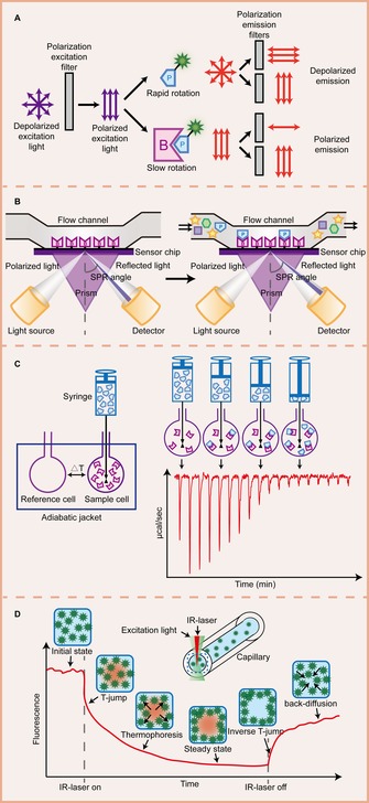
Illustration of some biophysical methods for PPI detection. A) Fluorescence polarization (FP). When a fluorescently labelled small molecule is excited by polarized light, it emits lights with a certain degree of polarization that is inversely proportional to the rotation rate of the fluorescent molecule. A small molecule rotates fast, so the emitted lights are depolarized. Its rotation is greatly decreased when it binds to a larger molecule, so the emitted light remains polarized. B) Surface plasmon resonance (SPR). In an SPR biosensor, an incident light beam hits a prism covered with a thin gold film at a certain angle, leading to the phenomenon of SPR. Perturbations at the gold surface on the sensor chip, such as the interaction between the bait immobilized on the surface and the prey flown over the surface, result in detectable SPR angle shifts. C) Isothermal titration calorimetry (ITC). An ITC instrument is composed of a reference cell and a sample cell, both of which are surrounded by an adiabatic jacket. During measurement, a protein molecule loaded in the syringe is titrated into the sample cell containing its binding partner, causing heat changes in the sample cell. This heat change can be quantified by the electric power required to maintain the isothermal condition between two cells. D) Microscale thermophoresis (MST). The sample solution containing fluorescent molecules inside a capillary is heated by a focused IR‐laser, which is coupled into the path of fluorescence excitation and emission. A series of processes, including initial state, T‐jump, thermophoresis, steady state, inverse T‐jump, and back‐diffusion of fluorescent molecules can be detected through the temperature gradient.

FP assays have been widely used in PPI studies, for example to estimate the binding between initiation factor 3 (IF3) and 30S ribosomal subunits,19 initiation factor 2 (IF2) and 30S ribosomal subunits,20 gene 2.5 protein and DNA polymerase of bacteriophage T7,21 and others. As PPIs are often governed by a small number of “binding epitopes”, for example, hot spots, utilizing short truncated motifs containing such epitopes mimics the interactions between two complete protein molecules and thus facilitates experimental measurements. Such an FP assay also provides an opportunity for the detection of inhibitors targeting the PPI.22 For instance, an FP competition assay has been developed to identify inhibitors targeting the MDM2–p53 peptide interaction,23 to screen small molecules that inhibit the ZipA–FtsZ peptide interaction,24 to screen natural product extracts that disrupt the binding of antiapoptotic Bcl‐2 family members to Bim BH3 peptides.25 The advantages of an FP assay are its low cost, simple mix‐and‐read format without wash steps, and the high‐throughput screening (HTS) capacity of the assay when carried out in a multiwell plate (96/384/1,536). However, like other fluorescence‐based assays, it also suffers from some drawbacks, such as interference from auto‐fluorescence, quenching, and light scattering.26

2.2.  Surface plasmon resonance (SPR)

Surface plasmon resonance (SPR) is a quantum electromagnetic phenomenon that occurs at a metal‐dielectric interface. When a photon of lights hits the metal surface (typically a gold film) at a certain angle of incidence, the light energy is transferred to collective excitations of free electrons, called surface plasmons, and generates electromagnetic waves that propagate along the interface. Resonant transfer of light energy to surface plasmons leads to a sharp attenuation in the reflected light. The angle of incidence at which minimum reflection occurs is defined as the SPR angle. A slight change near the interface (e.g., a change in refractive index in the vicinity of the metal surface) leads to a change in the SPR angle.27, 28 A biosensor system based on SPR has become one of the most popular sensing technology for measuring molecular interactions. In an SPR experiment, the bait protein is first immobilized onto the sensor chip, which is then perfused with buffer solution containing analytes. If interaction occurs, the accumulation of analytes on the sensor surface induces an increase in the refractive index at the sensor surface, and the SPR angle is shifted (Figure 1 B). During dissociation, the inverse effect is observed. The RU (termed response or resonance unit) is recorded to describe this signal change, where one RU is equivalent to a critical angle shift of 10⁻⁴ degree.29 Since the first commercial SPR‐based analytical instrument launched by Biacore AB in 1990, other competing SPR biosensor systems have been developed by manufacturers such as Affinity Sensors, IBIS Technologies, Texas Instruments, Aviv, and BioTul AG.30 As the interface between the sensor surface and the interacting proteins to be studied is a vital component of this surface‐sensitive sensor system, several robust and reproducible sensor chips from Biacore are commercially available, such as the CM5 chip (carboxymethylated dextran covalently attached to a gold surface) for immobilization via amine, thiol, aldehyde, or carboxyl groups of proteins, the NTA chip (carboxymethylated dextran pre‐immobilized with nitrilotriacetic acid) for immobilization of His‐tagged proteins, SA chip (carboxymethylated dextran pre‐immobilized with streptavidin) for immobilization of biotinylated proteins.31

SPR biosensor technology has various technical advantages, which has been proven useful for verifying PPIs.^[32–34] Small amounts of sample are needed (micro to sub‐micrograms) without labeling requirements. It is capable of characterizing binding reaction in real time, determining kinetic and thermodynamic constants of biomolecular interactions, and allowing the analysis of interactions with a wide range of molecular weights, affinities and binding rate. A potential limitation is its sensitivity to interfering effects such as nonspecific interaction between the sensor surface and analyte.35 Additionally, the requirement for immobilization might disturb the interactions under measurement. The SPR technique has traditionally been used in low‐throughput studies as standard SPR biosensor only contains three to four flow cells on a single sensor chip. Nowadays, SPR imaging (SPRI) is extended towards HTS. By utilizing protein array technology and a charge‐coupled device (CCD) camera to make images based on the intensity of reflected light, SPRI has been developed to simultaneously process hundreds or thousands of samples.28, 36 Furthermore, using the SPR technique coupled with mass spectrometry (MS) enables the discovery of novel PPIs.^[27, 37]

2.3.  Nuclear magnetic resonance (NMR)

Nuclear magnetic resonance (NMR) is a physical phenomenon whereby magnetically active nuclei in a strong magnetic field absorb electromagnetic radiation at distinct frequencies that are determined by the chemical environment of each nucleus.38 The most prominent applications of NMR spectroscopy are the characterization and determination of the structures of biological macromolecules in solution, including generating structural details of protein interactions at an atomic resolution. Various NMR parameters providing angular or distance data are primary sources of conformational information, including (1) chemical shift perturbation, which is the chemical shift (resonance frequency) change of a nucleus in the protein induced after addition of an interacting partner. In particular, heteronuclear single‐quantum coherence (HSQC) NMR experiments are widely used to delineate protein–protein interfaces;39, 40 (2) the nuclear Overhauser effect (NOE) is the NMR equivalent of fluorescence resonance energy transfer (FRET), discussed later in Section 3.1, referring to the transfer of nuclear spin polarization from one nuclear spin population to another via dipolar cross‐relaxation, the intensity of which is proportional to the inverse‐sixth power of the distance between two nuclei. Many precise NOE‐derived distance constraints between two proteins with tight interaction (K _d≤10 μm) can be used to determine the full 3D structure of the complex;41, 42 (3) paramagnetic relaxation enhancement (PRE), arising from magnetic dipolar interactions between the unpaired electron in a paramagnetic center and a nearby NMR‐active nucleus, provides long‐range distance information that can complement NOE restraints;43, 44 (4) residual dipolar couplings (RDCs), reporting on relative orientations among internuclei vectors irrespective of their distance separations, can provide orientation restraints for structural characterization of protein complexes.45, 46 Other NMR data includes cross‐saturation, pseudo‐contact shift, J coupling, and so on. A combination of these NMR‐derived restraints can help to obtain a more refined structure of a given PPI with a very wide range of dissociation constants (from 10⁻⁶ to 10⁻²  m).47

As the conventional application of NMR spectroscopy is often oriented to soluble proteins, solid‐state NMR spectroscopy has evolved to study membrane proteins involved in PPIs in liquid crystalline lipid bilayers as a more native‐like membrane mimetic environment.48 Another attractive progress in NMR technology is the in‐cell NMR spectroscopy, which allows the exploration of PPIs under physiological conditions in living cells.49

2.4.  Circular dichroism (CD)

Circular dichroism (CD) spectroscopy measures differences in absorption of left and right circularly polarized light that arise due to structural asymmetry, and it is often reported in units of ellipticity. A CD spectrum of a protein in the far‐UV region (190–250 nm) arises from the amide groups on the protein backbone and is sensitive to the secondary structure of the protein including alpha‐helix, beta‐sheet, and random coil structures. While a CD spectrum in the near‐UV (250–320 nm) region arises from aromatic amino acids and disulfide bonds, and is sensitive to certain aspects of the tertiary structure of the protein.50 Thus, changes in the CD spectrum can provide information about the changes in protein conformation.

Various methods have been used to analyze protein conformational changes accompanying PPIs by studying the CD spectra, such as CONTIN: a program that estimates the changes in secondary structure of the catalytic subunit of cAMP‐dependent protein kinase when bound by Kemptide,51 MLR: a program designed to elucidate the mechanism and structural requirements of the interaction of tropomodulin with tropomyosin,52 SELCON, CDNN, K2D, and so on.53

As CD spectroscopy is a quantitative technique and the change in CD upon binding is directly proportional to the amount of complex formed, the association or dissociation constant of the complex can also be determined by using CD by direct titration of one protein by another.52, 54 An enhanced version, termed synchrotron radiation circular dichroism (SRCD), extends the utility and applications of conventional CD by using a synchrotron ring instead of a xenon arc lamp as the light source. This version enables collection of data in the vacuum UV region (<190 nm), detection of spectra with improved signal‐to‐noise ratios, and measurements for PPIs involving either induced‐fit or rigid‐body mechanisms.55, 56 Besides information related to conformational changes, analysis of CD spectra obtained at different temperatures can provide thermodynamic parameters (such as binding constants) of interacting protein molecules.57

Generally, CD spectroscopy is a quick method that does not require large amounts of proteins or extensive data processing, and it can be conducted under varying conditions, including solvent, temperature, and pH. However, as a spectroscopic method for characterization of protein structures, CD gives less specific information than NMR spectroscopy.

2.5.  Static and dynamic light scattering (SLS/DLS)

Light scattering refers to a physical process involving the interaction of light with a small particle or molecule. When an incident photon encounters a molecule, it perturbs the electron orbits within the molecule and creates an induced dipole moment, which becomes a source of electromagnetic radiation with energy radiated in all directions. The evaluation of the scattered light with regard to its intensity and wavelength often yields valuable information about the scattering molecules, such as molar mass, binding affinity, and absolute stoichiometry of complex interactions. This makes light scattering a versatile tool for characterization of macromolecules and their interactions in solution.58 In contrast to most methods for characterization, light scattering is an absolute measurement without requiring outside calibration standards.

The most widely used light scattering techniques are static light scattering (SLS) and dynamic light scattering (DLS). In SLS, also known as classical light scattering or multiple angle light scattering, time‐averaged scattered light intensity is collected at multiple different angles, with weight average molar mass, size and shape of molecules, and second virial coefficient reflecting PPIs calculated from this data. In DLS, also known as quasi‐elastic light scattering, the fluctuations in the intensity of scattered light at a certain angle as the effect of the Brownian motion of the scattering molecules is detected, yielding information about translational diffusion coefficient and hydrodynamic radius of molecules.59 Combining a light scattering detection technique and a separation system, such as size‐exclusion chromatography, provides a good method for the semi‐quantitative characterization of PPIs with high sensitivity and high resolution in short run times.58, 60 As interaction studies should be performed under true equilibrium, a series of batch SLS or DLS measurements over varying compositions referred to as composition‐gradient SLS (CG‐SLS) or DLS (CG‐DLS) have been used to determine equilibrium properties including association stoichiometry and binding affinity of interacting macromolecules in solution.61, 62

2.6.  Analytical ultracentrifugation (AUC)

Analytical ultracentrifugation (AUC) is a classical method for detecting the concentration distribution of the macromolecule in solution in real‐time under centrifugal force, and providing first‐principle hydrodynamic and thermodynamic information about the size, shape, molar mass, association energy, association stoichiometry and thermodynamic nonideality of the molecules.63 Two types of AUC experiments exist, sedimentation velocity (SV) and sedimentation equilibrium (SE). An SV experiment is usually conducted at a very high rotor speed, leading to the depletion of macromolecules from the meniscus region at the air/solution interface and the formation of a concentration boundary that moves toward the bottom of the centrifuge cell as a function of time.64 It has been employed to determine the relative energetics of the homo‐ and hetero‐dimerization of BirA by using SEDFIT, SC‐ISOTHERM, and SEDANAL,65 and to reveal the significance of hydrolysable ATP in the complex formation between cpn60 and cpn10.66

In contrast, an SE experiment is conducted at lower rotor speeds, when the centrifugal and back‐diffusive forces come to thermodynamic equilibrium. It yields a steady‐state concentration distribution that is a function of buoyant solute mass, mass distribution, and mass action parameters for interacting systems, such as the equilibrium association constant or equivalent dissociation constant.67 SE has been applied to evaluate the K _d value for the CD2–CD48 interaction,68 and to study the stoichiometry and affinity of the SCF–Kit interaction.69 A variant of the SE technique called “tracer SE”, in which one of the solute components is labeled, facilitates the study of both self‐ and hetero‐associations over an unprecedentedly broad range of concentration with increased resolution.70 The disadvantages of SE include long duration for the completion of the experiment.

Generally speaking, AUC is a powerful method for studying macromolecules over a wide range of concentrations and in a wide variety of solvents. The results produced by this method are absolute and independent of standards for comparison as it relies on the principal property of mass and the fundamental law of gravitation.

2.7.  Calorimetric methods

Calorimetry relies on the fact that all chemical reactions are accompanied by an endothermic or exothermic change in energy. In PPIs, the change in conformation of interacting proteins from the free to the bound state produces a plethora of bond rearrangements, including hydrogen bonds, van der Waals interactions, and hydrophobic interactions formed or broken, which result in an overall change in the Gibbs energy of the system.71 Calorimetric methods can directly determine the thermodynamic parameters as a probe for an interaction by detecting the heat energy changes. Currently, two super‐sensitive calorimetric techniques with commercially available instruments, that is, isothermal titration calorimetry (ITC) and differential scanning calorimetry (DSC), are widely applied.

ITC directly quantifies the heat change in a reaction at constant temperature or heat capacity at multiple temperatures; it is easy to perform with commercially available high‐sensitivity instruments, such as MicroCal VP‐ITC and iTC200. In a typical ITC experiment, one interacting protein placed in the injection syringe is titrated in small aliquots into another in a sample cell, which is temperature controlled and coupled to a reference cell via a sensitive thermopile/thermocouple circuit. The heat either released (an exothermic reaction) or absorbed (an endothermic reaction) at equilibrium conditions over the course of titration can be measured directly with sufficient sensitivity (in the order of several hundred nanojoules)72 (Figure 1 C). ITC does not suffer from constraints of molecular size, shape or chemical constitution. Neither is there any need for immobilization or modification of proteins.73 However, extreme care must be taken in the use of a buffer in an ITC experiment, that is, both interacting proteins in the sample cell as well as the syringe should be dialyzed in an identical buffer to minimize the artifacts generated by mismatched buffer components.74 The main parameters extracted from ITC experiment include association constant (K _a), enthalpy change (ΔH), reaction stoichiometry (n), heat capacity change (ΔC _p), free energy change (ΔG) and entropy change (ΔS).75 These data help us better understand both the affinities and mechanisms of PPIs, for example, estimating the hydrophobic effect of a residue at protein–protein interface by calculating changes in solvent portion of the binding entropy,76 determining exact contributions to binding including solvation, protonation, and structural rearrangements,77 validating oligomeric state of a protein during binding events according to stoichiometry data.78

DSC measures the heat effects of temperature‐induced transitions of proteins in dilute solutions. Most modern DSC instruments, such as nano‐DSC from Calorimetry Science Corp., have two cells: a sample cell containing interacting proteins and a reference cell containing only solvent. By applying a controlled temperature program heating up to 100 °C or cooling down to 0 °C at a constant rate, the power required to maintain identical temperature between two cells is converted into molar heat capacity and recorded as a function of temperature.79, 80 From a DSC thermogram, the transition temperature (T _m), enthalpy change (ΔH) and heat capacity change (ΔC _p) can be obtained. As the thermal stability of proteins will be affected by complex formation, DSC experiments can be used to study PPIs by observing shifts in T _m values.81, 82, 83

2.8.  Microscale thermophoresis (MST)

Microscale thermophoresis (MST) emerged as a new powerful technique for quantitative analysis of PPIs in free solution, which has been applied widely in academia and industry. This technique detects the directed motion of molecules in a microscopic temperature gradient, an effect termed thermophoresis. This effect is highly sensitive to binding‐induced changes in various molecular properties, such as size, charge, conformation or hydration shell.84 In a typical MST experiment, one of the interacting proteins is fluorescently labeled. It is normally done by using N‐hydroxysuccinimide (NHS) dye to react with a primary amine group on the labeled protein, or a recombinant protein fused to a fluorescent protein such as green fluorescent protein (GFP). Alternatively, MST can be performed in a label‐free manner, in which the intrinsic UV‐fluorescent signal of the aromatic amino acid residues is detected. A MST instrument uses an infrared (IR) laser to heat a defined sample volume inside a capillary and produces a temperature gradient spanning 2–6 K. The thermophoretic movement of the fluorescent protein is measured by detecting the fluorescence emission of the heat spot within the sample before, during, and after the IR laser is switched on. Before heating, the initial fluorescence is recorded at a constant level. Once the IR laser is switched on, the increase of temperature leads to an abrupt decrease in fluorescence intensity, so called temperature jump (T‐jump). After that, the fluorescence decreases slowly (thermophoresis) until reaching a steady state. When the IR laser is switched off, the fluorescence recovery (inverse T‐jump and back‐diffusion) is observed85, 86, 87 (Figure 1 D). During this procedure, both T‐jump and the thermophoresis process can be affected by a binding event due to changes in size, charge or hydration shell. Hence, MST can be applied to determine dissociation constants of PPIs via titration, in which a constant concentration of fluorescent protein and varying concentrations of its nonfluorescent binding partner are applied.84, 88, 89

MST has several advantages over other in vitro biophysical methods, including easy setting, fast measurement (binding affinity is determined in 10 min), and low sample consumption (a few microliters at nanomolar concentrations). It allows quantitative measurement of high‐affinity interactions with dissociation constant in the picomolar range. In addition, it can be performed in any buffer or even in complex bioliquids like blood serum or cell lysate.87, 90

3.  Biochemical Methods

3.1.  Fluorescence and bioluminescence resonance energy transfer (FRET and BRET)

Fluorescence resonance energy transfer (FRET) refers to the nonradiative (dipole–dipole) energy transfer from a donor fluorophore (fused to the “bait”) upon excitation to an acceptor fluorophore (fused to the “prey”).91 In PPI studies, intermolecular FRET only occurs when the bait and the prey are engaged in complex formation that brings two fluorophores in very close proximity (1–10 nm) (Figure 2 A). Furthermore, a donor–acceptor FRET pair requires an overlap between the emission spectrum of the donor and the excitation spectrum of the acceptor to obtain efficient energy transfer. The widely used FRET pairs come from variants of GFP, for example, cyan fluorescent protein (CFP)–yellow fluorescent protein (YFP), blue fluorescent protein (BFP)–GFP,92 CyPet–Ypet,93 MiCy–mKO,94 cerulean fluorescent protein (CrFP)–YFP,95 and mVenus–mStrawberry.96 Such large fluorophore can also be replaced by a small, membrane‐permeable fluorescein derivative termed FlAsH, which targets to a short tetracysteine motif (e.g., CCPGCC) introduced to the protein sequence without disturbing the protein function.97

Figure 2.

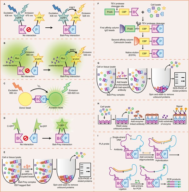
Illustration of some biochemical methods for PPI detection. A) Fluorescence resonance energy transfer (FRET) between a CFP‐fused bait and a YFP‐fused prey, where CFP and YFP act as the donor and the acceptor fluorophore, respectively. If the bait and the prey do not interact, excitation of CFP results in light emission (475 nm) by CFP only. When bait–prey interaction occurs, CFP and YFP are brought into proximity, leading to energy transfer from CFP to nearby YFP. Then, YFP emission can be detected at 528 nm. B) Bioluminescence resonance energy transfer (BRET) between a Rluc‐fused bait and a EYFP‐fused prey, where Rluc and EYFP act as the donor luciferase and the acceptor fluorophore, respectively. If bait and prey do not interact, only the blue‐emitting spectrum (480 nm) of RLuc can be detected. When bait–prey interaction occurs, bioluminescence energy generated by Rluc in the presence of its substrate (coelenterazine) is transferred to EYFP, which in turn generates light emission at 530 nm. C) AlphaScreen. Upon excitation at 680 nm, a photosensitizing agent on the donor bead converts ambient oxygen to singlet oxygen. When bait–prey interaction brings the donor and the acceptor bead into close proximity, energy is transferred from singlet oxygen to thioxene derivatives on the acceptor bead, resulting in light emission at 520–620 nm. D) Protein‐fragment complementation assay (PCA). Complementary C‐terminal and N‐terminal fragments of GFP are fused to the bait and the prey, respectively. If the bait and the prey do not interact, the fragments remain unstructured and lack functional activity. When the bait–prey interaction occurs, two fragments are brought together to form a full‐length GFP with the native structure and function. E) Pull‐down assay. In a GST pull‐down assay, the bait is expressed as a GST‐fused protein, and it is incubated with cell or tissue lysate containing the prey. The GST–bait–prey complex is captured by glutathione‐coupled beads and eluted for analysis by SDS‐PAGE. F) Tandem affinity purification (TAP). In this type of assay, the TAP tag (including CBP, a TEV cleavage site, and ProtA) is fused to the bait, and then the whole construction is introduced into the host cell. The TAP–bait–prey complex is isolated from cell lysate via affinity column containing IgG beads. After washing, TEV protease is added to release the CBP–bait–prey complex, which is then immobilized on calmodulin‐coated beads. After washing, the native complex is eluted by chelating calcium using EGTA. G) Co‐immunoprecipitation (Co‐IP). The bait–prey complex in cell or tissue lysate is captured by beads functionalized with a bait‐specific antibody, and then co‐precipitated, washed, eluted, and analyzed by SDS‐PAGE. H) ELISA. In the case of direct ELISA, the bait is immobilized on a microwell plate, and then cell lysate containing the prey is applied to the wells. After incubation and washing away unbound proteins, the bait–prey complex is detected by an HRP‐conjugated antibody against the prey. Finally, a substance of the HRP enzyme is added, which in turn produces detectable fluorescence‐ or absorbance‐based signal via the enzymatic reaction. I) Proximity ligation assay (PLA). The bait and prey are recognized by their respective PLA probes consisting of antibodies and single‐stranded DNA oligonucleotides, where the free oligonucleotide ends are brought into proximity. An oligonucleotide connecter is added to hybridize to the complementary oligonucleotides on the PLA probes. A ligase seals the nick between two PLA probes and forms a new DNA strand that can be amplified by PCR.

With the development of optimized FRET pairs, FRET has been applied to in vitro binding assay for screening of PPI inhibitors.98, 99 Combined with microscopy imaging technologies, it can also be used to visualize and quantify PPIs in real time in living cells, with high spatiotemporal resolution.100, 101, 102 As FRET microscopy relies on the ability to collect fluorescent signals from protein interactions, it suffers from some drawbacks, including auto‐fluorescence, detector noise, optical noise, photobleaching, and spectral bleedthrough signals (partial overlap of donor and acceptor emission wavelengths).103 Therefore, several methods have been used to correct for these problems and calculate FRET efficiency, each with its own strengths and weaknesses,104 including sensitized emission,105, 106 acceptor photobleaching,107, 108, 109 fluorescence life‐time imaging microscopy (FLIM),110, 111, 112 spectral imaging,113, 114 and fluorescence polarization imaging.115, 116 FRET experiments can also be performed using a flow cytometer. This type of experiment allows the analysis of a large number of cells in a short time, producing statistically more robust results than the microscope technique. However, it cannot be used to analyze intracellular structures.108, 117, 118 Applicability of FRET with a laser scanning cytometer (LSC) combines attributes of both microscopy and flow cytometry, and yields information on a pixel‐by‐pixel and cell‐by‐cell basis.119

Time‐resolved FRET (TR‐FRET) is a special form of FRET in which long‐life emission fluorophores (lanthanides such as europium and terbium) are used as donors. Commonly used donor–accepter pairs includes europium chelate or cyptate–allophycocyanin,120, 121 europium chelate–Cy5,122 europium chelate–Dy647,123 terbium cryptate–d2,124 and terbium–AF488.125 As carriers of lanthanides, chelate and cryptate not only absorb light and transfer energy to lanthanides, but also protect lanthanides from quenching by water molecules.126 Labeling the protein of interest is usually carried out by using primary antibodies or antibodies against epitopes, such as glutathione S‐transferase (GST), to which the donor or acceptor fluorophores are conjugated. Since the donor species used in TR‐FRET has longer emission lifetime (micro‐ to milliseconds) as compared with conventional fluorophores (1–50 ns), it permits a temporal delay between donor excitation and detection of acceptor emission. This property enables TR‐FRET to circumvent limitations of conventional FRET, such as cross‐talk, photobleaching, and bleedthrough. It also decreases interference from short‐life background fluorescence, such as autofluorescence from library compounds and endogenous fluorescent proteins in biological fluids or serum.126, 127, 128 Besides quantifying association and dissociation events through time‐gated fluorescence intensity measurements, TR‐FRET can also be performed in a simple mix‐and‐read format for HTS of PPI inhibitors.121, 122, 123

Bioluminescence resonance energy transfer (BRET) is analogous to FRET except that the energy donor is a bioluminescent protein rather than a fluorescent protein. Upon oxidation of its substrate, the luminescent donor protein, typically Renilla luciferase (Rluc), emits light to excite the fluorescent acceptor protein in close proximity.129 As BRET does not require extrinsic excitation by a light source, thereby avoiding the technical problems associated with FRET, such as auto‐fluorescence, photobleaching, simultaneous excitation of both donor and acceptor fluorophores.130 In the original version of BRET, nowadays called BRET1, enhanced YFP (EYFP) is used as the acceptor and coelenterazine h is used as the substrate for Rluc131(Figure 2 B). Thereafter, several other versions of BRET with different substrates and energy donor–acceptor pairs have been developed, for example, BRET2, with GFP² (a blue‐shifted variant of GFP) as the acceptor and a modified coelenterazine, DeepBlueC, as the substrate for Rluc, leading to increased spectral separation between donor and acceptor emission.132 Extended BRET (eBRET) enables the investigation of PPIs in real time over extended timescales by using a protected form of coelenterazine h, termed EnduRen^TM.133 BRET3 exhibits several fold improvement in light intensity by using RLuc8 and mOrange as the donor and acceptor, respectively.134 NanoBRET, with a coelenterazine derivative (furimazine) as the donor and a chloroalkane derivative of nochloro TOM (NCT) dye as the acceptor, provides improved spectral resolution and greater light intensity.135 Sometimes microscopic imaging for BRET is limited due to its low level of light emission from bioluminescent reactions. With improvements in sensitive CCD cameras and advanced microscopes, new derivations of BRET technology become suitable for capturing luminescent light and progress to made towards BRET imaging in single cells, tissues, and live animals.134, 136, 137

3.2.  AlphaScreen and AlphaLISA

Both AlphaScreen and AlphaLISA are bead‐based proximity assays used to detect biomolecular interactions, where the acronym “Alpha” stands for “amplified luminescent proximity homogeneous assay”. The key components of these assays are donor and accepter beads (250–350 nm in diameter) coated with different functional groups served as a photosensitizer and chemiluminescent unit, respectively. Donor and acceptor beads are brought into proximity by the interactions between the binding proteins immobilized on them. Upon excitation at 680 nm, phthalocyanine coated on the donor beads converts ambient oxygen to a more excited singlet state. Each donor bead can generate approximately 60 000 singlet oxygen molecules, resulting in exceptionally high signal amplification. Within its 4 μs half‐life, singlet oxygen travels over a constrained distance (<200 nm) and triggers a cascade of energy transfer to thioxene derivatives within the acceptor beads, ultimately generating a luminescent signal. In the case of AlphaScreen, dyes within the acceptor beads are thioxene, anthracene, and rubrene, which emit light at 520–620 nm; while in the case of AlphaLISA, anthracene and rubrene are replaced by europium chelate, which has a much narrower emission wavelength bandwidth centered around 615 nm (Figure 2 C).138, 139

Alpha‐based assays provide a versatile and sensitive technique for characterizing PPIs as well as their modulators in an HTS format.140, 141, 142, 143, 144, 145, 146 They have the following technical advantages: (1) broad energy transfer distance (200 nm) compared with FRET (∼10 nm), which allows a greater range of analyte that can be studied, such as full‐length proteins and immuno‐complexes; (2) detection of interactions with a wide range of affinities (K _d values ranging from picomolar to millimolar); (3) ease of use. Many types of beads coupled to secondary antibodies, streptavidin, or to glutathione or nickel chelate for capture of expression tags are available.139 However, as each type of Alpha beads has a characteristic bead capacity, there exists a “hook point”, where an excess of the target protein oversaturates the donor or acceptor beads and inhibits their association, resulting in a progressive signal decrease. Hence, performing a cross‐titration assay beforehand to select an appropriate protein concentration below the hook point is essential for the success of an Alpha‐based assay.147

3.3.  Protein‐fragment complementation assay (PCA)

In this type of assay, two proteins of interest (the bait and the prey) are fused to a complementary N‐ or C‐terminal fragment of a reporter protein that is rationally dissected. If bait and prey interact, reporter protein fragments are brought into proximity leading to the folding and reconstitution of the activity of the reporter protein (Figure 2 D).148 Commonly used reporter proteins include dihydrofolate reductase (DHFR),149 beta‐lactamase,150 beta‐galactosidas,151 yeast cytosine deaminase (yCD),152 ubiquitin,153 GFP and it variants,154 luciferase,155 and so on. They provide detectable effects, such as cell survival on selective medium, the change of colorimetric signals, or the appearance of fluorescence or luminescence, for desired applications:

(1) Split‐DHFR PCA is based on the theory that DHFR can catalyze the reduction of dihydrofolate into tetrahydrofolate, which is crucial for cell growth and proliferation. This simple survival selection assay is widely used as a systematic approach for large‐scale analysis, for example, to monitor signal transduction network in eukaryotes,156 to map the yeast protein interactome,157 or to study the global organization of yeast PPI networks in response to environmental perturbations.158

(2) In split‐ubiquitin PCA, if bait–prey interaction occurs, reassembly of ubiquitin recruits ubiquitin‐specific protease that cleaves off a reporter protein attached to the C terminus of ubiquitin. Such reporter proteins for detecting the reassociation of ubiquitin fragments include haemagglutinin (HA)‐tagged DHFR,153 LexA‐VP16,159 RUra3p,160 and Rgpt2,161 whose release results in a shift in Western blot by using anti‐HA antibody, LacZ and HIS3 reporter genes activation, cell resistance to 5‐fluoroorotic acid, and cell resistance to hypoxanthine/aminopterin/thymidine and sensitivity to 6‐thioguanine, respectively. This method has been employed in PPI analysis involving transcription factors and membrane proteins, which cannot be studied in conventional yeast two‐hybrid system (see Section 4.2).162, 163

(3) PCA based on fluorescent proteins, also called bimolecular fluorescence complementation (BiFC), offers the advantage of trapping weak protein complexes, due to its irreversible chromophores formation, and enables direct visualization of PPIs at high spatial resolution in any subcellular compartment in a wide variety of cell types and organisms. Recently, a new tripartite split‐GFP association system based on the association of three fragments of GFP, two short peptides each tagged to bait and prey, and a third large detector fragment, was established. This method enables the minimization of aggregation and folding interference problem typically encountered in a traditional split‐GFP assay with bulky and poorly folded fragments of GFP, and thus enables PPIs to be monitored both in vivo and in vitro.164 However, the irreversibility of BiFC prevents dynamic analysis of complex dissociation and partner exchange. Furthermore, spontaneous association of fluorescent proteins independent of an interaction between bait and prey can cause false‐positive results.165

(4) The split‐luciferase assay utilizes luciferase as a reporter protein to catalyze the oxidation of its substrate luciferin and produce bioluminescence. Compared with irreversible fluorescence readout PCA, its reversibility allows the detection of kinetic and equilibrium aspects of the formation and disruption of PPIs166 and application in drug discovery for the HTS of chemicals that target a specific PPI in living cells.167 Such an assay has the advantage of a high signal‐to‐noise ratio due to low cellular background luminescence, however, the inefficiency of the chemical reaction required to create excited‐state luminescent substrates compared with the excitation of fluorescent proteins represents a limitation.168

3.4.  Affinity chromatography

Affinity chromatography is a biochemical separation technique for purification of a specific molecule from complex mixtures, based on highly specific interactions between two molecules, for example, enzyme and substrate, receptor and ligand, antibody and antigen. It greatly enhances the speed and efficiency of protein purification and also provides the technology platform to perform PPI studies, such as pull‐down, tandem affinity purification (TAP), and antibody‐based methods including co‐immunoprecipitation (Co‐IP) and enzyme‐linked immunosorbent assay (ELISA).

In the original pull‐down assay devised by Kaelin et al.,169 the bait protein fused to GST was expressed in bacteria and immobilized on glutathione‐coupled beads to capture interacting proteins from a cell lysate. After washing away nonspecific proteins, bound proteins were eluted and identified by sodium dodecyl sulfate polyacrylamide gel electrophoresis (SDS‐PAGE) (Figure 2 E). This method is useful for confirming suspected interactions or discovering unknown interactions. Other fusion tags such as polyhistidine,170 HaloTag (a modified dehalogenase),171 or biotin172 can also be used to express the bait protein captured by Ni‐NTA agarose, HaloLink resin, or streptavidin magnetic beads, respectively. To decrease the amount of protein needed for a single experiment, Schulte et al. developed SINgle Bead Affinity Detection (SINBAD) as a miniaturized pull‐down method. Using affinity‐tagged bait and color‐coded prey with quantum dots, binding events can be directly visualized on the surface of a single affinity chromatography bead by fluorescence microscopy, without elution and gel separation of the isolated protein complexes.173 Another bead‐based pull‐down assay termed Bead Halo requires affinity‐tagged bait and fluorescently tagged prey, with a positive interaction visible as a fluorescent halo around the beads. It can detect specific low‐affinity interactions (beyond the K _d∼5 μm range), which can be removed during wash steps in original pull‐down assay.174

The TAP method is a two‐step affinity purification strategy that employs a dual‐affinity TAP tag fused to the bait protein. In the original system, the TAP tag consists of two IgG‐binding units of protein A of Staphylococcus aureus (ProtA) and a calmodulin‐binding peptide (CBP) separated by a TEV protease cleavage site. In the first step, the tagged protein along with its interacting partners are immobilized on IgG‐containing resin by the ProtA fraction, and then eluted by TEV protease cleavage. In the second step, the eluent is incubated with calmodulin‐coated beads to remove contaminants and remaining TEV protease, and then finally eluted by using chelating agents (Figure 2 F).175 These two affinity purification steps of TAP significantly decrease nonspecific background compared with single‐step purification.

Coupled to MS for further protein identification, TAP has been successfully applied to large‐scale analysis of protein complexes in lower organisms,176, 177, 178 and to map smaller interactomes and signaling pathways in mammalian cells.179, 180, 181, 182 A broad variety of TAP tags are available, such as Myc, FLAG, polyhistidine, HA, streptavidin‐binding peptide (SBP), Strep II tag, and Streptococcus protein G (ProtG), to improve protein yields and recovery in mammalian or insect cells other than yeast.183

Co‐IP is a popular technique to identify PPIs and has been used in thousands of experiments. It shares the fundamental principle of the antigen–antibody reaction, utilizing a bait‐specific antibody to precipitate the bait protein (i.e., the antigen) as well as its binding partners in the sample solution, followed by MS or Western blot analysis (Figure 2 G).184 Both monoclonal and polyclonal antibodies can be used in co‐IP and have their own advantages in different applications. Monoclonal antibodies recognize a single epitope on antigen with highly specificity to decrease background noise and cross‐reactivity. In contrast, polyclonal antibodies recognize multiple epitopes, providing more robust detection and giving stronger signals. Considerable amounts of protein extract, typically 100–1000 μg, are required for a standard co‐IP experiment, which might be unsuitable for cell culture assays conducted in a 96‐well microtiter plate format or biopsies of tumor samples.

A microsphere‐based co‐IP assay (μco‐IP) was developed that employs only 5–10 μg of protein extract.185 As co‐IP is performed with whole cell or tissue lysate under nondenaturing conditions, it reflects a physiological association of endogenous proteins without any artificial effects, such as overexpression or modification of the protein of interacts. However, it is not as sensitive as other affinity chromatography method, since the concentration of the antigen is much lower in its natural conditions. One solution involves the use of a cross‐linking strategy in which cells or tissues are treated with chemical or photoreactive cross‐linkers to join interacting proteins covalently.186

ELISA is a plate‐based assay designed for detecting the presence of an antigen or an antibody in sample solution. It has been widely applied as a diagnostic tool in medical sciences, a quality control in various industries, as well as a quantitative method for assessing PPIs at physiological conditions and screening for PPI inhibitors.187, 188, 189 To measure a PPI in the direct ELISA format, the protein of interest is noncovalently coated to a polystyrene microwell plate through passive adsorption. After washing away excess free protein, the remaining available binding surfaces of the wells are blocked with nonreacting protein such as bovine serum albumin (BSA). Then, the sample solution containing the binding partner protein is added and incubated in the wells to interact with the immobilized protein. After another washing step, a primary antibody against the binding partner protein with an attached enzyme, for example horseradish peroxidase (HRP) or alkaline phosphatase (AP), is applied as a detection antibody. Finally, a substrate for the enzyme is added, which elicits a chromogenic or fluorescent signal upon enzymatic reaction. The amount of the binding partner protein bound to the immobilized protein is quantified through absorbance‐ or fluorescence‐based readout190 (Figure 2 H). ELISA can also be performed in an indirect format in which the binding partner protein is detected by a primary antibody and an enzyme‐linked secondary antibody, or in a sandwich format in which the protein of interest is coated to the plate through a pre‐coated “capture” antibody. ELISA exhibits superior sensitivity due to signal amplification through the enzymatic oxidation or hydrolysis of substrates to produce enhanced color or fluorescence.191 However, the multiple incubation and washing steps needed in an ELISA are time consuming and can disrupt weak interactions (e.g., K _d>1 μm).192

Proximity ligation assay (PLA) is a novel technique developed for analyzing an endogenous protein via an amplifiable DNA reporter with high specificity and sensitivity.193 It allows detection, quantification, and localization of PPIs in cells and tissues. In the latter case, a pair of proximity probes, consisting of antibodies or aptamers to which short single‐stranded DNA oligonucleotides have been attached, are designed to bind to their respective target proteins. Upon interaction between target proteins, an added oligonucleotide connecter can hybridize to both oligonucleotides of the proximity probes. New DNA strands are formed by joining oligonucleotide ends in ligation reaction and can be further amplified by real‐time polymerase chain reaction (PCR) for highly sensitive detection194, 195, 196(Figure 2 I). Alternatively, rolling circle amplification (RCA) can be employed to generate a localized amplification product that is further hybridized with fluorescence‐labeled oligonucleotides. Hence, interactions of endogenous proteins, served as specific fluorescent dots, can be visualized and counted in situ with confocal microscopy.197, 198, 199 This proximity ligation in situ assay (P‐LISA) can also be performed in combination with flow cytometry, providing a statistical approach of analyzing PPIs on a single‐cell basis.200

P‐LISA has advantages over other fluorescence‐based methods, such as FRET, BRET, and BiFC. It allows detection of endogenous proteins in cellular context without being affected by overexpression. Besides, it provides powerful signal amplification via RCA because the protein complex becomes labelled by several hundred copies of the fluorophore.197, 201 However, it should be noted that PLA only detects the proximity of proteins within a certain distance, typically up to a few tens of nanometers, rather than physical molecular interactions.200

3.5.  Cross‐linking

Cross‐linking is a process that links two or more of the proteins in a complex through covalent bonds by using a cross‐linker, which is defined as a chemical reagent containing two or more reactive groups connected by a spacer or linker region.202 This technique has been applied to characterize low‐affinity PPIs that are difficult to detect by other methods or to stabilize transient PPIs in a dynamic process both in vitro and in vivo. For a specific PPI discovery and characterization, an appropriate cross‐linker should be selected empirically. Cross‐linkers are varied with respect to the chemical reactivity, spacer arm length, water solubility, cell membrane permeability, cleavability, and so on; most cross‐linkers are commercially available from Pierce Chemicals (Rockford, IL, USA).203 For instance, the most frequently used cross‐linker is the homo‐bifunctional cross‐linker containing two NHS esters, which target primary amines in proteins with high reaction efficiency under physiological conditions (pH 7–8).202 Hetero‐bifunctional cross‐linkers usually consist of one amino‐reactive group and one sulfhydryl‐reactive group such as maleimide, pyridyldisulfide, and iodoactyl. Photo‐reactive cross‐linkers with photo‐reactive sites such as aryl azide, diazirine, and benzophonone, can be induced by irradiation with UV‐light to attach binding proteins.204 Membrane‐permeable cross‐linkers such as formaldehyde enable to detect PPIs in their native environment. Moreover, isotope‐labeled cross‐linkers,205 cleavable cross‐linkers,206 fluorogenic cross‐linkers,207 and trifunctional cross‐linkers containing a biotin group208 have been employed to facilitate identification and affinity purification of cross‐linker containing species from complicated reaction products.

In fact, cross‐linking is always applied in combination with other downstream methods for further analysis of the cross‐ linked proteins, involving SDS‐PAGE to separate cross‐linked from non‐cross‐linked proteins, TAP or immunoaffintiy chromatography for affinity‐based purification of cross‐linked products, MS techniques to identify the interacting partners.209, 210 A considerable weakness of this method is the high risk of detecting nonspecific interactions, as it joins proteins in close vicinity that might not be in direct contact. Additionally, identification of the cross‐linked proteins can be quite cumbersome due to low abundance of the cross‐linked species and data complexity of tandem mass spectrometry (MS–MS) spectra.

4.  Genetic Methods

4.1.  Phage display

Phage display was initially described by Smith in 1985, who reported that foreign DNA can be inserted into filamentous phage gene III to create a fusion protein displayed on the surface of phage particles.211 Since then, this technique has been extensively used in multiple applications, including isolating monoclonal antibodies, mapping epitope of the antigen involved in antibody binding, identifying substrates of various proteases, developing modulators of both active and allosteric sites of an enzyme, finding receptor agonists and antagonists, as well as searching for interacting partners of a protein.212

In the case of PPI studies, by using M13 filamentous phage display, a foreign DNA sequence encoding prey protein or peptide is inserted into the pIII or pVIII gene encoding minor or major coat protein, respectively, creating fusions of prey with coat protein displayed on phage surface in either a high‐ or low‐valency format, resulting in a direct linkage between the genotype and the phenotype. Subsequently, pools of phages exposing different prey proteins or peptides are incubated with a bait protein, which is immobilized on a solid surface. Specific interacting phages get captured whereas unspecific phages are washed off. Binding preys are then eluted, amplified by reinfection of Escherichia coli cells, enriched more than 1000‐fold over ordinary phages by successive rounds of a process called “panning”, and finally identified by sequencing the phage DNA (Figure 3 A).213, 214 Therefore, the great advantages of phage display originate in the incorporation of the protein and genetic information into a single phage particle, which allows fast determination of selected phages, as well as multi‐round selection and amplification steps, which make it more sensitive in identifying unknown binding proteins compared with other bioassays.

Figure 3.

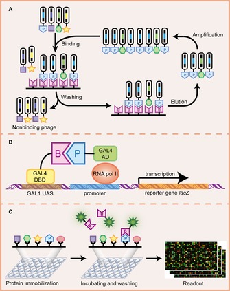
Illustration of some genetic methods for PPI detection. A) Phage display. A library of phage, each displaying a different protein including the prey, is exposed to a plate immobilized with the bait. After washing, phages displaying the prey bound to the bait will remain while nonbinding phages are removed. The remaining phages are then eluted, amplified by bacterial infection, and enriched in repeated selection cycles, that is, the “panning” process. B) The yeast two‐hybrid (Y2H) system. The binding domain (BD) and activation domain (AD) are two separate fragments of the transcription factor GAL4. They are fused to the bait and prey, respectively, where BD is responsible for binding to the upstream activating sequence (UAS) and AD is responsible for activation of transcription. The bait–prey interaction brings BD and AD into proximity to form an intact and functional transcriptional activator, which in turn recruits the basal transcriptional machinery and induces transcription of a downstream reporter gene lacZ. C) Protein microarray. A library of proteins is spotted onto a solid surface. This array is then incubated with a labelled bait. The interaction between the bait and the prey can be detected by a readout system employing a label‐based technique such as fluorescence.

The preferred systems that have been used for phage display include the filamentous M13 phage and the lytic T7 phage. M13 phage display provides easy manipulation in library construction but encounters misfolding problems as the displayed proteins are secreted through the periplasmin space of the E. coli membrane. While T7 phage display, with fusion proteins displayed on the C terminus of capsid protein 10B, does not suffer from such issues as the displayed protein released from the host cell through lysis.215 A high‐quality, large‐diversity phage display library constructed from designed synthetic oligonucleotides, cDNA, or open reading frames (ORFs), is an essential requirement for PPI screening. For example, Karkkainen et al. designed codon‐optimized genes encoding for 296 human SH3 domains and cloned them into a M13‐derived phagemid vector for objective identification of SH3 domains that bind to target proteins of interest.216 Lin et al. identified a kaposin A‐interacting protein by using a phage display human brain cDNA library.217 In general, phage display with cDNA libraries is inefficient and uncommon, as a cDNA library with unpredictable reading frames and stop codons can lead to inappropriate protein expression, and out‐of‐frame phage clones encoding unnatural short peptides trend to outgrow clones with correctly displayed sequences.218 ORF phage display solves this problem by eliminating non‐ORF clones and ensures that the majority of phage clones encode real proteins. For example, by developing a high‐quality ORF phage display, Caberoy et al. identified 16 new tubby‐binding proteins, most of which were validated by Y2H and pull‐down assay, eventually proved high accuracy rate of this technology.218

4.2.  Yeast two‐hybrid (Y2H) system and other two‐hybrid systems

A transcriptional activator in yeast GAL4 contains two distinct domains, a DNA‐binding domain (DBD) and an activation domain (AD), which independently are nonfunctional as a transcription factor, but reconstitute a functional GAL4 transcription factor when they are in close proximity.219 Inspired by this finding, Fields and Song first described the Y2H method in 1989.220 They fused two yeast proteins bait and prey to the DBD and AD of GAL4, respectively. As bait and prey were known to interact, co‐expression of these two hybrid proteins in yeast reconstituted proximity of the GAL4 domains, leading to transcription of a GAL1‐lacZ reporter gene that could be analyzed by β‐galactosidase activity measurement (Figure 3 B). Y2H is a powerful technique for identifying and analyzing PPIs in vivo. However, as Y2H requires the translocation of the interacting proteins into the nucleus, it′s not suitable for membrane proteins or proteins localized in other subcellular compartment. Other unsuited proteins include transcriptional activators, which produce spontaneous activation of the transcription of the reporter gene independent of bait–prey interaction. Moreover, Y2H cannot detect PPIs involving post‐translational modifications that do not take place in yeast.221

To circumvent the limitations of Y2H and extend its application, a number of variant two‐hybrid systems have been developed:

(1) The repressed transactivator (RTA) system was established for detection of interactions with transcriptional activator proteins.222 An auto‐activating bait protein is fused to DBD of GAL4, whereas prey is fused to the repression domain (RD) of a transcription repressor TUP1. Therefore, bait–prey interaction causes repression of a reporter gene. This method has been applied to screen for various transcriptional activators, such as VP16,222 c‐Myc,222, 223, 224 Mitf,225 and androgen receptor.226, 227, 228

(2) RNA polymerase III (Pol III) system can be used to assess the interactions between RNA polymerase II regulatory proteins and their partners, which cannot be analyzed by the classic, RNA polymerase II‐dependent Y2H. In the RNA Pol III system, protein prey is fused to τ138p, which can activate RNA polymerase III‐mediated transcription.229

(3) Sos recruitment system (SRS) is based on the Ras signaling pathway instead of transcriptional regulation in classic Y2H. In SRS, bait is fused to mammalian Sos, and prey is fused to a membrane localization signal. Interaction between bait and prey results in Sos membrane localization and Ras activation, allows a Cdc25‐2 temperature sensitive yeast strain grow at the restrictive temperature.230 Since SRS does not depend on a transcriptional readout, it can study interactions involving transcriptional activators or repressors. Furthermore, it is suitable for identifying proteins that do not target well to the nucleus or undergo post‐translational modifications in the cytoplasm.

(4) An improved version of SRS is the Ras recruitment system (RRS), in which bait is fused to constitutively active mammalian Ras instead of Sos.231

(5) The G protein fusion system allows the interaction between an integral membrane protein bait and a soluble prey to be studied. By this method, the prey fused to the G protein γ‐subunit is localized at the membrane upon interaction with bait, leading to the disruption of G protein signaling and downstream transcriptional events.232

(6) SCINEX‐P system is developed to analysis interactions between extracellular or transmembrane proteins in the endoplasmic reticulum (ER), in which bait and prey are fused to truncated Ire1p. Bait–prey interaction causes dimerization of Ire1p, which activates unfolded protein response signaling, leading to Hac1p‐dependent activation of reporter genes.233

(7) Reverse two‐hybrid system is an upside‐down version of Y2H, in which disruption of the bait–prey interaction decreases the expression of a counter‐selectable reporter gene, such as URA3,234 CYH2235 and GAL1,236 and allows cell growth under selective conditions. This method facilitates the detection of dissociation of PPIs, and the selection of small‐molecule inhibitors against PPIs that could be developed as therapeutic agents.237

(8) Bacterial two‐hybrid system using E. coli as a host organism offers some advantages over Y2H, including ease of use, lack of cellular compartmentalization, rapid library screening due to high transformation efficiency, and fast growth rate observed with E. coli, and increased sensitivity due to the absence of endogenous proteins that compete for the interactions.168 A number of bacterial two‐hybrid systems have been studied, which are based on recruitment of RNA polymerase to activate a lacZ reporter gene,238 complementation of signaling enzymes such as adenylate cyclase,239 dimerization of LexA derivatives to reconstitute a functional repressor,240 and reconstitution of polyhydroxyalkanoates synthesis regulatory protein PhaR.241

(9) Mammalian two‐hybrid system allows for the studies of interactions of proteins in native physiological context with proper folding and post‐translational modifications. One unique system termed MAPPIT (mammalian protein–protein interaction trap) is founded on type I cytokine signal transduction, in which bait–prey interaction restores JAK–STAT signaling and finally induces transcription of a reporter gene coupled to a STAT‐dependent promoter.242 This approach has been well validated for large‐scale interactomics studies and high‐throughput drug screening.243

(10) Fluorescent two‐hybrid (F2H) assay takes advantage of cell lines harboring a stable integration of a lac operator array. In such an assay, a fluorescently labeled bait is fused to a lac repressor and then immobilized. Interaction between the bait and a differently labeled prey leads to co‐localization of fluorescent signals. This technique enables visualization and analysis of PPIs from different subcellular compartments including nucleus, cytoplasm, and mitochondria in living cells in real time.244, 245, 246

4.3.  Protein microarray

Protein microarray technology is a high‐throughput method that allows simultaneous analysis of thousands of proteins arrayed at high density on a solid surface (Figure 3 C). Among various forms of protein microarrays, functional protein microarray is constructed by immobilizing large number of full‐length functional proteins or protein domains onto the chips, which is used to study biochemical properties and activities of an entire proteome in a single experiment including assessing PPIs.247 A major breakthrough came from a study by Zhu et al.248 They cloned 5800 yeast ORFs, expressed and purified their corresponding proteins with His*6 fusion tag, spotted these proteins onto nickel‐coated slides, and finally generated the first proteome microarray containing 80 % yeast proteins. After incubating the microarrays with biotinylated calmodulin and Cy3‐labeled streptavidin, calmodulin‐interacting proteins were identified by fluorescence signal detection. Since then, proteome microarrays have been successfully employed for identification of protein interaction partners, that is, to discover calmodulin‐binding proteins with microarray containing 1133 proteins in Arabidopsis thaliana, 249 to investigate novel links of protein kinases to distinct cellular pathways using yeast proteome microarray composed of ∼4200 GST fusion yeast proteins,250 to profile the BAG3 interactome by using a human proteome microarray comprising ∼17 000 unique full‐length human ORFs.251

The core technologies and corresponding challenges in functional protein microarray include:

(1) Construction of a comprehensive expression clone library. Although proteome microarrays have been fabricated from the proteomes of yeast,248, 250 E. coli,252 coronavirus,253 Arabidopsis thaliana, 249 and human,251, 254 expression‐ready ORF collections for other species are highly desired.

(2) High‐throughput protein production, including protein expression and purification. Expression in a homologous system is ideal for analysis of yeast and E. coli proteins, because these proteins are in their natural environment and thus fold properly.248, 252 While for most eukaryotic proteins, expression in a heterologous system such as in E. coli can cause solubility problems due to improper folding and the loss of native post‐translational modification. For protein purification, affinity tags such as His*6, GST, FLAG, maltose binding protein, are fused to either the C or N terminus of these proteins, which can facilitate purification by using specific resins. As the traditional cloning–expressing—purification–printing approach is time consuming and labor intensive, a nucleic acid programmable protein array (NAPPA) was developed. It spots expression plasmids on the chip and uses a mammalian cell‐free expression system to allow the proteins to be expressed and immobilized in situ through affinity tags without requiring purification.255

(3) Protein immobilization. As proteins have a 3D structure that is critical to their function, it is necessary to develop effective protein immobilization methods that do not cause activity loss or incorrect orientation of the capture proteins. To this end, various methods have been developed, such as noncovalent absorption,256 covalent binding by chemical bonding,257, 258 and affinity capture.248

(4) Detection method. Readout systems based on a label‐dependent strategy, such as fluorescence, radioactivity, chemiluminescence, enzymatic signal amplification, or label‐free strategy such as surface plasmon resonance, mass spectrometry, atomic force microscopy, can be used to detect signals within each microspot.259

5.  Summary & Outlook

The human interactome is estimated to contain ∼170 000 binary PPI pairs, the majority of which remains to be explored.260 Revealing the temporal and spatial relationships between interacting proteins will certainly help to establish a better understanding of the molecular mechanism of biological processes as well as the identification of a wider range of potential targets for drug discovery. Biophysical methods, such as AUC and ITC, are often based on long‐standing physical principles. They have started to show good performance in studying the hydrodynamic and thermodynamic aspects of PPIs owing to dramatic improvements in instrumentation. Biochemical methods, such as affinity chromatography, are also frequently applied together with MS techniques to identify the binding partners of the protein of interest. During the past decade, genomics revolution has assisted in the construction of genome‐scale cDNA and ORF collections, which facilitates PPI identification and PPI network mapping on a large scale with high‐throughput genetic methods, such as Y2H, phage display, and protein microarray. It should be kept in mind that all methods have their own limitations, and these can lead to false positives and negatives in detection. Therefore, validation of PPIs using methods based on different techniques is recommended to produce reliable results. For example, potential PPIs discovered by genetic methods can be further confirmed by biochemical assays. Finally, it is important to note that, since experimental measurements have generated a wealth of data, there is an increasing demand for publicly accessible databases that collect and record such data in some standard formats. More powerful bioinformatic tools are also much needed to convert raw data into useful knowledge.

Biographical Information

Mi Zhou studied molecular biology at Tongji University (Shanghai, China) and received a Master's degree in 2010. Since then, she has been working as a Research Associate in Prof. Renxiao Wang′s group at the Shanghai Institute of Organic Chemistry, Chinese Academy of Sciences. Her research focuses on experimental characterization of small‐molecule regulators of protein–protein interactions.

Biographical Information

Qing Li received her Master's degree in biochemistry and molecular biology in 2014 from the Shanghai Normal University (Shanghai, China). Since then, she has been working as a Research Associate in Prof. Renxiao Wang′s group. Her research focuses on characterizing the biological activities of small molecules with cell‐based assays.

Biographical Information

Prof. Renxiao Wang received both his B.S. degree (1994) and Ph.D. degree (1999) from Peking University (Beijing, China). Prof. Wang carried out his postdoctoral research at the University of California, Los Angeles (Los Angeles, USA) and Georgetown University (Washington, D.C., USA), and also worked as a research investigator at the University of Michigan Medical School (Ann Arbor, USA). In 2005, he joined the Shanghai Institute of Organic Chemistry as a principal investigator. His main research interests involve understanding how small organic molecules regulate their biological targets through molecular modelling approaches. In 2012, Prof. Wang received the Corwin Hansch Award from the Cheminformatics and QSAR Society in recognition of his contributions to the field of computer‐aided drug design.

M. Zhou, Q. Li, R. Wang, ChemMedChem 2016, 11, 738.

References

- 1. Ezkurdia I., Juan D., Rodriguez J. M., Frankish A., Diekhans M., Harrow J., Vazquez J., Valencia A., Tress M. L., Hum. Mol. Genet. 2014, 23, 5866–5878. [DOI] [PMC free article] [PubMed] [Google Scholar]
- 2. Berggård T., Linse S., James P., Proteomics 2007, 7, 2833–2842. [DOI] [PubMed] [Google Scholar]
- 3. Braun P., Gingras A. C., Proteomics 2012, 12, 1478–1498. [DOI] [PubMed] [Google Scholar]
- 4. Pelletier J., Sidhu S., Curr. Opin. Biotechnol. 2001, 12, 340–347. [DOI] [PubMed] [Google Scholar]
- 5. Vidal M., Cusick M. E., Barabasi A. L., Cell 2011, 144, 986–998. [DOI] [PMC free article] [PubMed] [Google Scholar]
- 6. Ruffner H., Bauer A., Bouwmeester T., Drug Discovery Today 2007, 12, 709–716. [DOI] [PubMed] [Google Scholar]
- 7. Tse C., Shoemaker A. R., Adickes J., Anderson M. G., Chen J., Jin S., Johnson E. F., Marsh K. C., Mitten M. J., Nimmer P., Roberts L., Tahir S. K., Xiao Y., Yang X., Zhang H., Fesik S., Rosenberg S. H., Elmore S. W., Cancer Res. 2008, 68, 3421–3428. [DOI] [PubMed] [Google Scholar]
- 8. Vu B. T., Vassilev L., Curr. Top. Microbiol. Immunol. 2011, 348, 151–172. [DOI] [PubMed] [Google Scholar]
- 9. Dorr P., Westby M., Dobbs S., Griffin P., Irvine B., Macartney M., Mori J., Rickett G., Smith-Burchnell C., Napier C., Webster R., Armour D., Price D., Stammen B., Wood A., Perros M., Antimicrob. Agents Chemother. 2005, 49, 4721–4732. [DOI] [PMC free article] [PubMed] [Google Scholar]
- 10. Peerlinck K., De Lepeleire I., Goldberg M., Farrell D., Barrett J., Hand E., Panebianco D., Deckmyn H., Vermylen J., Arnout J., Circulation 1993, 88, 1512–1517. [DOI] [PubMed] [Google Scholar]
- 11. Uvebrant K., da Graca Thrige D., Rosen A., Akesson M., Berg H., Walse B., Bjork P., J. Biomol. Screening 2007, 12, 464–472. [DOI] [PubMed] [Google Scholar]
- 12. Gul S., Hadian K., Expert Opin. Drug Discovery 2014, 9, 1393–1404. [DOI] [PubMed] [Google Scholar]
- 13. Fischer G., Rossmann M., Hyvonen M., Curr. Opin. Biotechnol. 2015, 35, 78–85. [DOI] [PMC free article] [PubMed] [Google Scholar]
- 14. Arkin M. R., Tang Y., Wells J. A., Chem. Biol. 2014, 21, 1102–1114. [DOI] [PMC free article] [PubMed] [Google Scholar]
- 15. Neduva V., Russell R. B., FEBS Lett. 2005, 579, 3342–3345. [DOI] [PubMed] [Google Scholar]
- 16. Tompa P., Davey N. E., Gibson T. J., Babu M. M., Mol. Cell 2014, 55, 161–169. [DOI] [PubMed] [Google Scholar]
- 17. Perrin F., J. Phys. Radium. 1926, 7, 390–401. [Google Scholar]
- 18. Du Y. in Protein–Protein Interactions (Eds.: C. L. Meyerkord, H. Fu), Vol. 1278 of the series Methods in Molecular Biology (Series Ed.: J. M. Walker), Springer, New York, 2015, p. 529–544. [DOI] [PubMed] [Google Scholar]
- 19. Weiel J., Hershey J. W., Biochemistry 1981, 20, 5859–5865. [DOI] [PubMed] [Google Scholar]
- 20. Weiel J., Hershey J. W., J. Biol. Chem. 1982, 257, 1215–1220. [PubMed] [Google Scholar]
- 21. Kim Y. T., Tabor S., Churchich J. E., Richardson C. C., J. Biol. Chem. 1992, 267, 15032–15040. [PubMed] [Google Scholar]
- 22. Lea W. A., Simeonov A., Expert Opin. Drug Discovery 2011, 6, 17–32. [DOI] [PMC free article] [PubMed] [Google Scholar]
- 23. Knight S. M., Umezawa N., Lee H. S., Gellman S. H., Kay B. K., Anal. Biochem. 2002, 300, 230–236. [DOI] [PubMed] [Google Scholar]
- 24. Kenny C. H., Ding W., Kelleher K., Benard S., Dushin E. G., Sutherland A. G., Mosyak L., Kriz R., Ellestad G., Anal. Biochem. 2003, 323, 224–233. [DOI] [PubMed] [Google Scholar]
- 25. Hassig C. A., Zeng F. Y., Kung P., Kiankarimi M., Kim S., Diaz P. W., Zhai D., Welsh K., Morshedian S., Su Y., O′Keefe B., Newman D. J., Rusman Y., Kaur H., Salomon C. E., Brown S. G., Baire B., Michel A. R., Hoye T. R., Francis S., Georg G. I., Walters M. A., Divlianska D. B., Roth G. P., Wright A. E., Reed J. C., J. Biomol. Screening 2014, 19, 1201–1211. [DOI] [PMC free article] [PubMed] [Google Scholar]
- 26. Owicki J. C., J. Biomol. Screening 2000, 5, 297–306. [DOI] [PubMed] [Google Scholar]
- 27. Madeira A., Ohman E., Nilsson A., Sjogren B., Andren P. E., Svenningsson P., Nat. Protoc. 2009, 4, 1023–1037. [DOI] [PubMed] [Google Scholar]
- 28. Boozer C., Kim G., Cong S., Guan H., Londergan T., Curr. Opin. Biotechnol. 2006, 17, 400–405. [DOI] [PubMed] [Google Scholar]
- 29. Nguyen H. H., Park J., Kang S., Kim M., Sensors 2015, 15, 10481–10510. [DOI] [PMC free article] [PubMed] [Google Scholar]
- 30. McDonnell J. M., Curr. Opin. Chem. Biol. 2001, 5, 572–577. [DOI] [PubMed] [Google Scholar]
- 31. Rich R. L., Myszka D. G., Curr. Opin. Biotechnol. 2000, 11, 54–61. [DOI] [PubMed] [Google Scholar]
- 32. Oesterreicher S., Blum W. F., Schmidt B., Braulke T., Kubler B., J. Biol. Chem. 2005, 280, 9994–10000. [DOI] [PubMed] [Google Scholar]
- 33. Vernon-Wilson E. F., Kee W. J., Willis A. C., Barclay A. N., Simmons D. L., Brown M. H., Eur. J. Immunol. 2000, 30, 2130–2137. [DOI] [PubMed] [Google Scholar]
- 34. Rogstam A., Linse S., Lindqvist A., James P., Wagner L., Berggard T., Biochem. J. 2007, 401, 353–363. [DOI] [PMC free article] [PubMed] [Google Scholar]
- 35. Homola J., Anal. Bioanal. Chem. 2003, 377, 528–539. [DOI] [PubMed] [Google Scholar]
- 36. Yuk J. S., Kim H. S., Jung J. W., Jung S. H., Lee S. J., Kim W. J., Han J. A., Kim Y. M., Ha K. S., Biosens. Bioelectron. 2006, 21, 1521–1528. [DOI] [PubMed] [Google Scholar]
- 37. Remy-Martin F., El Osta M., Lucchi G., Zeggari R., Leblois T., Bellon S., Ducoroy P., Boireau W., Anal. Bioanal. Chem. 2012, 404, 423–432. [DOI] [PubMed] [Google Scholar]
- 38. Thompson P. M., Beck M. R., Campbell S. L., in Protein–Protein Interactions (Eds.: C.L. Meyerkord, H. Fu ), Vol. 1278 of the series Methods in Molecular Biology (Series Ed.: J. M. Walker), Springer, New York, 2015, p. 267–279. [Google Scholar]
- 39. Garrett D. S., Seok Y. J., Peterkofsky A., Clore G. M., Gronenborn A. M., Biochemistry 1997, 36, 4393–4398. [DOI] [PubMed] [Google Scholar]
- 40. Greene M. K., Maskos K., Landry S. J., Proc. Natl. Acad. Sci. USA 1998, 95, 6108–6113. [DOI] [PMC free article] [PubMed] [Google Scholar]
- 41. Garrett D. S., Seok Y. J., Peterkofsky A., Gronenborn A. M., Clore G. M., Nat. Struct. Biol. 1999, 6, 166–173. [DOI] [PubMed] [Google Scholar]
- 42. Dhalluin C., Yan K. S., Plotnikova O., Lee K. W., Zeng L., Kuti M., Mujtaba S., Goldfarb M. P., Zhou M. M., Mol. Cell 2000, 6, 921–929. [DOI] [PMC free article] [PubMed] [Google Scholar]
- 43. Clore G. M., Tang C., Iwahara J., Curr. Opin. Struct. Biol. 2007, 17, 603–616. [DOI] [PMC free article] [PubMed] [Google Scholar]
- 44. Tang C., Iwahara J., Clore G. M., Nature 2006, 444, 383–386. [DOI] [PubMed] [Google Scholar]
- 45. Chen K., Tjandra N., Top. Curr. Chem. 2011, 326, 47–67. [DOI] [PMC free article] [PubMed] [Google Scholar]
- 46. Jensen M. R., Ortega-Roldan J. L., Salmon L., van Nuland N., Blackledge M., Eur. Biophys. J. 2011, 40, 1371–1381. [DOI] [PubMed] [Google Scholar]
- 47. O′Connell M. R., Gamsjaeger R., Mackay J. P., Proteomics 2009, 9, 5224–5232. [DOI] [PubMed] [Google Scholar]
- 48. Miao Y., Cross T. A., Curr. Opin. Struct. Biol. 2013, 23, 919–928. [DOI] [PMC free article] [PubMed] [Google Scholar]
- 49. Maldonado A. Y., Burz D. S., Shekhtman A., Prog. Nucl. Magn. Reson. Spectrosc. 2011, 59, 197–212. [DOI] [PMC free article] [PubMed] [Google Scholar]
- 50. Ranjbar B., Gill P., Chem. Biol. Drug Des. 2009, 74, 101–120. [DOI] [PubMed] [Google Scholar]
- 51. Reed J., Kinzel V., Biochemistry 1984, 23, 1357–1362. [DOI] [PubMed] [Google Scholar]
- 52. Greenfield N. J., Fowler V. M., Biophys. J. 2002, 82, 2580–2591. [DOI] [PMC free article] [PubMed] [Google Scholar]
- 53. Greenfield N. J. in Protein–Protein Interactions (Ed.: H. Fu ), Vol. 261 of the series Methods in Molecular Biology (Series Ed.: J. M. Walker), Humana Press, 2004, p. 55–78. [DOI] [PubMed] [Google Scholar]
- 54. Honda S., Kobayashi N., Munekata E., Uedaira H., Biochemistry 1999, 38, 1203–1213. [DOI] [PubMed] [Google Scholar]
- 55. Cowieson N. P., Miles A. J., Robin G., Forwood J. K., Kobe B., Martin J. L., Wallace B. A., Proteins Struct. Funct. Bioinf. 2008, 70, 1142–1146. [DOI] [PubMed] [Google Scholar]
- 56. Wallace B. A., Janes R. W., Biochem. Soc. Trans. 2010, 38, 861–873. [DOI] [PubMed] [Google Scholar]
- 57. Greenfield N. J., Nat. Protoc. 2007, 1, 2527–2535. [DOI] [PMC free article] [PubMed] [Google Scholar]
- 58. Some D., Biophys. Rev. 2013, 5, 147–158. [DOI] [PMC free article] [PubMed] [Google Scholar]
- 59. Murphy R. M., Curr. Opin. Biotechnol. 1997, 8, 25–30. [DOI] [PubMed] [Google Scholar]
- 60. Kapoor N., Gupta R., Menon S. T., Folta-Stogniew E., Raleigh D. P., Sakmar T. P., J. Biol. Chem. 2010, 285, 31647–31660. [DOI] [PMC free article] [PubMed] [Google Scholar]
- 61. Attri A. K., Minton A. P., Anal. Biochem. 2005, 346, 132–138. [DOI] [PubMed] [Google Scholar]
- 62. Martos A., Alfonso C., Lopez-Navajas P., Ahijado-Guzmn R., Mingorance J., Minton A. P., Rivas G., Biochemistry 2010, 49, 10780–10787. [DOI] [PubMed] [Google Scholar]
- 63. Laue T., Drug Discovery Today Technol. 2004, 1, 309–315. [DOI] [PubMed] [Google Scholar]
- 64. Lebowitz J., Lewis M. S., Schuck P., Protein Sci. 2002, 11, 2067–2079. [DOI] [PMC free article] [PubMed] [Google Scholar]
- 65. Zhao H., Beckett D., J. Mol. Biol. 2008, 380, 223–236. [DOI] [PMC free article] [PubMed] [Google Scholar]
- 66. Walters C., Errington N., Rowe A. J., Harding S. E., Biochem. J. 2002, 364, 849–855. [DOI] [PMC free article] [PubMed] [Google Scholar]
- 67. Harding S. E., Rowe A. J., Biochem. Soc. Trans. 2010, 38, 901–907. [DOI] [PubMed] [Google Scholar]
- 68. Silkowski H., Davis S. J., Barclay A. N., Rowe A. J., Harding S. E., Byron O., Eur. Biophys. J. 1997, 25, 455–462. [DOI] [PubMed] [Google Scholar]
- 69. Philo J. S., Wen J., Wypych J., Schwartz M. G., Mendiaz E. A., Langley K. E., J. Biol. Chem. 1996, 271, 6895–6902. [DOI] [PubMed] [Google Scholar]
- 70. Rivas G., Minton A. P., Biochem. Soc. Trans. 2003, 31, 1015–1019. [DOI] [PubMed] [Google Scholar]
- 71. Ladbury J. E., Chowdhry B. Z., Chem. Biol. 1996, 3, 791–801. [DOI] [PubMed] [Google Scholar]
- 72. Falconer R. J., Penkova A., Jelesarov I., Collins B. M., J. Mol. Recognit. 2010, 23, 395–413. [DOI] [PubMed] [Google Scholar]
- 73. Ababou A., Ladbury J. E., J. Mol. Recognit. 2007, 20, 4–14. [DOI] [PubMed] [Google Scholar]
- 74. Pierce M. M., Raman C. S., Nall B. T., Methods 1999, 19, 213–221. [DOI] [PubMed] [Google Scholar]
- 75. Roselin L. S., Lin M. S., Lin P. H., Chang Y., Chen W. Y., Biotechnol. J. 2010, 5, 85–98. [DOI] [PubMed] [Google Scholar]
- 76. Sundberg E. J., Urrutia M., Braden B. C., Isern J., Tsuchiya D., Fields B. A., Malchiodi E. L., Tormo J., Schwarz F. P., Mariuzza R. A., Biochemistry 2000, 39, 15375–15387. [DOI] [PubMed] [Google Scholar]
- 77. Bello M., Pérez-Hernández G., Fernández-Velasco D. A., Arreguín-Espinosa R., García-Hernández E., Proteins Struct. Funct. Bioinf. 2008, 70, 1475–1487. [DOI] [PubMed] [Google Scholar]
- 78. Krachler A. M., Sharma A., Cauldwell A., Papadakos G., Kleanthous C., J. Mol. Biol. 2010, 403, 270–285. [DOI] [PubMed] [Google Scholar]
- 79. Privalov P. L., Dragan A. I., Biophys. Chem. 2007, 126, 16–24. [DOI] [PubMed] [Google Scholar]
- 80. Chiu M. H., Prenner E. J., J. Pharm. Bioallied Sci. 2011, 3, 39–59. [DOI] [PMC free article] [PubMed] [Google Scholar]
- 81. Mitkevich V. A., Schulga A. A., Ermolyuk Y. S., Lobachov V. M., Chekhov V. O., Yakovlev G. I., Hartley R. W., Nick Pace C., Kirpichnikov M. P., Makarov A. A., Biophys. Chem. 2003, 105, 383–390. [DOI] [PubMed] [Google Scholar]
- 82. Jung H. I., Bowden S. J., Cooper A., Perham R. N., Protein Sci. 2002, 11, 1091–1100. [DOI] [PMC free article] [PubMed] [Google Scholar]
- 83. Cooper A. in Protein Targeting Protocols (Ed.: R. A. Clegg), Vol. 88 of the series Methods in Molecular Biology (Series Ed.: J. M. Walker), Humana Press, 1998, p. 11–22. [Google Scholar]
- 84. Wienken C. J., Baaske P., Rothbauer U., Braun D., Duhr S., Nat. Commun. 2010, 1, 100. [DOI] [PubMed] [Google Scholar]
- 85. Seidel S. A., Dijkman P. M., Lea W. A., van den Bogaart G., Jerabek-Willemsen M., Lazic A., Joseph J. S., Srinivasan P., Baaske P., Simeonov A., Katritch I., Melo F. A., Ladbury J. E., Schreiber G., Watts A., Braun D., Duhr S., Methods 2013, 59, 301–315. [DOI] [PMC free article] [PubMed] [Google Scholar]
- 86. Mao Y., Yu L., Yang R., Qu L. B., Harrington Pde B., Talanta 2015, 132, 894–901. [DOI] [PubMed] [Google Scholar]
- 87. Jerabek-Willemsen M., Wienken C. J., Braun D., Baaske P., Duhr S., Assay Drug Dev. Technol. 2011, 9, 342–353. [DOI] [PMC free article] [PubMed] [Google Scholar]
- 88. Arbel N., Ben-Hail D., Shoshan-Barmatz V., J. Biol. Chem. 2012, 287, 23152–23161. [DOI] [PMC free article] [PubMed] [Google Scholar]
- 89. Lin C. C., Melo F. A., Ghosh R., Suen K. M., Stagg L. J., Kirkpatrick J., Arold S. T., Ahmed Z., Ladbury J. E., Cell 2012, 149, 1514–1524. [DOI] [PubMed] [Google Scholar]
- 90. Jerabek-Willemsen M., André T., Wanner R., Roth H. M., Duhr S., Baaske P., Breitsprecher D., J. Mol. Struct. 2014, 1077, 101–113. [Google Scholar]
- 91. Förster T., Ann. Phys. 1948, 437, 55–75. [Google Scholar]
- 92. Pollok B. A., Heim R., Trends Cell Biol. 1999, 9, 57–60. [DOI] [PubMed] [Google Scholar]
- 93. Nguyen A. W., Daugherty P. S., Nat. Biotechnol. 2005, 23, 355–360. [DOI] [PubMed] [Google Scholar]
- 94. Karasawa S., Araki T., Nagai T., Mizuno H., Miyawaki A., Biochem. J. 2004, 381, 307–312. [DOI] [PMC free article] [PubMed] [Google Scholar]
- 95. Aker J., Hesselink R., Engel R., Karlova R., Borst J. W., Visser A. J., de Vries S. C., Plant Physiol. 2007, 145, 339–350. [DOI] [PMC free article] [PubMed] [Google Scholar]
- 96. Adjobo-Hermans M. J., Goedhart J., T. W. Gadella, Jr. , J. Cell. Sci. 2006, 119, 5087–5097. [DOI] [PubMed] [Google Scholar]
- 97. Hoffmann C., Gaietta G., Bunemann M., Adams S. R., Oberdorff-Maass S., Behr B., Vilardaga J. P., Tsien R. Y., Ellisman M. H., Lohse M. J., Nat. Methods 2005, 2, 171–176. [DOI] [PubMed] [Google Scholar]
- 98. Song Y., Madahar V., Liao J., Ann. Biomed. Eng. 2011, 39, 1224–1234. [DOI] [PMC free article] [PubMed] [Google Scholar]
- 99. Song Y., Liao J., Assay Drug Dev. Technol. 2012, 10, 336–343. [DOI] [PMC free article] [PubMed] [Google Scholar]
- 100. Mahajan N. P., Linder K., Berry G., Gordon G. W., Heim R., Herman B., Nat. Biotechnol. 1998, 16, 547–552. [DOI] [PubMed] [Google Scholar]
- 101. Xia Z., Zhou Q., Lin J., Liu Y., J Biol Chem. 2001, 276, 1766–1771. [DOI] [PubMed] [Google Scholar]
- 102. Day R. N., Davidson M. W., Bioessays 2012, 34, 341–350. [DOI] [PMC free article] [PubMed] [Google Scholar]
- 103. Periasamy A., J. Biomed. Opt. 2001, 6, 287–291. [DOI] [PubMed] [Google Scholar]
- 104. Piston D. W., Kremers G. J., Trends Biochem. Sci. 2007, 32, 407–414. [DOI] [PubMed] [Google Scholar]
- 105. Youvan D. C., Silva C. M., Bylina E. J., Coleman W. J., Dilworth M. R., Yang M. M., Biotechnology et alia 1997, 3, 1–18. [Google Scholar]
- 106. Hoppe A., Christensen K., Swanson J. A., Biophys. J. 2002, 83, 3652–3664. [DOI] [PMC free article] [PubMed] [Google Scholar]
- 107. Kenworthy A. K., Edidin M., J. Cell Biol. 1998, 142, 69–84. [DOI] [PMC free article] [PubMed] [Google Scholar]
- 108. Chan F. K., Siegel R. M., Zacharias D., Swofford R., Holmes K. L., Tsien R. Y., Lenardo M. J., Cytometry 2001, 44, 361–368. [DOI] [PubMed] [Google Scholar]
- 109. Wouters F. S., Bastiaens P. I., Wirtz K. W., Jovin T. M., EMBO J. 1998, 17, 7179–7189. [DOI] [PMC free article] [PubMed] [Google Scholar]
- 110. T. W. Gadella, Jr. , Jovin T. M., Clegg R. M., Biophys. Chem. 1993, 48, 221–239. [Google Scholar]
- 111. Ng T., Squire A., Hansra G., Bornancin F., Prevostel C., Hanby A., Harris W., Barnes D., Schmidt S., Mellor H., Bastiaens P. I., Parker P. J., Science 1999, 283, 2085–2089. [DOI] [PubMed] [Google Scholar]
- 112. Squire A., Bastiaens P. I., J. Microsc. 1999, 193, 36–49. [DOI] [PubMed] [Google Scholar]
- 113. Dickinson M. E., Bearman G., Tille S., Lansford R., Fraser S. E., Biotechniques 2001, 31, 1272, 1274–1276, 1278. [DOI] [PubMed] [Google Scholar]
- 114. Zimmermann T., Rietdorf J., Pepperkok R., FEBS Lett. 2003, 546, 87–92. [DOI] [PubMed] [Google Scholar]
- 115. Mattheyses A. L., Hoppe A. D., Axelrod D., Biophys. J. 2004, 87, 2787–2797. [DOI] [PMC free article] [PubMed] [Google Scholar]
- 116. Lidke D. S., Nagy P., Barisas B. G., Heintzmann R., Post J. N., Lidke K. A., Clayton A. H., Arndt-Jovin D. J., Jovin T. M., Biochem. Soc. Trans. 2003, 31, 1020–1027. [DOI] [PubMed] [Google Scholar]
- 117. He L., Olson D. P., Wu X., Karpova T. S., McNally J. G., Lipsky P. E., Cytometry Part A 2003, 55, 71–85. [DOI] [PubMed] [Google Scholar]
- 118. Dye B. T., Schell K., Miller D. J., Ahlquist P., Cytometry Part A 2005, 63, 77–86. [DOI] [PubMed] [Google Scholar]
- 119. Szalóki N., Doan-Xuan Q. M., Szöllősi J., Tóth K., Vámosi G., Bacsó Z., Cytometry Part A 2013, 83, 818–829. [DOI] [PubMed] [Google Scholar]
- 120. Glickman J. F., Wu X., Mercuri R., Illy C., Bowen B. R., He Y., Sills M., J. Biomol. Screening 2002, 7, 3–10. [DOI] [PubMed] [Google Scholar]
- 121. Breuer S., Espinola S., Morelli X., Torbett B. E., Arold S. T., Engels I. H., Curr. Chem. Genomics Transl. Med. 2013, 7, 16–20. [DOI] [PMC free article] [PubMed] [Google Scholar]
- 122. Gunther J. R., Du Y., Rhoden E., Lewis I., Revennaugh B., Moore T. W., Kim S. H., Dingledine R., Fu H., Katzenellenbogen J. A., J. Biomol. Screening 2009, 14, 181–193. [DOI] [PMC free article] [PubMed] [Google Scholar]
- 123. Du Y., Fu R. W., Lou B., Zhao J., Qui M., Khuri F. R., Fu H., Assay Drug Dev. Technol. 2013, 11, 367–381. [DOI] [PMC free article] [PubMed] [Google Scholar]
- 124. Gaborit N., Larbouret C., Vallaghe J., Peyrusson F., Bascoul-Mollevi C., Crapez E., Azria D., Chardes T., Poul M. A., Mathis G., Bazin H., Pelegrin A., J. Biol. Chem. 2011, 286, 11337–11345. [DOI] [PMC free article] [PubMed] [Google Scholar]
- 125. Kim B., Tarchevskaya S. S., Eggel A., Vogel M., Jardetzky T. S., Anal. Biochem. 2012, 431, 84–89. [DOI] [PMC free article] [PubMed] [Google Scholar]
- 126. Cottet M., Faklaris O., Maurel D., Scholler P., Doumazane E., Trinquet E., Pin J. P., Durroux T., Front. Endocrinol. 2012, 3, 92. [DOI] [PMC free article] [PubMed] [Google Scholar]
- 127. Fernández-Dueñas V., Llorente J., Gandía J., Borroto-Escuela D. O., Agnati L. F., Tasca C. I., Fuxe K., Ciruela F., Methods 2012, 57, 467–472. [DOI] [PubMed] [Google Scholar]
- 128. Bazin H., Trinquet E., Mathis G., J. Biotechnol. 2002, 82, 233–250. [DOI] [PubMed] [Google Scholar]
- 129. Bacart J., Corbel C., Jockers R., Bach S., Couturier C., Biotechnol. J. 2008, 3, 311–324. [DOI] [PubMed] [Google Scholar]
- 130. Boute N., Jockers R., Issad T., Trends Pharmacol. Sci. 2002, 23, 351–354. [DOI] [PubMed] [Google Scholar]
- 131. Xu Y., Piston D. W., Johnson C. H., Proc. Natl. Acad. Sci. USA 1999, 96, 151–156. [DOI] [PMC free article] [PubMed] [Google Scholar]
- 132. De A., Gambhir S. S., FASEB J. 2005, 19, 2017–2019. [DOI] [PubMed] [Google Scholar]
- 133. Pfleger K. D., Dromey J. R., Dalrymple M. B., Lim E. M., Thomas W. G., Eidne K. A., Cell. Signalling 2006, 18, 1664–1670. [DOI] [PubMed] [Google Scholar]
- 134. De A., Ray P., Loening A. M., Gambhir S. S., FASEB J. 2009, 23, 2702–2709. [DOI] [PMC free article] [PubMed] [Google Scholar]
- 135. Machleidt T., Woodroofe C. C., Schwinn M. K., Mendez J., Robers M. B., Zimmerman K., Otto P., Daniels D. L., Kirkland T. A., Wood K. V., ACS Chem. Biol. 2015, 10, 1797–1804. [DOI] [PubMed] [Google Scholar]
- 136. Xu X., Soutto M., Xie Q., Servick S., Subramanian C., von Arnim A. G., Johnson C. H., Proc. Natl. Acad. Sci. USA 2007, 104, 10264–10269. [DOI] [PMC free article] [PubMed] [Google Scholar]
- 137. De A., Loening A. M., Gambhir S. S., Cancer Res. 2007, 67, 7175–7183. [DOI] [PMC free article] [PubMed] [Google Scholar]
- 138. Ullman E. F., Kirakossian H., Singh S., Wu Z. P., Irvin B. R., Pease J. S., Switchenko A. C., Irvine J. D., Dafforn A., Skold C. N., Proc. Natl. Acad. Sci. USA 1994, 91, 5426–5430. [DOI] [PMC free article] [PubMed] [Google Scholar]
- 139. Eglen R. M., Reisine T., Roby P., Rouleau N., Illy C., Bossé R., Bielefeld M., Curr. Chem. Genomics 2008, 1, 2–10. [DOI] [PMC free article] [PubMed] [Google Scholar]
- 140. Zhang M., Wisniewski J. A., Ji H., Anal. Biochem. 2015, 469, 43–53. [DOI] [PubMed] [Google Scholar]
- 141. Wagstaff K. M., Rawlinson S. M., Hearps A. C., Jans D. A., J. Biomol. Screening 2011, 16, 192–200. [DOI] [PubMed] [Google Scholar]
- 142. Watson V. G., Drake K. M., Peng Y., Napper A. D., Assay Drug Dev. Technol. 2013, 11, 253–268. [DOI] [PMC free article] [PubMed] [Google Scholar]
- 143. Mackie D. I., Roman D. L., J. Biomol. Screening 2011, 16, 869–877. [DOI] [PMC free article] [PubMed] [Google Scholar]
- 144. Schorpp K., Rothenaigner I., Salmina E., Reinshagen J., Low T., Brenke J. K., Gopalakrishnan J., Tetko I. V., Gul S., Hadian K., J. Biomol. Screening 2014, 19, 715–726. [DOI] [PMC free article] [PubMed] [Google Scholar]
- 145. Sierecki E., Stevers L. M., Giles N., Polinkovsky M. E., Moustaqil M., Mureev S., Johnston W. A., Dahmer-Heath M., Skalamera D., Gonda T. J., Gabrielli B., Collins B. M., Alexandrov K., Gambin Y., Mol. Cell. Proteomics 2014, 13, 2233–2245. [DOI] [PMC free article] [PubMed] [Google Scholar]
- 146. Waller H., Chatterji U., Gallay P., Parkinson T., Targett-Adams P., J. Virol. Methods 2010, 165, 202–210. [DOI] [PMC free article] [PubMed] [Google Scholar]
- 147. Yegorova S., Chavaroche A. E., Rodriguez M. C., Minond D., Cudic M., Anal. Biochem. 2013, 439, 123–131. [DOI] [PubMed] [Google Scholar]
- 148. Michnick S. W., Ear P. H., Landry C., Malleshaiah M. K., Messier V. in Signal Transduction Protocols (Eds.: L. M. Luttrell, S. S. G. Ferguson), Vol. 756 of the series Methods in Molecular Biology (Series Ed.: J. M. Walker), Humana Press, 2011, p. 395–425. [DOI] [PubMed] [Google Scholar]
- 149. Remy I., Michnick S. W., Proc. Natl. Acad. Sci. USA 1999, 96, 5394–5399. [DOI] [PMC free article] [PubMed] [Google Scholar]
- 150. Park J. H., Back J. H., Hahm S. H., Shim H. Y., Park M. J., Ko S. I., Han Y. S., J. Microbiol. Biotechnol. 2007, 17, 1607–1615. [PubMed] [Google Scholar]
- 151. Rossi F., Charlton C. A., Blau H. M., Proc. Natl. Acad. Sci. USA 1997, 94, 8405–8410. [DOI] [PMC free article] [PubMed] [Google Scholar]
- 152. Ear P. H., Michnick S. W., Nat. Methods 2009, 6, 813–816. [DOI] [PubMed] [Google Scholar]
- 153. Johnsson N., Varshavsky A., Proc. Natl. Acad. Sci. USA 1994, 91, 10340–10344. [DOI] [PMC free article] [PubMed] [Google Scholar]
- 154. Ozawa T., Nogami S., Sato M., Ohya Y., Umezawa Y., Anal. Chem. 2000, 72, 5151–5157. [DOI] [PubMed] [Google Scholar]
- 155. Ozawa T., Kaihara A., Sato M., Tachihara K., Umezawa Y., Anal. Chem. 2001, 73, 2516–2521. [DOI] [PubMed] [Google Scholar]
- 156. Remy I., Michnick S. W., Proc. Natl. Acad. Sci. USA 2001, 98, 7678–7683. [DOI] [PMC free article] [PubMed] [Google Scholar]
- 157. Tarassov K., Messier V., Landry C. R., Radinovic S., Serna Molina M. M., Shames I., Malitskaya Y., Vogel J., Bussey H., Michnick S. W., Science 2008, 320, 1465–1470. [DOI] [PubMed] [Google Scholar]
- 158. Rochette S., Gagnon-Arsenault I., Diss G., Landry C. R., J. Proteomics 2014, 100, 25–36. [DOI] [PubMed] [Google Scholar]
- 159. Stagljar I., Korostensky C., Johnsson N., te Heesen S., Proc. Natl. Acad. Sci. USA 1998, 95, 5187–5192. [DOI] [PMC free article] [PubMed] [Google Scholar]
- 160. Wittke S., Lewke N., Muller S., Johnsson N., Mol. Biol. Cell 1999, 10, 2519–2530. [DOI] [PMC free article] [PubMed] [Google Scholar]
- 161. Rojo-Niersbach E., Morley D., Heck S., Lehming N., Biochem. J. 2000, 348, 585–590. [PMC free article] [PubMed] [Google Scholar]
- 162. Wellhausen A., Lehming N., FEBS Lett. 1999, 453, 299–304. [DOI] [PubMed] [Google Scholar]
- 163. Dunnwald M., Varshavsky A., Johnsson N., Mol. Biol. Cell 1999, 10, 329–344. [DOI] [PMC free article] [PubMed] [Google Scholar]
- 164. Cabantous S., Nguyen H. B., Pedelacq J. D., Koraichi F., Chaudhary A., Ganguly K., Lockard M. A., Favre G., Terwilliger T. C., Waldo G. S., Sci. Rep. 2013, 3, 2854. [DOI] [PMC free article] [PubMed] [Google Scholar]
- 165. Kerppola T. K., Nat. Protoc. 2006, 1, 1278–1286. [DOI] [PMC free article] [PubMed] [Google Scholar]
- 166. Remy I., Michnick S. W., Nat. Methods 2006, 3, 977–979. [DOI] [PubMed] [Google Scholar]
- 167. Misawa N., Kafi A. K., Hattori M., Miura K., Masuda K., Ozawa T., Anal. Chem. 2010, 82, 2552–2560. [DOI] [PubMed] [Google Scholar]
- 168. Stynen B., Tournu H., Tavernier J., Van Dijck P., Microbiol. Mol. Biol. Rev. 2012, 76, 331–382. [DOI] [PMC free article] [PubMed] [Google Scholar]
- 169. W. G. Kaelin, Jr. , Pallas D. C., DeCaprio J. A., Kaye F. J., Livingston D. M., Cell 1991, 64, 521–532. [DOI] [PubMed] [Google Scholar]
- 170. Shao H., Xu X., Jing N., Tweardy D. J., J. Immunol. 2006, 176, 2933–2941. [DOI] [PubMed] [Google Scholar]
- 171. Król E., van Kessel S. P., van Bezouwen L. S., Kumar N., Boekema E. J., Scheffers D. J., PLoS One 2012, 7, e43293. [DOI] [PMC free article] [PubMed] [Google Scholar]
- 172. Mochizuki Y., Kohno F., Nishigaki K., Nemoto N., Anal. Biochem. 2013, 434, 93–95. [DOI] [PubMed] [Google Scholar]
- 173. Schulte R., Talamas J., Doucet C., Hetzer M. W., PLoS One 2008, 3, e2061. [DOI] [PMC free article] [PubMed] [Google Scholar]
- 174. Patel S. S., Rexach M. F., Mol. Cell. Proteomics 2008, 7, 121–131. [DOI] [PubMed] [Google Scholar]
- 175. Rigaut G., Shevchenko A., Rutz B., Wilm M., Mann M., Seraphin B., Nat. Biotechnol. 1999, 17, 1030–1032. [DOI] [PubMed] [Google Scholar]
- 176. Butland G., Peregrin-Alvarez J. M., Li J., Yang W., Yang X., Canadien V., Starostine A., Richards D., Beattie B., Krogan N., Davey M., Parkinson J., Greenblatt J., Emili A., Nature 2005, 433, 531–537. [DOI] [PubMed] [Google Scholar]
- 177. Gavin A. C., Bosche M., Krause R., Grandi P., Marzioch M., Bauer A., Schultz J., Rick J. M., Michon A. M., Cruciat C. M., Remor M., Hofert C., Schelder M., Brajenovic M., Ruffner H., Merino A., Klein K., Hudak M., Dickson D., Rudi T., Gnau V., Bauch A., Bastuck S., Huhse B., Leutwein C., Heurtier M. A., Copley R. R., Edelmann A., Querfurth E., Rybin V., Drewes G., Raida M., Bouwmeester T., Bork P., Seraphin B., Kuster B., Neubauer G., Superti-Furga G., Nature 2002, 415, 141–147. [DOI] [PubMed] [Google Scholar]
- 178. Krogan N. J., Cagney G., Yu H., Zhong G., Guo X., Ignatchenko A., Li J., Pu S., Datta N., Tikuisis A. P., Punna T., Peregrin-Alvarez J. M., Shales M., Zhang X., Davey M., Robinson M. D., Paccanaro A., Bray J. E., Sheung A., Beattie B., Richards D. P., Canadien V., Lalev A., Mena F., Wong P., Starostine A., Canete M. M., Vlasblom J., Wu S., Orsi C., Collins S. R., Chandran S., Haw R., Rilstone J. J., Gandi K., Thompson N. J., Musso G., St Onge P., Ghanny S., Lam M. H., Butland G., Altaf-Ul A. M., Kanaya S., Shilatifard A., O′Shea E., Weissman J. S., Ingles C. J., Hughes T. R., Parkinson J., Gerstein M., Wodak S. J., Emili A., Greenblatt J. F., Nature 2006, 440, 637–643. [DOI] [PubMed] [Google Scholar]
- 179. Brajenovic M., Joberty G., Kuster B., Bouwmeester T., Drewes G., J. Biol. Chem. 2004, 279, 12804–12811. [DOI] [PubMed] [Google Scholar]
- 180. Jeronimo C., Forget D., Bouchard A., Li Q., Chua G., Poitras C., Therien C., Bergeron D., Bourassa S., Greenblatt J., Chabot B., Poirier G. G., Hughes T. R., Blanchette M., Price D. H., Coulombe B., Mol. Cell 2007, 27, 262–274. [DOI] [PMC free article] [PubMed] [Google Scholar]
- 181. Bouwmeester T., Bauch A., Ruffner H., Angrand P. O., Bergamini G., Croughton K., Cruciat C., Eberhard D., Gagneur J., Ghidelli S., Hopf C., Huhse B., Mangano R., Michon A. M., Schirle M., Schlegl J., Schwab M., Stein M. A., Bauer A., Casari G., Drewes G., Gavin A. C., Jackson D. B., Joberty G., Neubauer G., Rick J., Kuster B., Superti-Furga G., Nat. Cell Biol. 2004, 6, 97–105. [DOI] [PubMed] [Google Scholar]
- 182. Major M. B., Camp N. D., Berndt J. D., Yi X., Goldenberg S. J., Hubbert C., Biechele T. L., Gingras A. C., Zheng N., Maccoss M. J., Angers S., Moon R. T., Science 2007, 316, 1043–1046. [DOI] [PubMed] [Google Scholar]
- 183. Li Y., Biotechnol. Appl. Biochem. 2010, 55, 73–83. [DOI] [PubMed] [Google Scholar]
- 184. Phizicky E. M., Fields S., Microbiol. Rev. 1995, 59, 94–123. [DOI] [PMC free article] [PubMed] [Google Scholar]
- 185. Poetz O., Luckert K., Herget T., Joos T. O., Anal. Biochem. 2009, 395, 244–248. [DOI] [PubMed] [Google Scholar]
- 186. Markham K., Bai Y., Schmitt-Ulms G., Anal. Bioanal. Chem. 2007, 389, 461–473. [DOI] [PubMed] [Google Scholar]
- 187. Weng Z., Zhao Q. in Protein–Protein Interactions (Eds.: C. L. Meyerkord, H. Fu), Vol. 1278 of the series Methods in Molecular Biology (Series Ed.: J. M. Walker), Springer, New York, 2015, p. 341–352. [DOI] [PubMed] [Google Scholar]
- 188. Lv M., Zhu Y., Wang J., Zhang H., Wang X., Zuo T., Liu D., Zhang J., Wu J., Kong W., Yu X., Protein Expression Purif. 2013, 91, 112–118. [DOI] [PubMed] [Google Scholar]
- 189. Ponticelli S., Braca A., De Tommasi N., De Falco S., Planta Med. 2008, 74, 401–406. [DOI] [PubMed] [Google Scholar]
- 190. Biesiadecki B. J., Jin J. P., J. Biomed. biotechnol. 2011, 2011, 1–8. [DOI] [PMC free article] [PubMed] [Google Scholar]
- 191. Meng Y., High K., Antonello J., Washabaugh M. W., Zhao Q., Anal. Biochem. 2005, 345, 227–236. [DOI] [PubMed] [Google Scholar]
- 192. Arkin M. R., Glicksman M. A., Fu H., Havel J. J., Du Y. in Assay Guidance Manual [Internet], (Eds.: G. S. Sittampalam, N. P. Coussens, H. Nelson, M. Arkin, D. Auld, C. Austin, B. Bejeck, M. Glicksman, J. Inglese, P. W. Iversen, Z. Y. Li, J. McGee, O. McManus, L. Minor, A. Napper, J. M. Peltier, T. Riss, O. J. Trask, Jr., J. Weidner), Bethesda (MD), Eli Lilly & Co. and the Nantional Center for Advancing Translational Sciences, USA, 2004; available from: http://www.ncbi.nlm.nih.gov/books/NBK92000/. [Google Scholar]
- 193. Fredriksson S., Gullberg M., Jarvius J., Olsson C., Pietras K., Gustafsdottir S. M., Ostman A., Landegren U., Nat. Biotechnol. 2002, 20, 473–477. [DOI] [PubMed] [Google Scholar]
- 194. Söderberg O., Leuchowius K. J., Kamali-Moghaddam M., Jarvius M., Gustafsdottir S., Schallmeiner E., Gullberg M., Jarvius J., Landegren U., Genet. Eng. 2007, 28, 85–93. [DOI] [PubMed] [Google Scholar]
- 195. Koos B., Andersson L., Clausson C. M., Grannas K., Klaesson A., Cane G., Söderberg O., Curr. Top. Microbiol. Immunol. 2014, 377, 111–126. [DOI] [PubMed] [Google Scholar]
- 196. Gustafsdottir S. M., Schallmeiner E., Fredriksson S., Gullberg M., Söderberg O., Jarvius M., Jarvius J., Howell M., Landegren U., Anal. Biochem. 2005, 345, 2–9. [DOI] [PubMed] [Google Scholar]
- 197. Söderberg O., Gullberg M., Jarvius M., Ridderstrale K., Leuchowius K. J., Jarvius J., Wester K., Hydbring P., Bahram F., Larsson L. G., Landegren U., Nat. Methods 2006, 3, 995–1000. [DOI] [PubMed] [Google Scholar]
- 198. Bellucci A., Fiorentini C., Zaltieri M., Missale C., Spano P., in Exocytosis and Endocytosis (Ed.: A. I. Ivanov), Vol. 1174 of the series Methods in Molecular Biology (Series Ed.: J. M. Walker), Springer, New York, 2014, p. 397–405. [DOI] [PubMed] [Google Scholar]
- 199. Gauthier T., Claude-Taupin A., Delage-Mourroux R., Boyer-Guittaut M., Hervouet E., PLoS One 2015, 10, e0128701. [DOI] [PMC free article] [PubMed] [Google Scholar]
- 200. Leuchowius K. J., Weibrecht I., Landegren U., Gedda L., Söderberg O., Cytometry Part A 2009, 75, 833–839. [DOI] [PubMed] [Google Scholar]
- 201. Söderberg O., Leuchowius K. J., Gullberg M., Jarvius M., Weibrecht I., Larsson L. G., Landegren U., Methods 2008, 45, 227–232. [DOI] [PubMed] [Google Scholar]
- 202. Tang X., Bruce J. E. in Mass Spectrometry of Proteins and Peptides (Eds.: M. S. Lipton, L. Paša-Tolic), Vol. 492 of the series Methods in Molecular Biology (Series Ed.: J. M. Walker), Humana Press, 2009, p. 283–293. [DOI] [PubMed] [Google Scholar]
- 203. Miernyk J. A., Thelen J. J., Plant J. 2008, 53, 597–609. [DOI] [PubMed] [Google Scholar]
- 204. Weber P. J., Beck-Sickinger A. G., J. Pept. Res. 1997, 49, 375–383. [DOI] [PubMed] [Google Scholar]
- 205. Müller D. R., Schindler P., Towbin H., Wirth U., Voshol H., Hoving S., Steinmetz M. O., Anal. Chem. 2001, 73, 1927–1934. [DOI] [PubMed] [Google Scholar]
- 206. Bennett K. L., Kussmann M., Bjork P., Godzwon M., Mikkelsen M., Sorensen P., Roepstorff P., Protein Sci. 2000, 9, 1503–1518. [DOI] [PMC free article] [PubMed] [Google Scholar]
- 207. Sinz A., Wang K., Biochemistry 2001, 40, 7903–7913. [DOI] [PubMed] [Google Scholar]
- 208. Sinz A., Kalkhof S., Ihling C., J. Am. Soc. Mass Spectrom. 2005, 16, 1921–1931. [DOI] [PubMed] [Google Scholar]
- 209. Guerrero C., Tagwerker C., Kaiser P., Huang L., Mol. Cell. Proteomics 2006, 5, 366–378. [DOI] [PubMed] [Google Scholar]
- 210. Vasilescu J., Guo X., Kast J., Proteomics 2004, 4, 3845–3854. [DOI] [PubMed] [Google Scholar]
- 211. Smith G. P., Science 1985, 228, 1315–1317. [DOI] [PubMed] [Google Scholar]
- 212. Pande J., Szewczyk M. M., Grover A. K., Biotechnol. Adv. 2010, 28, 849–858. [DOI] [PubMed] [Google Scholar]
- 213. Hertveldt K., Belien T., Volckaert G., in Bacteriophages (Eds.: M. R. J. Clokie, A. M. Kropinski), Vol. 502 of the series Methods in Molecular Biology (Series Ed.: J. M. Walker), Humana Press, 2009, p. 321–339. [DOI] [PubMed] [Google Scholar]
- 214. Paschke M., Appl. Microbiol. Biotechnol. 2006, 70, 2–11. [DOI] [PubMed] [Google Scholar]
- 215. Sundell G. N., Ivarsson Y., BioMed Res. Int. 2014, 2014, 176172. [DOI] [PMC free article] [PubMed] [Google Scholar]
- 216. Kärkkäinen S., Hiipakka M., Wang J. H., Kleino I., Vähä-Jaakkola M., Renkema G. H., Liss M., Wagner R., Saksela K., EMBO Rep. 2006, 7, 186–191. [DOI] [PMC free article] [PubMed] [Google Scholar]
- 217. Lin C. W., Tu P. F., Hsiao N. W., Chang C. Y., Wan L., Lin Y. T., Chang H. W., J. Virol. Methods 2007, 143, 65–72. [DOI] [PubMed] [Google Scholar]
- 218. Caberoy N. B., Zhou Y., Jiang X., Alvarado G., Li W., J. Mol. Recognit. 2010, 23, 74–83. [DOI] [PMC free article] [PubMed] [Google Scholar]
- 219. Keegan L., Gill G., Ptashne M., Science 1986, 231, 699–704. [DOI] [PubMed] [Google Scholar]
- 220. Fields S., Song O., Nature 1989, 340, 245–246. [DOI] [PubMed] [Google Scholar]
- 221. Hamdi A., Colas P., Trends Pharmacol. Sci. 2012, 33, 109–118. [DOI] [PubMed] [Google Scholar]
- 222. Hirst M., Ho C., Sabourin L., Rudnicki M., Penn L., Sadowski I., Proc. Natl. Acad. Sci. USA 2001, 98, 8726–8731. [DOI] [PMC free article] [PubMed] [Google Scholar]
- 223. Huang A., Ho C. S., Ponzielli R., Barsyte-Lovejoy D., Bouffet E., Picard D., Hawkins C. E., Penn L. Z., Cancer Res. 2005, 65, 5607–5619. [DOI] [PubMed] [Google Scholar]
- 224. Pineda-Lucena A., Ho C. S., Mao D. Y., Sheng Y., Laister R. C., Muhandiram R., Lu Y., Seet B. T., Katz S., Szyperski T., Penn L. Z., Arrowsmith C. H., J. Mol. Biol. 2005, 351, 182–194. [DOI] [PubMed] [Google Scholar]
- 225. Schwarz T., Sohn C., Kaiser B., Jensen E. D., Mansky K. C., J. Cell. Biochem. 2010, 109, 967–974. [DOI] [PMC free article] [PubMed] [Google Scholar]
- 226. Wafa L. A., Cheng H., Rao M. A., Nelson C. C., Cox M., Hirst M., Sadowski I., Rennie P. S., Biochem. J. 2003, 375, 373–383. [DOI] [PMC free article] [PubMed] [Google Scholar]
- 227. Ray M. R., Wafa L. A., Cheng H., Snoek R., Fazli L., Gleave M., Rennie P. S., Int. J. Cancer 2006, 118, 1108–1119. [DOI] [PubMed] [Google Scholar]
- 228. Tavassoli P., Wafa L. A., Cheng H., Zoubeidi A., Fazli L., Gleave M., Snoek R., Rennie P. S., Mol. Endocrinol. 2010, 24, 696–708. [DOI] [PMC free article] [PubMed] [Google Scholar]
- 229. Marsolier M. C., Prioleau M. N., Sentenac A., J. Mol. Biol. 1997, 268, 243–249. [DOI] [PubMed] [Google Scholar]
- 230. Aronheim A., Zandi E., Hennemann H., Elledge S. J., Karin M., Mol. Cell. Biol. 1997, 17, 3094–3102. [DOI] [PMC free article] [PubMed] [Google Scholar]
- 231. Broder Y. C., Katz S., Aronheim A., Curr. Biol. 1998, 8, 1121–1124. [DOI] [PubMed] [Google Scholar]
- 232. Ehrhard K. N., Jacoby J. J., Fu X. Y., Jahn R., Dohlman H. G., Nat. Biotechnol. 2000, 18, 1075–1079. [DOI] [PubMed] [Google Scholar]
- 233. Urech D. M., Lichtlen P., Barberis A., Biochim. Biophys. Acta. 2003, 1622, 117–127. [DOI] [PubMed] [Google Scholar]
- 234. Vidal M., Brachmann R. K., Fattaey A., Harlow E., Boeke J. D., Proc. Natl. Acad. Sci. USA 1996, 93, 10315–10320. [DOI] [PMC free article] [PubMed] [Google Scholar]
- 235. Leanna C. A., Hannink M., Nucleic Acids Res. 1996, 24, 3341–3347. [DOI] [PMC free article] [PubMed] [Google Scholar]
- 236. Gunde T., Tanner S., Auf der Maur A., Petrascheck M., Barberis A., Biotechniques 2004, 37, 844–852. [DOI] [PubMed] [Google Scholar]
- 237. Huang J., Schreiber S. L., Proc. Natl. Acad. Sci. USA 1997, 94, 13396–13401. [DOI] [PMC free article] [PubMed] [Google Scholar]
- 238. Joung J. K., Ramm E. I., Pabo C. O., Proc. Natl. Acad. Sci. USA 2000, 97, 7382–7387. [DOI] [PMC free article] [PubMed] [Google Scholar]
- 239. Battesti A., Bouveret E., Methods 2012, 58, 325–334. [DOI] [PubMed] [Google Scholar]
- 240. Dimitrova M., Younès-Cauet G., Oertel-Buchheit P., Porte D., Schnarr M., Granger-Schnarr M., Mol. Gen. Genet. 1998, 257, 205–212. [DOI] [PubMed] [Google Scholar]
- 241. Wang Z. H., Ma P., Chen J., Zhang J., Chen C. B., Chen G. Q., Microb. Cell Fact. 2011, 10, 21. [DOI] [PMC free article] [PubMed] [Google Scholar]
- 242. Eyckerman S., Verhee A., der Heyden J. V., Lemmens I., Ostade X. V., Vandekerckhove J., Tavernier J., Nat. Cell Biol. 2001, 3, 1114–1119. [DOI] [PubMed] [Google Scholar]
- 243. Lievens S., Peelman F., De Bosscher K., Lemmens I., Tavernier J., Cytokine Growth Factor Rev. 2011, 22, 321–329. [DOI] [PubMed] [Google Scholar]
- 244. Zolghadr K., Rothbauer U., Leonhardt H., in Two Hybrid Technologies (Eds.: Bernhard Suter, Erich E. Wanker), Vol. 812 of the series Methods in Molecular Biology (Series Ed.: J. M. Walker), Humana Press, 2012, p. 275–282. [DOI] [PubMed] [Google Scholar]
- 245. Zolghadr K., Mortusewicz O., Rothbauer U., Kleinhans R., Goehler H., Wanker E. E., Cardoso M. C., Leonhardt H., Mol. Cell. Proteomics 2008, 7, 2279–2287. [DOI] [PubMed] [Google Scholar]
- 246. Yurlova L., Derks M., Buchfellner A., Hickson I., Janssen M., Morrison D., Stansfield I., Brown C. J., Ghadessy F. J., Lane D. P., Rothbauer U., Zolghadr K., Krausz E., J. Biomol. Screening 2014, 19, 516–525. [DOI] [PubMed] [Google Scholar]
- 247. Hall D. A., Ptacek J., Snyder M., Mech. Ageing Dev. 2007, 128, 161–167. [DOI] [PMC free article] [PubMed] [Google Scholar]
- 248. Zhu H., Bilgin M., Bangham R., Hall D., Casamayor A., Bertone P., Lan N., Jansen R., Bidlingmaier S., Houfek T., Mitchell T., Miller P., Dean R. A., Gerstein M., Snyder M., Science 2001, 293, 2101–2105. [DOI] [PubMed] [Google Scholar]
- 249. Popescu S. C., Popescu G. V., Bachan S., Zhang Z., Seay M., Gerstein M., Snyder M., Dinesh-Kumar S. P., Proc. Natl. Acad. Sci. USA 2007, 104, 4730–4735. [DOI] [PMC free article] [PubMed] [Google Scholar]
- 250. Fasolo J., Sboner A., Sun M. G., Yu H., Chen R., Sharon D., Kim P. M., Gerstein M., Snyder M., Genes Dev. 2011, 25, 767–778. [DOI] [PMC free article] [PubMed] [Google Scholar]
- 251. Chen Y., Yang L. N., Cheng L., Tu S., Guo S. J., Le H. Y., Xiong Q., Mo R., Li C. Y., Jeong J. S., Jiang L., Blackshaw S., Bi L. J., Zhu H., Tao S. C., Ge F., Mol. Cell. Proteomics 2013, 12, 2804–2819. [DOI] [PMC free article] [PubMed] [Google Scholar]
- 252. Chen C. S., Korobkova E., Chen H., Zhu J., Jian X., Tao S. C., He C., Zhu H., Nat. Methods 2008, 5, 69–74. [DOI] [PMC free article] [PubMed] [Google Scholar]
- 253. Zhu H., Hu S., Jona G., Zhu X., Kreiswirth N., Willey B. M., Mazzulli T., Liu G., Song Q., Chen P., Cameron M., Tyler A., Wang J., Wen J., Chen W., Compton S., Snyder M., Proc. Natl. Acad. Sci. USA 2006, 103, 4011–4016. [DOI] [PMC free article] [PubMed] [Google Scholar]
- 254. Jeong J. S., Jiang L., Albino E., Marrero J., Rho H. S., Hu J., Hu S., Vera C., Bayron-Poueymiroy D., Rivera-Pacheco Z. A., Ramos L., Torres-Castro C., Qian J., Bonaventura J., Boeke J. D., Yap W. Y., Pino I., Eichinger D. J., Zhu H., Blackshaw S., Mol. Cell. Proteomics 2012, 11, O111.016253. [DOI] [PMC free article] [PubMed] [Google Scholar]
- 255. Ramachandran N., Hainsworth E., Bhullar B., Eisenstein S., Rosen B., Lau A. Y., Walter J. C., LaBaer J., Science 2004, 305, 86–90. [DOI] [PubMed] [Google Scholar]
- 256. Ziauddin J., Sabatini D. M., Nature 2001, 411, 107–110. [DOI] [PubMed] [Google Scholar]
- 257. MacBeath G., Schreiber S. L., Science 2000, 289, 1760–1763. [DOI] [PubMed] [Google Scholar]
- 258. Lee Y., Lee E. K., Cho Y. W., Matsui T., Kang I. C., Kim T. S., Han M. H., Proteomics 2003, 3, 2289–2304. [DOI] [PubMed] [Google Scholar]
- 259. Hu S., Xie Z., Qian J., Blackshaw S., Zhu H., Wiley Interdiscip. Rev. Syst. Biol. Med. 2011, 3, 255–268. [DOI] [PMC free article] [PubMed] [Google Scholar]
- 260. Schoenrock A., Samanfar B., Pitre S., Hooshyar M., Jin K., Phillips C. A., Wang H., Phanse S., Omidi K., Gui Y., Alamgir M., Wong A., Barrenas F., Babu M., Benson M., Langston M. A., Green J. R., Dehne F., Golshani A., BMC Bioinf. 2014, 15, 383. [DOI] [PMC free article] [PubMed] [Google Scholar]