

Abstract
Joint relaxation-diffusion measurements can provide new insight about the tissue microstructural properties. Most recent methods have focused on inverting the Laplace transform to recover the joint distribution of relaxation-diffusion. However, as is well-known, this problem is notoriously ill-posed and numerically unstable. In this work, we address this issue by directly computing the joint moments of transverse relaxation rate and diffusivity, which can be robustly estimated. To zoom into different parts of the joint distribution, we further enhance our method by applying multiplicative filters to the joint probability density function of relaxation and diffusion and compute the corresponding moments. We propose an approach to use these moments to compute several novel scalar indices to characterize specific properties of the underlying tissue microstructure. Furthermore, for the first time, we propose an algorithm to estimate diffusion signals that are independent of echo time based on the moments of the marginal probability density function of diffusion. We demonstrate its utility in extracting tissue information not contaminated with multiple intra-voxel relaxation rates. We compare the performance of four types of filters that zoom into tissue components with different relaxation and diffusion properties and demonstrate it on an in-vivo human dataset. Experimental results show that these filters are able to characterize heterogeneous tissue microstructure. Moreover, the filtered diffusion signals are also able to distinguish fiber bundles with similar orientations but different relaxation rates. The proposed method thus allows to characterize the neural microstructure information in a robust and unique manner not possible using existing techniques.
I. Introduction
Magnetic resonance imaging (MRI) modalities, such as diffusion MRI (dMRI) and T2 relaxometry, probe different physical or biological properties of brain tissue. For example, T2 relaxation time is inherently related to the biochemical composition of the tissue (e.g. myelin), while dMRI is sensitive to the tissue meso and microstructure. The standard analysis approach in dMRI is based on imaging data acquired at a fixed echo time (TE) and assumes that the underlying diffusion is independent of T2 relaxation time. Joint analysis of dMRI data acquired at different TE allows to characterize the coupling between T2 relaxation and diffusion and provides unique information about the tissue properties that are not available using the standard methods. Consequently, multidimensional correlation of transverse relaxation rates and diffusion coefficient of water molecules has been recently investigated to understand tissue microstructure [1], [2], [3], [4], [5], [6], [7]. Diffusion-relaxation correlation spectroscopy [8], [9] is a classical approach to estimate the joint probability density function (PDF) of relaxation and diffusion. In this approach, the joint PDF of relaxation and diffusion is estimated by numerically solving an inverse Laplace transform [8], [10], [9] using a large number of imaging measurements acquired with different combinations of b-values and TE. A well-known limitation of this approach is that the estimation of the inverse Laplace transform is highly ill-posed [11]. As a result, several methods have been proposed to improve its numerical stability by adding suitable constraints in the computational algorithms or using information from neighboring voxels [12], [1], [2], [13]. While these methods help improve the estimation, yet they still require a large number of imaging measurements, and it is not clear if the obtained joint PDF is accurate in all scenarios. This further limits their application in clinical settings.
In this work, we address these challenges and propose a novel approach to characterize tissue microstructural properties without explicitly solving the inverse Laplace transform. Below, we list several distinctive features of our approach and the novel contributions of this work.
Our approach directly estimates the joint moments of the relaxation and diffusion using the standard least-squares algorithm which is numerically more reliable than estimating the inverse Laplace transform.
Our approach includes a novel algorithm that uses several multiplicative filters to rescale the joint PDF of relaxation-diffusion in order to characterize (or “zoom-into”) more specific properties of the underlying joint distribution of relaxation and diffusion.
We use the joint moments of the rescaled joint PDFs to estimate the principal diffusion directions associated with different transverse relaxation rates.
Experimental results on in-vivo human brain data show that, in fiber crossing areas, different fiber bundles could potentially have different transverse relaxation rates. For the first time, we demonstrate that dMRI signals based on filtered PDFs are able to separate fiber bundles with different relaxation rates, which has important implications for diffusion tractography.
Thus, the proposed method provides novel information about the tissue meso and microstructure and reveals the heterogeneous relaxation-rates in different axonal fiber bundles.
II. Theory
For a water molecule diffusing in a medium with traversal relaxation rate r = 1/T2 and the diffusivity along a direction u of D(u), it is standard to model the decay of dMRI signal due to relaxation and diffusion using the exponential functions exp(−rt) and exp(−bD(u)), where t and b denote the TE and b-value. Therefore, the dMRI signal from water molecules with different relaxation and diffusion can be modeled jointly by
| (1) |
where ρ(r,D) represents the joint probability distribution of r and D. Since relaxation and diffusion reflect different properties of the underlying tissue, the statistical properties of ρ(r,D) are important to characterize tissue microstructure. Though Eq. (1) is a standard model that was also used in [1], [2], [3], [4], [6], [7], it should be noted that the assumption of exponential decay exp(−bD(u)) for diffusion-weighted signal ignores the non-Gaussianity of the probability distribution of water displacements of different components which may bias the estimated density ρ(r,D).
The model in Eq. (1) provides a general expression for dMRI signals. In the special case when t is fixed, (1) becomes a model for standard multi-shell dMRI signal based on diffusion tensor distributions as in [14], [15]. It is able to model the non-exponential decay of dMRI signals with increasing b-values. It also includes the standard multi-exponential (and multi-compartmental) models [16], [17], [18] as special cases. In the case of multiple TE, the signal model Eq. (1) has been considered in [8], [2].
Eq. (1) implies that the joint PDF ρ(r,D) can be estimated via the inverse Laplace transform of the normalized signal s(t, b)/s0. But this approach not only requires long scan time but also is extremely ill-posed and hence numerically unstable. On the other hand, one can reliably estimate the moments of this joint distribution, which can be used to derive several novel quantitative measures that provide new information about the tissue microstructure as described in the following sections. Next, we introduce an algorithm to estimate the joint moments of ρ(r,D) and an approach to derive novel measures based on these moments.
A. On cumulant expansion and moment estimation
Cumulant expansion is a standard technique in dMRI to approximate the signal using the lower order moments of the diffusion propagator. The diffusion tensor model is a special case when only the second order moment tensor is considered. The diffusion kurtosis imaging technique involves both the second and fourth order moment tensors. The cumulant expansions have also been applied to estimate water exchange using dMRI experiments [19]. Below, we adapt this technique to derive the cumulant expansion of s(t, b, u).
We let 〈r〉ρ and 〈D(u)〉ρ denote the expected value of r and D(u) respectively. Moreover, we denote
as the (m,n)th central moments (m > 0, n > 0) of the joint distribution of relaxation and diffusivity along a gradient direction u but where the relaxation rate r is assumed to be independent of the gradient directions. Next, we introduce the following cumulant expansion of the diffusion signal:
| (2) |
where 〈r〉ρ, σ20, σ30 are independent of u. In the above expression, we use the third-order expansion to explore information beyond the DKI technique. A high-order cumulant expansion could provide more accurate estimation of model parameters than a lower-order model [20].
By taking the logarithm of both sides of Eq. (2), we obtain
| (3) |
In above, t and b are known parameters determined by the dMRI sequence. The unknown parameters 〈r〉ρ,〈D(u)〉 ρ and σmn(u) can be estimated using the standard least-squares algorithm by jointly fitting diffusion signals along different directions using Eq. (3). A total number of 9 parameters are obtained along each gradient direction. We note that 〈D(u)〉ρ is not restricted to be a quadratic function as in DTI. Thus, the model is suitable for analyzing signals from tissue with crossing fibers. Moreover, the signals along different directions are coupled via the parameters 〈r〉ρ, σ20, σ30.
B. Moments of filtered relaxation-diffusion probability density functions
Based on the estimated model parameters in Eq. (3), it is straightforward to compute the joint moment 〈rmD(u)n〉ρ. For example
Generally, physically meaningful summary indices, such as mean kurtosis [21], are used to characterize the statistical properties of high dimensional variables. Consequently, we propose an approach to derive several summary indices based on the joint moments of r and D(u). To simplify notations, we derive expressions for D along a particular direction u, thereby dropping the variable u. However, we should note that, the obtained expressions are valid for any u and hence directionally sensitive.
For a positive function f(r,D), the expected value under a given probability distribution function ρ(r,D) is given by
The function f(r,D) is a multiplicative filter that rescales the joint PDF ρ(r,D) in order to emphasize the signal from a particular tissue component. Then the rescaled PDF ρf(r,D) scaled by f(r,D) is given by:
| (4) |
The function f(r,D) can be appropriately chosen so that the filtered PDF ρf(r,D) is able to provide specific information about the underlying joint distribution ρ(r,D). For example, if f(r,D) is a constant function over a fixed range of diffusivity, Da < D < Db, and zero elsewhere, i.e. an indicator function, then ρf(r,D) is equal to the conditional probability distribution ρ(r,D | Da < D < Db), which reflects the relaxation rates associated to a fixed range of diffusivities. Moreover, it should be noted that ρf(r,D) is invariant with respect to the scale of f(r,D), i.e. changing f(r,D) to af(r,D) with an arbitrary a > 0 does not change ρf(r,D). Thus, in this paper, f(r,D) is not required to be normalized to a constant area to simplify notations in the following analysis.
Based on the definition in Eq. (4), the moments of ρf(r,D) can be computed by
| (5) |
If f(r,D) is an analytic function of the form
then
| (6) |
Since only the first three orders of moments of ρ(r,D) are estimated in Eq. (3), it is natural to restrict the orders of the filters and the filtered moments so that the maximal value m+n+k+ℓ ≤ 3. This inequality implies that there is a tradeoff between the order of filters and the order of the moments of the filtered distributions. As a result, the aforementioned indicator functions cannot be used as a filter since they can only be approximated using very high order polynomials. To this end, we consider two types of linear filters (k + ℓ ≤ 1), one for rescaling relaxation, and one for rescaling diffusivity, so that the second-order moments of the filtered PDFs can be estimated. For each type, we consider two filters that emphasize slow and fast relaxation or diffusivity, respectively, providing a total of four filters.
Filters for different relaxation rates:
We consider two filters that are able to emphasize dMRI signals from tissue components with slow and fast relaxation rates:
where , rϵ is a positive constant to ensure that the filters are positive and to avoid singularity when computing 〈ffast-r(r,D)〉ρ. As mentioned in above, fslow-r(r) and ffast-r(r) are chosen to be linear functions so that the first and second orders of moments of the corresponding filtered PDFs can be computed using (6). Moreover, the functions fslow-r and ffast-r selectively increase the probability density for tissue components with slow and fast relaxation rates, respectively, so that the moments of the filtered PDFs provide more specific information about the underlying microstructure. If the underlying tissue components have equal relaxation rates, then the filtered joint PDFs ρfslow,r and ρffast-r are equal to the original PDF ρ. On the other hand, if the underlying tissue components have heterogeneous relaxation rates, then the filtered PDFs are different from ρ(r,D), and these differences are reflected in their moments.
Using Eq. (6), we derive the following moments of the filtered joint PDFs corresponding to fslow-r and ffast-r
| (7) |
| (8) |
respectively. These moments can be applied to obtain diffusion signals contributed by tissue components with different relaxation rates, which will be explained in more detail later in this Section III.B in below.
Filters for different diffusivities:
Similarly, we define two types of multiplicative filters for characterizing heterogeneous diffusion environments as
in order to emphasize tissue components with slow and fast diffusivities, respectively. Similar to , rϵ, and Dϵ are chosen to ensure that the filters are positive and to avoid singularity when computing the filtered moments. Their values used in the experiments can be found in Section
The difference between the moments of the filtered PDFs, denoted by ρslow-D and ρfast-D, reflect the underlying heterogeneity in diffusion coefficients. The moments of the filtered joint PDFs according to fslow-D and ffast-D are given by
| (9) |
| (10) |
respectively. Next, we will use these moments to regress out the dependence of relaxation in diffusion signals.
C. Marginal distribution of diffusivity and relaxation-regressed diffusion signal
The generative model in Eq. (1) implies that measured dMRI signals are weighted by the relaxation-related signal decay e−rt. Naturally, the estimated tissue microstructure and axonal orientations are also weighted by the echo time (TE). Thus the estimated tissue microstructure obtained using the standard dMRI may be biased by TE. This is especially true if the relaxation rates of crossing fiber bundles are different. The joint probability density function of relaxation and diffusion provides intrinsic information about the underlying diffusion process independent of TE. In particular, we define
| (11) |
| (12) |
as the relaxation-regressed normalized diffusion signal where is the marginal PDF of diffusivity. The marginal PDF ρD(D) contains information about the underlying diffusivity independent of TE which is not provided by the standard dMRI technique.
Based on the estimated moments, sD(b) can be approximated by the following cumulant expansion
| (13) |
The kurtosis of sD(b) is given by
| (14) |
which reflects the non-Gaussianity of the probability distribution of water displacement independent of the T2-relaxation.
D. Filtered relaxation-regressed diffusion signal
Similar to Eq. (11), we introduce the following family of relaxation-regressed dMRI signal based on the filtered joint PDFs:
where ρf(r,D) denotes the filtered PDF using one of the multiplicative filters: fslow-r, ffast-r, fslow-D and f. In particular, the filtered signals and are scaled by the relaxation rate r instead of the TE-dependent weight function e−rt. On the other hand, and zoom into signals from components with slow and fast diffusivities, respectively.
Similar to (13), sD,f (b) can be approximated by the cumulant expansion
| (15) |
where the moments of the filtered PDFs can be obtained using Eqs. (6) to (10). The corresponding filtered kurtosis measures is equal to
which provides more specific information on the probability distribution of displacements of water molecules in different tissue environments. As an example, the signal corresponding to the fast-r weighted filter is equal to
| (16) |
where
based on Eq. (8). The signal corresponding to other filters can be computed in a similar manner.
III. Methods
A. Data and preprocessing
Diffusion MRI data from a healthy volunteer was acquired using a spin echo sequence using EPI readout on a 3T Siemens Prisma scanner. The TE values were: 71, 101, 131, 161 and 191 ms. For each TE, dMRI images were acquired along 30 gradient directions at b = 700, 1400, 2100, 2800, 3500 s/mm2 together with 6 volumes at b=0. The diffusion encoding sequences with different TE and b values have identical diffusion time, i.e. δ and Δ were fixed across scans. An additional pair of b=0 images with anterior-posterior (AP), posterior-anterior (PA) phase encoding directions were also acquired along with a MPRAGE T1-weighted image. The voxel size of dMRI was 2.5×2.5×2.5 mm3. The size of data matrix is 96×96×54. The TR was fixed at 5900ms. Simultaneous multi-slice (SMS) technique with an acceleration factor of 2 was used along with iPAT=2. The total scan time was about 80 minutes.
The b0 volumes were corrected for EPI distortion correction by applying FSL TOPUP on reversed phase encoding pairs [22]. The rest of data was corrected for eddy current distortion, subject motion and EPI distortion with FSL TOPUP/eddy [23]. The MPRAGE T1-weighted images were used to create a FreeSurfer label map, which was subsequently rigidly registered to the distortion-corrected baseline volume using the ANTS toolbox [24].
B. Analysis
We used Eq. (3) to estimate the moments in each voxel by solving a constrained least-squares problem using the Matlab function lsqlin. The constraints ensure that 〈r〉ρ,〈D(u)〉ρ, σ20, σ02 are positive and 〈D(u)〉ρ ≤ 3 μm2/ms. Based on the estimated moments, we used Eq. (6) to compute the moments of the filtered joint density of relaxation and diffusion where we fixed the following userdefined values for Dϵ = 0.5 μm2/ms, , rϵ = 0.001 ms−1, . These values were chosen so that the filtered function f(r,D) is positive within the biophysical range of expected values. Our analysis also showed that the minor changes of these parameters do not lead to significant changes in the experimental results.
Based on the estimated joint moments of relaxation and diffusion, we first compared the differences in fiber orientations between the relaxation-regressed signal and the measured data (TE-dependent). In particular, we applied the spherical-ridgelet-based method in [25] to estimate the fiber orientation distribution function (ODF) in a crossing-fiber region, as shown in Fig. 1. All ODFs were estimated using the diffusion signal at b = 1400 s/mm2 with the same regularization parameter γ = 0.005 that regularizes the sparseness of the representation coefficient in the basis of spherical ridgelet functions.
Fig. 1:

Comparisons between TE-dependent and relaxation-regressed orientation distribution functions (ODFs). Figs. (a), (d), (g) illustrate the ODFs based on the measured diffusion signals at TE= 71, 131, 191 ms within the brain region indicated by the box in (b). Figures (c), (e), (f), (h) and (i) illustrate the ODFs using the relaxation-regressed diffusion signals computed using Eq. (11) or Eq. (15) and the ODFs obtained using different filters.
We also computed several quantitative measures using the estimated joint moments. In particular, we computed the mean kurtosis (MK) [21]:
where K(un) denotes the estimated kurtosis along gradient direction un using Eq. (14), and N = 30 is the total number of gradient directions. Similarly, we also computed the average diffusivity:
the mean diffusion-relaxation correlation coefficient:
and the normalized variance:
We note that the diffusivity computed above is not equal to the mean diffusivity from the diffusion tensor imaging model [26], though they are expected to have similar values.
From the joint moments computed using Eq. (5), we also computed MK, 〈D〉, CDr and Vr measures with respect to the filtered PDFs ρfslow-r,ρffast-r,ρfslow-D and ρffast-D. We further used the estimated moments in Eqs. (13) and (15) to compute the relaxation-regressed diffusion signal at b = 1400 ms/μm2 along the same set of 30 gradient directions. Finally fractional anisotropy (FA) of the relaxation-regressed signal using the standard tensor model was also computed.
IV. Results
A. Comparison of fiber orientations
An important result of this study shows that the crossing fiber bundles may have different (T2) relaxation rates. The left column of Fig. 1 shows the ODF in the centrum-semiovale and corpus callosum region indicated by the box in Fig. (1b) using the measured diffusion signal at TE = 71, 131, 191 ms, respectively. The left column of Fig. 2 shows the ODFs in four voxels with crossing fibers indicated by the box in Fig. (2b). It can be observed that the ODFs change with TE since fiber-bundles with faster relaxation rates contribute less to diffusion signals at long TE. As shown in Figs. (2a), (2d) and (2g), the volume fractions of different fiber bundles changes with TE. We believe this is the first time, this particular aspect of changes in volume fractions with changes in echo time has been probed and demonstrated.
Fig. 2:

Comparison between TE-dependent and relaxation-regressed orientation distribution functions (ODFs) in four voxels with crossing fibers in the region indicated by the box in (b), which is the same as Fig. 1(a).
The right-hand side of Figs. 1 and 2 show the relaxation-regressed ODF based on the estimated joint PDFs. In particular, Figs. (1c) and (2c) show the ODF based on the marginal probability density ρD(D) so that the diffusion signals are not scaled by T2 decays. As shown in the zoomed figures in Fig. (2c), the relative fraction of the crossing fibers and their orientations are all different from the TE-dependent ODF, which is potentially due to the effect of different transverse relaxation rates for different fiber bundles. Figs. (1e) and (2e) show the ODFs corresponding to slow-r weighted probability density function ρD,slow-r(D) and Figs. (1f) and (2f) illustrate fast-r weighted ODFs. In these subplots (Figs. (1e) and (2e)), one can clearly observe only the the fiber ODFs corresponding to the corticospinal tract (Fig. (1e)), but not those originating from the corpus callosum. However, a contrasting scenario is seen for the fast-r weighted ODFs (Fig. (1f) and (2f)), where ODFs from the corpus callosum seem to dominate in the crossing fiber regions. This significant difference between the ODFs is because the corpus callosum fiber bundle in the crossing fiber region potentially has faster transverse relaxation rate compared to the corticospinal tract.
Figs. (1h), (1i) and Figs. (2h), (2i) illustrate slow-diffusion and fast-diffusion weighted ODFs, respectively. We note that the slow-diffusion weighted ODFs are very similar to the results in Figs. (1c) and (2c), implying that the underlying diffusion signals mostly come from tissue components with slow diffusion, e.g. the intra-axonal space. Compared to Figs. (2h), the ODFs in Fig. (2i) have blurred peaks and different volume fractions between the crossing fibers. These differences in Figs. (2h) and (2i) could potentially be due to the zooming effect into the fast diffusion component from the extra axonal space.
B. Comparisons across brain regions
To appreciate the relation between the relaxation rate and diffusivity in various brain regions, in Figure 3, we show the contour plots of the scattered data given by the estimated mean relaxation rate and diffusivity in cortical-gray-matter, white-matter and sub-cortical-gray regions. The first row shows the scattered data given by the estimated mean values without using filters. The second and third rows illustrate the results based on the estimated moments using diffusivity-weighted and relaxation-weighted filters, respectively. The one-dimensional plots on the top and right of the contour plots illustrate the marginal densities of the scattered data. We note again that these plots are not the joint PDF within a voxel. Using the standard way to estimate the average diffusivity and relaxation in these regions (Figs. (3c) and (3d)) indicates the existence of a single type of homogeneous region in the white and sub-cortical gray matter region (the thalamus). For the cortical gray matter region in Fig. (3b), however, we observe a small multimodal peak for the relaxation component but with similar type of diffusion coefficient (unimodal distribution) throughout the region. The mean and standard deviation of the estimated T2 value, i.e. 1/r, across all voxels in the three regions are equal to 68±19 ms (gray matter), 67±12 ms (white matter) and 64±13 ms (subcortical gray matter), respectively. These values are similar to the results shown in literatures: 71 ± 10 ms in gray matter [27], 69 ± 3 ms in white matter [28] and 67 ± 2 ms in the thalamus [29].
Fig. 3:
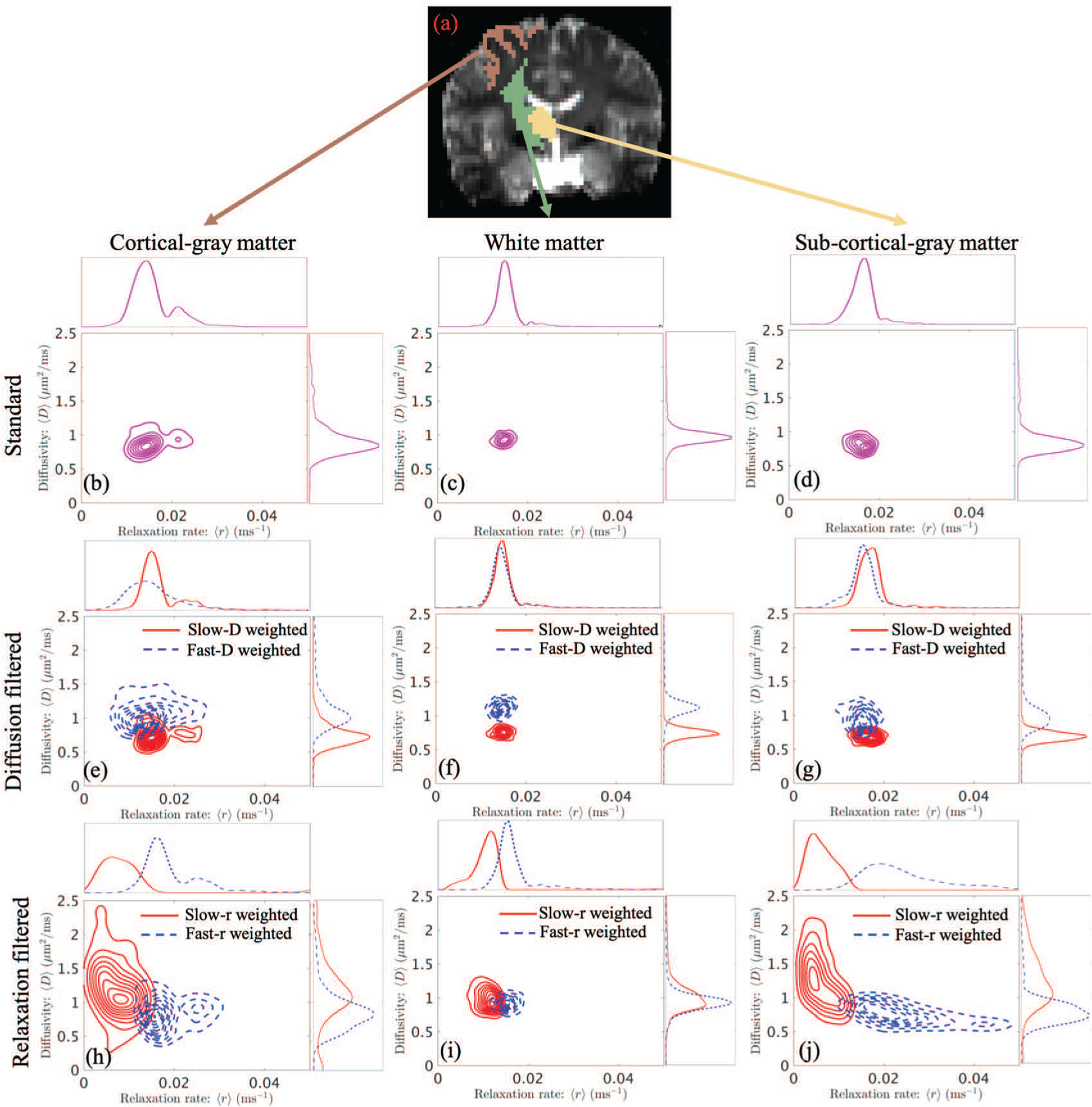
Contour plots of scattered data given by the estimated mean relaxation rate and diffusivity in cortical-gray-matter (left), white-matter (middle) and subcortical-gray-matter (right) regions. The top row illustrates the scattered data of the estimated mean values without using filters. The middle row shows the scattered data given by slow-diffusion and fast-diffusion weighted filters. The bottom row shows results corresponding to slow-relaxation and fast-relaxation weighted filters. It should be noted that the plots reflect the distribution of relaxation and diffusion over multiple voxels rather than the within voxel joint distribution.
The results for filtered PDFs allow us to clearly visualize the heterogeneity of the tissue microstructure in all of the regions. For example, the peak values of the marginal densities corresponding to slow-diffusion and fast-diffusion weighted results clearly separate from each other in all three regions (Figs. (3e), (3f) and (3g)). On the other hand, the marginal densities of relaxation are similar in white matters (Figs. (3f)). The average relaxation of fast-diffusion weighted results is lower than the corresponding results with slow-diffusion weighted filters in cortical and sub-cortical gray matters (the upper plots of Figs. (3e) and (3g)). Moreover, the fast-diffusion filtered relaxation in cortical gray matter (Fig. 3e) has a much higher variance than the other two regions. Furthermore, the slow-diffusion weighted plots in all three regions are similar to the corresponding results in the first row without filters, indicating that the underlying joint PDFs within each voxel may have a dominant mode with relative low diffusivity.
As seen from Figs. (3h), (3i) and (3j), the average diffusivity in all three regions varies significantly with relaxation weighting, indicating high heterogeneity in the tissue composition. For example, for the cortical gray matter region (Fig. (3h)), we observe different relaxation and diffusivity for slow-r and fast-r filters. Similarly, we observe different values for the average relaxation and diffusivities for the filtered PDFs for both white and sub-cortical gray matter regions, which are not observed using the standard technique of estimating the moments (see Figs. (3c) and (3d)). The very similar results in slow-r and fast-r weighted densities in the white-matter region indicates that the underlying tissue components may have similar transverse relaxation rates. It is also interesting to note that the fast-r weighted density in the subcortical-gray-matter in Fig. (3j) spreads over regions close to r = 0.04 ms−1, which is equivalent to a T2 relaxation time of 25 ms. In standard dMRI, the value of TE is relatively long such that the MR signals from tissue components with very fast T2 relaxation rates, such as myelin, are more or less absent. The proposed filtering approach together with the coupling between relaxation and diffusion provide an approach to zoom into tissue components with fast relaxation rates that cannot be probed using current dMRI scans from clinical scanners. It should be noted that though these plots illustrate very different profiles from different brain regions, the precision and accuracy of the estimated results need to be further validated in future work.
C. Comparisons across imaging measures
The first row of Figure 4 shows the mean relaxation rates corresponding to the standard and four types of weighted probability density functions. We observe significant differences between the slow-relaxation (slow-r) and fast-relaxation (fast-r) weighted results indicating heterogeneous relaxation rates at a voxel level in both white and gray matter. Similarly, the relaxation rate seems to be quite different between slow-diffusivity (slow-D) and fast-diffusivity (fast-D) weighted results.
Fig. 4:

The first and second rows illustrate the mean and normalized variance of the relaxation rate corresponding to the standard and the four types of weighted joint probability density functions of relaxation and diffusion.
We note that in Fig. (4b) most cortical-gray matter regions have lower values than white-matter regions, whereas for the fast-r weighted result in Fig. (4c), there is an inverse contrast between the white and gray matter regions, implying that the underlying cortical-gray matter regions have much higher variance than the white matter regions. The slow-diffusivity weighted results show different contrast between cortical-gray matter, white matter and sub cortical gray matter regions. But the fast-D weighted results show similar values in most cortical-gray and white matter regions but much higher values in the subcortical gray matter regions.
The second row in Figure 4 shows the normalized variance of the relaxation rate. As expected, Fig. (2f) shows much higher variance in cortical-gray matter regions than in white matter regions. The higher variance in cortical gray matter regions is also consistently shown in Figs. (2g) to (2j). Moreover, Figs. (2i)) and (2j) are very similar to each other whereas Figs. (2g) and (2f) are significantly different implying that the underlying tissue is potentially more heterogeneous in terms of the relaxation rates.
The three rows of Figure 5 illustrate the average diffusivity (〈D〉), the fractional anisotropy (FA) and the mean kurtosis (MK) as defined earlier in Section 3.2. We note that FA is computed based on dMRI signals at b = 1400 s/mm2. The first column shows the maps for these measures as estimated for the standard joint distribution ρ(r,D). For the slow-r weighted PDF (ρfslow-r), the diffusivity in cortical and subcortical gray-matter regions is much higher than in white-matter regions. But the fast-r weighted maps in the third column show slower diffusivity and higher kurtosis in gray-matter regions, implying that slow-r and fast-r weighted joint PDFs captures information from gray-matter tissue components with significantly different diffusion properties. The slow-r weighted PDF is potentially able to capture information from extra cellular spaces or large cells which act as free water components (and hence the slow relaxation rate), whereas fast-r weighted PDF contains information from intra-axonal or intra-cellular spaces.
Fig. 5:

An illustration of the diffusivity 〈D〉, fractional anisotropy (FA) and mean kurtosis (MK) corresponding to the standard and the four types of weighted joint probability density functions of relaxation and diffusion
The difference between slow- and fast-D weighted results show significant heterogeneity in the underlying diffusion. In particular, the slow-D weighted FA and MK maps are very similar to the standard results except for some voxels with potential partial-volume effects. This implies that the standard joint FA and MK measures are heavily weighted by the slow-D component. The similarity among fast-r and slow-D weighted results indicate that the slow-diffusion components potentially have fast relaxation rates, as expected.
Figure 6 shows the correlation coefficient CDr map between relaxation and diffusion. The results from the different joint PDFs have similar image contrasts in most regions except for some subcortical regions – see the circled regions. In these subcortical regions, the slow-r and fast-r weighted maps have negative and positive correlation, respectively, whereas in the slow-D, fast-D weighted as well as the standard results, the correlation is nearly zero. In all five maps, the cortical gray matter regions have significant negative correlation between diffusivity and relaxation rate.
Fig. 6:
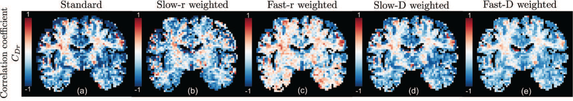
An illustration of the correlation coefficient between relaxation rate and diffusivity for different joint probability density functions.
V. Discussion and conclusions
In this work, we have introduced an approach to use the joint moments of relaxation and diffusion to derive multidimensional imaging measures and to compute relaxation-regressed diffusion signals for estimating fiber orientations. Our approach applied a multiplicative filter to the joint probability density function of relaxation and diffusion to zoom into the statistical properties of the different types of tissue components. We also introduced an expression for the joint moments of the filtered PDFs in terms of the original joint moments of relaxation and diffusion. Theoretically, any type of filter can be applied to select specific diffusion or relaxation bands in the underlying joint distribution. However, for more practical purposes of use in clinical settings and the lack of reliability of the estimated high-order moments from in-vivo clinical data, we introduced four types of linear filters to zoom into tissue components with slow relaxation, fast relaxation, slow diffusion and fast diffusion.
In a proof-of-concept experiment, we applied the proposed method to analyze a dataset acquired from a 3T Siemens Prisma scanner. Experimental results showed that the filtered joint PDFs of relaxation and diffusion had significant differences in their moments, implying heterogeneous components in the underlying tissue. In particular, cortical- and subcortical-gray-matter regions showed much higher variances in relaxation and more significant negative correlation coefficients between relaxation and diffusion than white matter region. The results also revealed different relaxation rates between axonal bundles in complex white matter regions. For the first time, using the proposed relaxation-regressed diffusion signals with different filters, we were able to separate two crossing fiber bundles with different transverse relaxation rates.
The proposed filtering approach can also be applied to analyze other multidimensional imaging data such as diffusion MRI series acquired for different inversion times. In this case, a signal model that uses a finite number of components with different T1 and diffusion tensors has been used to characterize the underlying tissue microstructure [30]. A similar approach was also used in [5] to investigate TE-dependent diffusivity. Moreover, it was shown in [30] that crossing white-matter bundles may have tract-specific T1 values, similar to the results shown in Figs. 1 and 2. However, the performance of this approach depends on the selection of the number of signal components which may vary across brain regions. The proposed approach provides an alternative approach to investigate the coupling of T1 relaxation rate and diffusivity without any dependence on model selection.
A limitation of the proposed method is still the requirement for relatively long scan time. Though the least-squares algorithm is expected to be more reliable than inverse-Laplace transform based methods using fewer number of samples, the in-vivo dataset used in the examples still required 90 minutes of scan time. Our future work will focus on optimizing data acquisition and improving estimation methods in order to reduce scan time and make this approach reliable and practical in clinical settings.
Another limitation of the proposed framework is the assumption of Gaussian diffusion for each component. In particular, the higher-order cumulant moments of diffusivity in Eqs. (2) and (3) are assumed to be only caused by differences in the diffusivity and intra-component non-Gaussian contributions are ignored. Incorporating intra-component non-Gaussianity in the signal representation in Eq. (2) may provide more specific information on tissue microstructure. On the other hand, some recent work have shown that double diffusion encoding sequences are useful to separate micro kurtosis with inhomogeneity in diffusivity [31]. In our future work, we will also explore generalizations of the proposed framework by including micro kurtosis in signal representations and using advanced diffusion encoding sequences.
To summarize, the proposed method has several favorable features. First, the joint moments can be easily estimated compared to the ill-posed estimation of the full joint probability density function. The method is also more robust compared to multi-compartment models, which is plagued by non-unique solutions. Second, the standard non-parametric approach for estimating fiber orientations can be applied to relaxation-regressed diffusion signals to compute the orientation of different fiber components. Third, the imaging measures and fiber orientations from different type of filters could potentially be more sensitive to brain abnormalities than the standard diffusion data acquired at a fixed TE. Therefore, the proposed method provides a new direction to investigate brain structural connections and estimation of their microstructure.
Contributor Information
Lipeng Ning, Brigham and Women’s Hospital, Harvard Medical School, Boston, MA..
Borjan Gagoski, Boston Children’s Hospital, Harvard Medical School, Boston, MA..
References
- [1].Benjamini D and Basser PJ, “Use of marginal distributions constrained optimization (MADCO) for accelerated 2D MRI relaxometry and diffusometry,” Journal of Magnetic Resonance, vol. 271, pp. 40–45, 2016. [DOI] [PMC free article] [PubMed] [Google Scholar]
- [2].Kim D, Doyle EK, Wisnowski JL, Kim JH, and Haldar JP, “Diffusion-relaxation correlation spectroscopic imaging: A multidimensional approach for probing microstructure,” Magnetic Resonance in Medicine, vol. 78, no. 6, pp. 2236–2249, 2017. [DOI] [PMC free article] [PubMed] [Google Scholar]
- [3].Hutter J, Slator PJ, Christiaens D, Teixeira RPA, Roberts T, Jackson L, Price AN, Malik S, and Hajnal JV, “Integrated and efficient diffusion-relaxometry using ZEBRA,” Scientific Reports, vol. 8, no. 1, p. 15138, 2018. [DOI] [PMC free article] [PubMed] [Google Scholar]
- [4].de Almeida Martins JP and Topgaard D, “Multidimensional correlation of nuclear relaxation rates and diffusion tensors for model-free investigations of heterogeneous anisotropic porous materials,” Scientific Reports, vol. 8, no. 2, p. 2488, 2018. [DOI] [PMC free article] [PubMed] [Google Scholar]
- [5].Veraart J, Novikov DS, and Fieremans E, “TE dependent diffusion imaging (TEdDI) distinguishes between compartmental T2 relaxation times,” NeuroImage, vol. 182, pp. 360–369, 2018. [DOI] [PMC free article] [PubMed] [Google Scholar]
- [6].Lampinen B, Szczepankiewicz F, Noven M, van Westen D, Hansson O, Englund E, Martensson J, Westin C-F, and Nilsson M, “Search-˚ ing for the neurite density with diffusion MRI: challenges for biophysical modeling,” arXiv e-prints, p. arXiv:1806.02731, Jun. 2018. [DOI] [PMC free article] [PubMed] [Google Scholar]
- [7].McKinnon ET and Jensen JH, “Measuring intra-axonal T2 in white matter with direction-averaged diffusion MRI,” Magnetic Resonance in Medicine, vol. 0, no. 0, 2018. [DOI] [PMC free article] [PubMed] [Google Scholar]
- [8].Hurlimann M and Venkataramanan L, “Quantitative measurement of¨ two-dimensional distribution functions of diffusion and relaxation in grossly inhomogeneous fields,” Journal of Magnetic Resonance, vol. 157, no. 1, pp. 31–42, 2002. [DOI] [PubMed] [Google Scholar]
- [9].Galvosas P and Callaghan PT, “Multi-dimensional inverse Laplace spectroscopy in the NMR of porous media,” Comptes Rendus Physique, vol. 11, no. 2, pp. 172–180, 2010. [Google Scholar]
- [10].Callaghan P, Godefroy S, and Ryland B, “Use of the second dimension in PGSE NMR studies of porous media,” Magn Reson Imag, vol. 21, pp. 243–248, 2003. [DOI] [PubMed] [Google Scholar]
- [11].Epstein C and Schotland J, “The bad truth about Laplace’s transform,” SIAM Rev, vol. 50, pp. 504–520, 2008. [Google Scholar]
- [12].Bai R, Cloninger A, Czaja W, and Basser PJ, “Efficient 2D MRI relaxometry using compressed sensing,” Journal of Magnetic Resonance, vol. 255, pp. 88–99, 2015. [DOI] [PubMed] [Google Scholar]
- [13].Mitchell J, Chandrasekera T, and Gladden L, “Numerical estimation of relaxation and diffusion distributions in two dimensions,” Progress in Nuclear Magnetic Resonance Spectroscopy, vol. 62, pp. 34–50, 2012. [DOI] [PubMed] [Google Scholar]
- [14].Jian B, Vemuri BC, zarslan E, Carney PR, and Mareci TH, “A novel tensor distribution model for the diffusion-weighted MR signal,” NeuroImage, vol. 37, no. 1, pp. 164–176, 2007. [DOI] [PMC free article] [PubMed] [Google Scholar]
- [15].Scherrer B, Schwartzman A, Taquet M, Prabhu SP, Sahin M, Akhondi-Asl A, and Warfield SK, “Characterizing the distribution of anisotropic micro-structural environments with diffusion-weighted imaging (DIAMOND),” Medical Image Computation and Computer Assisted Intervention (MICCAI), vol. 16, no. 3, pp. 518–526, 2013. [DOI] [PMC free article] [PubMed] [Google Scholar]
- [16].Tuch DS, Reese TG, Wiegell MR, Makris N, Belliveau JW, and Wedeen VJ, “High angular resolution diffusion imaging reveals intravoxel white matter fiber heterogeneity,” Magnetic Resonance in Medicine, vol. 48, no. 4, pp. 577–582, 2002. [DOI] [PubMed] [Google Scholar]
- [17].Assaf Y, Freidlin RZ, Rohde GK, and Basser PJ, “New modeling and experimental framework to characterize hindered and restricted water diffusion in brain white matter,” Magnetic Resonance in Medicine, vol. 52, no. 5, pp. 965–978, 2004. [DOI] [PubMed] [Google Scholar]
- [18].Rathi Y, Gagoski B, Setsompop K, Michailovich O, Grant PE, and Westin CF, “Diffusion propagator estimation from sparse measurements in a tractography framework,” Medical Image Computation and Computer Assisted Intervention (MICCAI), vol. 16, no. 3, pp. 510–517, 2013. [DOI] [PMC free article] [PubMed] [Google Scholar]
- [19].Ning L, Nilsson M, Lasic S, Westin C-F, and Rathi Y, “Cumulantˇ expansions for measuring water exchange using diffusion MRI,” Journal of Chemical Physics, vol. 148, no. 7, p. 074109, 2018. [DOI] [PMC free article] [PubMed] [Google Scholar]
- [20].Veraart J, Poot DHJ, Van Hecke W, Blockx I, Van der Linden A, Verhoye M, and Sijbers J, “More accurate estimation of diffusion tensor parameters using diffusion kurtosis imaging,” Magnetic Resonance in Medicine, vol. 65, no. 1, pp. 138–145, 2011. [DOI] [PubMed] [Google Scholar]
- [21].Jensen JH, Helpern JA, Ramani A, Lu H, and Kaczynski K, “Diffusional kurtosis imaging: The quantification of non-gaussian water diffusion by means of magnetic resonance imaging,” Magnetic Resonance in Medicine, vol. 53, no. 6, pp. 1432–1440, 2005. [DOI] [PubMed] [Google Scholar]
- [22].Andersson JL, Skare S, and Ashburner J, “How to correct susceptibility distortions in spin-echo echo-planar images: application to diffusion tensor imaging,” NeuroImage, vol. 20, no. 2, pp. 870–888, 2003. [DOI] [PubMed] [Google Scholar]
- [23].Andersson JL and Sotiropoulos SN, “An integrated approach to correction for off-resonance effects and subject movement in diffusion MR imaging,” NeuroImage, vol. 125, pp. 1063–1078, 2016. [DOI] [PMC free article] [PubMed] [Google Scholar]
- [24].Avants B, Tustison N, and Gong G, “Advanced normalization tools (ANTS),” Insight J, vol. 2, pp. 1–35, 2009. [Google Scholar]
- [25].Michailovich O, Rathi Y, and Shenton M, “On approximation of orientation distributions by means of spherical ridgelets,” IEEE Trans. Image Process, vol. 19, no. 2, pp. 461–477, 2010. [DOI] [PMC free article] [PubMed] [Google Scholar]
- [26].Basser P, Mattiello J, and LeBihan D, “MR diffusion tensor spectroscopy and imaging,” Biophys J, vol. 66, no. 1, pp. 259–267, 1994. [DOI] [PMC free article] [PubMed] [Google Scholar]
- [27].Gelman N, Gorell J, Barker P, Savage R, Spickler E, Windham J, and Knight R, “MR imaging of human brain at 3.0 T: preliminary report on transverse relaxation rates and relation to estimated iron content.” Radiology, vol. 210, pp. 759–767, 1999. [DOI] [PubMed] [Google Scholar]
- [28].Stanisz GJ, Odrobina EE, Pun J, Escaravage M, Graham SJ, Bronskill MJ, and Henkelman RM, “T1, T2 relaxation and magnetization transfer in tissue at 3T,” Magnetic Resonance in Medicine, vol. 54, no. 3, pp. 507–512, 2005. [DOI] [PubMed] [Google Scholar]
- [29].Lu H, Nagae-Poetscher LM, Golay X, Lin D, Pomper M, and van Zijl PC, “Routine clinical brain MRI sequences for use at 3.0 Tesla,” Journal of Magnetic Resonance Imaging, vol. 22, no. 1, pp. 13–22, 2005. [DOI] [PubMed] [Google Scholar]
- [30].Santis SD, Assaf Y, Jeurissen B, Jones DK, and Roebroeck A, “T1 relaxometry of crossing fibres in the human brain,” NeuroImage, vol. 141, pp. 133–142, 2016. [DOI] [PMC free article] [PubMed] [Google Scholar]
- [31].Paulsen JL, zarslan E, Komlosh ME, Basser PJ, and Song Y-Q, “Detecting compartmental non-Gaussian diffusion with symmetrized double-PFG MRI,” NMR in Biomedicine, vol. 28, no. 11, pp. 1550–1556, 2015. [DOI] [PMC free article] [PubMed] [Google Scholar]