Low-dose megavoltage cone-beam computed tomography using a novel multi-layer imager (MLI)

Abstract

Purpose:

The feasibility of low-dose megavoltage cone-beam acquisition (MVCBCT) using a novel, high detective quantum efficiency (DQE) multi-layer imager (MLI) was investigated. The aim of this work was to reconstruct MVCBCT images using the MLI at different total dose levels, assess Hounsfield Unit (HU) accuracy, noise and CNR for low dose megavoltage cone-beam acquisition.

Methods:

The MLI has four stacked layers; each layer contains a combination of copper filter/converter, gadolinium oxysulfide (GOS) scintillator and a-Si detector array. In total, 720 projections of a CATPHAN® phantom were acquired over 360 degrees at 2.5MV, 6 MV and 6 MV FFF beam energies on a Varian TrueBeam LINAC. The dose per projection was 0.01 MU, 0.0167 MU and 0.05 MU for 2.5 MV, 6 MV and 6 MV FFF respectively. MVCBCT images were reconstructed with varying numbers of projections to provide a range of doses for evaluation. Hounsfield Unit (HU) uniformity, accuracy, noise and CNR were estimated. Improvements were quantified relative to the standard AS1200 single-layer imager.

Results:

Average HU uniformity for the MLI reconstructions was within a range of 95% to 99% for all of the energies studied. Relative electron density estimation from HU values was within 0.4%±1.8% from nominal values. The CNR for MVCBCT based on MLI projections was 2–4x greater than from AS1200 projections. The 2.5 MV beam acquisition with the MLI exhibited the lowest noise and the best balance between CNR and dose for low dose reconstructions.

Conclusions:

MVCBCT imaging with a novel MLI prototype mounted on a clinical linear accelerator was demonstrated the MLI provided substantial improvement over the standard AS1200 EPID. Further optimization of MVCBCT reconstruction, particularly for 2.5 MV acquisitions, will improve image metrics. Overall, the MLI improves CNR at substantially lower doses than currently required by conventional detectors. This new high DQE detector could provide high quality MVCBCT at clinically acceptable doses.

I. INTRODUCTION

The multi-layer imager (MLI) was developed for megavoltage (MV) imaging using layered stacks of detectors to achieve improved performance in detective quantum efficiency (DQE), and noise power spectrum (NPS) [1]. This novel design can benefit task-specific imaging in radiotherapy such as portal imaging, motion-tracking, and MV cone-beam computed tomography (CBCT) by improving image contrast and noise characteristics [2–4]. Previously published work with the MLI included quantitative image metric evaluation on planar images [1, 5], theoretical design optimization studies for MVCBCT [2–4], and feasibility and optimization of MV spectral imaging [6, 7].

Low-dose MVCBCT has been a goal for image-guided radiotherapy [8–15]. However, MVCBCT with conventional electronic portal imagers (EPIDs) suffers from low image contrast as a result of the higher beam energy used to form the image and the limited detection efficiency of the EPID [16]. Coupled with the recent introduction of the 2.5 MV imaging beam line in Varian TrueBeam LINACs, the MLI presents an attractive cost-effective opportunity for achieving improved contrast at clinically acceptable doses.

The scope of the current work was to demonstrate low-dose MVCBCT using a novel, high DQE MLI. The specific objectives of this work were a) to acquire MVCBCT images of a CATPHAN® 604 phantom (CTP604, The Phantom Laboratory, Salem, NY) using clinical 6MV, 6MV flattening filter free (FFF) and 2.5MV beams; b) to compare MVCBCT image quality of MLI acquisitions with that of the standard EPID, and c) to demonstrate high MVCBCT image quality at low dose acquisitions with MLI. This work is the first study of MVCBCT imaging with an MLI prototype mounted on a Varian TrueBeam linear accelerator (LINAC).

II. METHODS

A. MLI and EPID description

The MLI is composed of four stacked imager layers (Fig. 1). Each layer contains a copper/phosphor/detector combination with its own readout amplifier and digitizer. The copper (Cu) component has a thickness of 1 mm. The phosphor is gadolinium oxysulfide (GOS) with 0.436 mm thickness. The detector is an amorphous silicon (aSi) flat-panel array (0.7 mm thickness). The MLI was mounted on a Varian TrueBeam gantry, in place of the conventional EPID. Additional components, such as support layers made of polyethylene are not shown.

Figure 1.

MLI stacked layers and main components. i.e. Copper build-up, GOS phosphor and aSi detector. Corresponding component thickness in mm is also displayed.

The conventional EPID used in this study as the reference imager was the Varian AS1200 model. The AS1200 is composed of a build-up Cu component with the same thickness as MLI (1 mm), a GOS phosphor layer with thickness equal to 0.290 mm (1.5 times less than the GOS phosphor thickness in MLI) and an aSi array.

B. MVCBCT acquisition and phantom

The Varian Truebeam LINAC used for the acquisitions, provided standard 6 MV and 6MV FFF treatment beams, and a 2.5 MV beam (without a flattening filter) specifically designed for imaging. The MLI was attached to the imager arm, replacing the AS1200 EPID within the EPID enclosure. The CATPHAN® 604 phantom was placed on the couch at isocenter. In Table I, the specific inserts used in this study along with corresponding mass and relative electron densities (RED) to water are listed.

Table I.

Sensitometry materials in scan section 2 in CATPHAN 604 (Fig. 2)

Material	Zeff	Density (g/cm3)	Relative electron density to water
Air	8	0.0013	0.001
Teflon	8.43	2.16	1.868
Delrin	6.95	1.42	1.363
Bone 20%	9.09	1.14	1.084
Acrylic	6.47	1.18	1.147
Air	8	0.0013	0.001
Polystyrene	5.7	1.03	0.998
LDPE	5.44	0.92	0.945
Bone 50%	11.46	1.4	1.312
PMP	5.44	0.83	0.853

The Source-Detector Distance (SDD) was 150 cm and the field size at 100 cm (isocenter) was equal to 28×28 cm². The MU per projection was 0.0167 MU at 6 MV, 0.05 MU at 6 MV FFF, and 0.01 at 2.5 MV. In each MVCBCT acquisition, 720 projections were acquired over a full rotation (−180 to 180 degrees). The projections were binned along the Superior-Inferior direction (4 consecutive pixels binned). Due to low MU per pulse at 2.5 MV, four pulses per frame were integrated to achieve quantum-limited acquisitions. Each beam energy was calibrated to provide 1cGy per 1MU at reference conditions. MVCBCT acquisitions were performed with the MLI prototype and the AS1200 single layer EPID as the reference for noise comparison.

The Halcyon™ system, performs MVCBCT using the 6 MV FFF beam and one-layer EPID composed of the same GOS phosphor as a single layer of the MLI (0.436 mm GOS thickness). In clinical MVCBCT acquisitions with Halcyon, the “low dose” scan mode delivers a total of 5 MU over a 200 degree-arc. In the current work, we used the top layer of the MLI to resemble Halcyon acquisitions (henceforth named ‘Halcyon’) to compare performance with all layers of the MLI.

C. Image reconstruction

Projection images were corrected for dark-field (DF), full-field (FF) and defective pixels. MVCBCT images were reconstructed using the Feldkamp-Davis-Kress (FDK) algorithm [17] and iTools Reconstruction v3.0^†. The reconstruction suite provides analytical spectrum correction for beam hardening, ring artifact suppression and asymmetric scatter kernels for scatter correction [18, 19]. At the time of this work, MLI specific scatter kernels had not been implemented in iTools so the scatter correction relied on the AS1200 scatter kernels. This was a reasonable first approximation due to the similar phosphor in each scintillator, respectively.

Subsets of the 720 projections were selected for the following reconstruction schemes: 100, 150, 200, 250, 300, 350, and 400 projections over a 200-degree arc (−90 to 110 degrees). The total MU delivered for each reconstruction are shown in Table II. The image matrix of the reconstructed images was 256×256 pixels per slice and 130 slices along z-direction. The reconstructed image pixel spacing was 1.08×1.08 mm², and the slice thickness was equal to 2 mm.

Table II.

Total MU delivered at each reconstruction

Projections used	Angle span (deg)	MU at 2.5 MV	MU at 6 MV	MU at 6 MV FFF
400	200	4	6.7	20
350	200	3.5		17.5
300	200	3		15
250	200	2.5		12.5
200	200	2	3.3	10
150	200	1.5		7.5
100	200	1	1.7	5

The reconstruction workflow mainly consisted of three stages. In the initial, pre-processing stage, the projections were pre-corrected for various physical effects. Pixel-wise gain and offset differences were first normalized using standard DF and FF calibrations. The projections were then scatter-corrected using a method based on asymmetric kernel superposition [18]. The scatter-corrected projections were then corrected for beam hardening by transforming them to water-equivalent path lengths [20]. The non-linearity expected between the water path length and the attenuation measured by the detector is estimated with analytical calculations using x-ray spectra for each beam and detector efficiency for each pixel from tabulated data. The calculated effect at each pixel is then compensated. In the second stage, the actual reconstruction was performed using the FDK algorithm. Parker weighting was applied for short-scan (200 deg.) reconstructions. In the third stage, various 3D image post-corrections were applied, chiefly ring artifact suppression based on Star-Lack et al, 2010 [19]. Finally, voxel data attenuation values were rescaled to Hounsfield Units. For the mapping from attenuation to HU values, the used slopes were determined to map water to 0 HU. Offset was set to map zero attenuation to −1000 HU.

D. Image metrics

The signal (S) at a specific ROI was estimated as the average HU value within the ROI. The noise (σ) was calculated as the HU standard deviation within the same ROI. The signal inside the ten CATPHAN® material inserts (Fig.2a) was evaluated along with the standard deviation (noise). Background signal for uniformity assessment and noise were assessed in the uniformity section of the CATPHAN® (Fig.2b).

Figure 2.

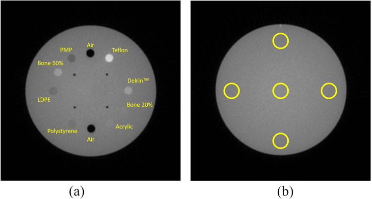
(a) The ten material inserts of the CATPHAN® phantom are labeled. (b) uniformity section of the phantom with associated ROIs represented as yellow circles.

Uniformity estimation was based on Morin et al (2009) [21]:

$$u=\left(1-\frac{\left|S_c-S_p\right|}{S_c-S_{air}}\right)$$ (1)

where S_c is the average HU value on a circular ROI at the center of the central slice, and S_p the average HU value over four circular ROIs at the periphery. S_air is the average HU of air. The average uniformity along the reconstruction schemes of Table II is calculated and Contrast-to-noise ratio (CNR) was estimated at the slice that passes through the center of the inserts at the material inserts section of the CATPHAN® phantom. The CNR was calculated as

$$CN{R}_m=\frac{2\cdot \left|S_m-S_{bgr}\right|}{\sqrt{\left({\sigma }_m^2+{\sigma }_{bgr}^2\right)}}$$ (2)

where $S_{bgr}$ and ${\sigma }_{bgr}$ are the signal and the noise in background, respectively. The subscript, m, refers to the material. The window levels for each figure displayed in the results section was set from −1000 to 1000 HU.

Although, the CATPHAN® 604 contains wire inserts normally used for spatial resolution measurement in kV imaging, these wires were essentially transparent at the MV beam energies studied here. Spatial resolution was therefore quantified instead by fitting Gaussian error functions to the radial edge spread function,

$$\text{ESF}\left(r\right)=a+\frac{b}{2}\left(1+\text{erf}\left(\frac{r-r_0}{\sigma \sqrt{2}}\right)\right)$$ (3)

of an air insert, reconstructed at voxel resolution (0.5 mm³) for the different detector designs. The Full Width at Half Maximum (FWHM) of the corresponding Gaussian point spread function (PSF) was then obtained according to FWHM=2.355σ. For this fitting process, sample voxel values were taken from cylindrical sectors of the air insert, each having an approximate axial length of 16 mm and spanning a 60° arc. Note that phantom tilt with respect to the gantry rotation axis was accounted for in the fit. The process was repeated for different angular positions θ of the sampling area ranging over the 360° perimeter of the insert at 4° intervals. Additionally, for θ=0°, different randomly selected subsets of voxels (10% of the voxels in the sector) were used to perform repeated FWHM calculations and to assess their statistical variability.

III. RESULTS

Figure 3 summarizes the results of the spatial resolution analysis for the different detector configurations. In Fig. 3(a) PSF FWHMs were estimated with sub-voxel variability in all cases. The median PSF widths showed sub-voxel variability across the different detector configurations. Figure 3(b) plots the variation in measured PSF width around the perimeter of the insert.

Figure 3.

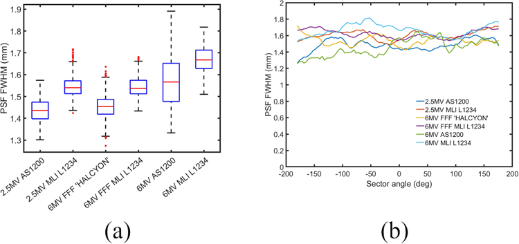
(a) Box-plot showing distribution of PSF width calculations for θ=0° (b) The computed PSF widths at different sector angles θ ranging from −180° to 180°.

Table III contains HU uniformity results for AS1200 at 2.5 MV and 6 MV, MLI at 2.5 MV, 6MV, and 6 MV FFF reconstructions, calculated using (1). The results are averaged per beam energy over all reconstruction schemes detailed in Table II. There are very small deviations in u between different reconstructions of the same energy. Uniform HU were maintained along the center and the periphery of the phantom. This is partially expected as the different reconstructions are obtained from various subsets of the same scan.

Table III.

MLI HU uniformity averaged over different reconstructions (Table II) at each beam energy

	2.5 MV AS1200	6 MV AS1200	2.5 MV MLI L1234	6 MV MLI L1234	6 MV FFF MLI L1234
u	0.986±5.3×10−4	0.990±2.3×10−3	0.994 ± 2.4×10−4	0.997 ± 1.0×10−3	0.995 ± 4.2×10−4

Reconstructed images of the AS1200 and MLI with all layers combined (L1234) were compared at total delivered dose of 2 MU for 2.5 MV beam energy (Fig. 4). The AS1200 image is noisier with prominent artifacts in the central part of the reconstructed image (Fig.4a). These are likely caused by detector non-linearities at low counts during 2.5 MV beam acquisition. Images reconstructed with MLI top layer (‘Halcyon’) and MLI all layers (MLI L1234) for a 5 MU, 6MV FFF acquisition, are shown in Fig 5. The image of the MLI L1234 is less noisy due to the increased number of layers used. Coronal views, reconstructed with 0.5 mm slice thickness, were also included in Fig. 4c–d, and Fig. 5c–d to qualitatively demonstrate the difference in image quality between AS1200, ‘HALCYON’ and MLI. Similar image quality difference was observed on sagittal views.

Figure 4.

Reconstructed material inserts slices for (a) AS1200 and (b) MLI with all layers combined at 2.5MV beam acquisitions and similar delivered MU. The corresponding Coronal views are shown in (c) and (d) respectively at 0.5 mm reconstructed slice thickness.

Figure 5.

Reconstructed material inserts slices for (a) MLI top layer ‘Halcyon’ and (b) MLI with all layers combined at 6MV FFF beam acquisitions and similar delivered MU. The corresponding Coronal views are shown in (c) and (d) respectively at 0.5 mm reconstructed slice thickness.

Relative electron density (RED) was a linear function of HU for each beam mode used. Nominal versus estimated RED is shown in Fig. 6. There is generally very good agreement between expected and measured RED. In Table IV, the comparison of estimated RED and nominal RED values for the material inserts is shown. In general, the RED was estimated within 0.4% ± 1.8% of the corresponding nominal values. Estimation of the LDPE insert had the largest disagreement with the nominal values of RED (3.4%).

Figure 6.

Measured against expected relative electron density for (a) 2.5 MV, (b) 6 MV FFF, and (c) 6 MV reconstructions using 400 projections over a 200-degree acquisition. Error bars were too small to display.

Table IV.

Comparison between nominal and estimated RED values from HU of the reconstructed material inserts slice. Percentage difference is shown inside the parentheses.

Material	Nominal RED	Estimated RED 2.5 MV	Estimated RED 6MV MV	Estimated RED 6 MV FFF
Teflon	1.868	1.874 (0.3%)	1.858 (−0.5%)	1.858 (−0.6%)
Delrin	1.363	1.343 (−1.5%)	1.324 (−2.9%)	1.355 (−0.6%)
Bone20	1.084	1.111 (2.5%)	1.094 (0.9%)	1.112 (2.6%)
Acrylic	1.147	1.133 (−1.2%)	1.139 (−0.7%)	1.132 (−1.3%)
Polystyrene	0.998	0.993 (−0.5%)	1.012 (1.4%)	0.994 (−0.4%)
LDPE	0.945	0.944 (−0.1%)	0.977 (3.4%)	0.946 (0.1%)
Bone50	1.312	1.321 (0.7%)	1.329 (1.3%)	1.330 (1.3%)
PMP	0.853	0.848 (−0.6%)	0.853 (0.1%)	0.848 (−0.6%)

Background noise in HU is shown in Fig. 7 for 2.5 MV, 6 MV and 6 MV FFF reconstructions with the MLI. The HU noise for the AS1200 acquisition of 2.5 MV projections (blue line), 6MV projections (gray line) and ‘Halcyon’ 6MV FFF (yellow line) are also shown as reference. The 2.5 MV beam reconstructions demonstrated better noise performance at low MU (i.e. low dose).

Figure 7.

Noise (standard deviation of HU values) for different beam energies with ‘Halcyon’, MLI, and AS1200 at 2.5MV, 6MV and 6MV FFF.

Relative CNR improvement between MLI and AS1200 at 2.5 MV beam energy, and MLI and ‘Halcyon’ at 6 MV FFF beam energy respectively is tabulated in Tables V and VI. The corresponding relative CNR for each material insert is shown. The CNR of images reconstructed from MLI projections compared to AS1200 increased by a factor approximately between 2 and 4 depending on material (Table V) and up to 2 when compared with ‘Halcyon’ reconstructed images at 6 MV FFF. Absolute CNR plots versus MU for the 50% Bone and LDPE (low-density polyethylene) are shown in Fig. 8 and 9, respectively, for 2.5MV, 6MV FFF and 6MV beams.

Table V.

Relative CNR improvement of MLI over AS1200 at 2.5 MV beam energy.

MU	Air	Teflon	Delrin	Bone 20%	Bone 50%	Acrylic	Polystyrene	LDPE	PMP
4	3.9	4.2	2.9	2.2	2.7	2.2	2.8	2.1	2.6
3.5	3.9	4.1	2.8	2.1	2.6	2.1	2.8	2.1	2.5
3	3.8	4.1	2.8	2.1	2.6	2.0	2.7	2.1	2.5
2.5	3.8	3.9	2.7	2.2	2.5	2.0	2.7	2.2	2.3
2	3.7	3.8	2.7	2.0	2.4	2.0	2.8	2.1	2.5
1.5	3.6	3.6	2.7	2.0	2.2	2.2	2.5	2.1	2.3
1	3.4	3.3	2.6	2.0	2.2	2.0	2.6	1.9	2.1

Table VI.

Relative CNR improvement of MLI over ‘HALCYON’ at 6 MV FFF beam energy.

MU	Air	Teflon	Delrin	Bone 20%	Bone 50%	Acrylic	Polystyrene	LDPE	PMP
20	1.1	1.3	1.7	1.6	1.7	1.9	1.9	1.6	1.7
17.5	1.2	1.3	1.7	1.6	1.8	1.8	1.9	1.6	1.7
15	1.2	1.4	1.7	1.7	1.8	1.9	1.9	1.6	1.7
12.5	1.2	1.4	1.7	1.6	1.7	1.9	1.9	1.7	1.8
10	1.3	1.4	1.8	1.7	1.8	1.8	1.9	1.7	1.8
7.5	1.3	1.4	1.7	1.6	1.8	1.9	1.8	1.7	1.8
5	1.4	1.5	1.7	1.6	1.8	1.8	2.0	1.8	1.8

Figure 8.

CNR for the 50% bone insert, for different beam energies with ‘Halcyon’, MLI, and AS1200 at 2.5MV, 6MV and 6MV FFF.

Figure 9.

CNR for LDPE insert, for different beam energies with ‘Halcyon’, MLI, and AS1200 at 2.5MV, 6MV and 6MV FFF. The y-axis scale is different from that in Fig. 7.

IV. DISCUSSION

The stacked format of the MLI increases x-ray detection efficiency without the loss of resolution associated with thick scintillator detectors [2]. In the current work, we address the potential for low-dose, high-image-quality MVCBCT acquisition with the MLI. Based on the MLI construction, we expected to achieve improved image quality performance compared to AS1200 EPID at low dose. This can be qualitatively observed in the reconstructions in Fig. 3 and 4.

The reconstruction process included scatter and beam hardening corrections that depend on various acquisition properties (such as beam spectrum, spectral sensitivity of the imaging device, filtering properties and scintillation scatter). Since the MLI design is under active development, a detailed description of the properties required for optimum reconstruction has not yet been completed. MVCBCT reconstructions with the MLI were performed using the available properties and reconstruction data for the AS1200. Hence, some cupping artifacts were not optimally corrected for the MLI. In general, the reconstruction included a scatter correction step to compensate for scatter generated in the object. Beam-hardening is compensated assuming water and using the beam and detector efficiency spectrum. Therefore, the same kernels were used for both imaging devices (MLI and AS1200), resulting in, sub-optimal scatter correction for the MLI imager. It is anticipated that optimization of the reconstruction can further improve the MLI MVCBCT reconstructed images.

In Fig. 3(a), the median PSF widths showed sub-voxel variability across the different detector configurations. A slight degradation in spatial resolution was observed in each multi-layer configuration as compared to its single layer counterpart but was too small to have a perceptible impact visually. Figure 3(b) indicates nearly uniform edge blur. Because FDK reconstruction (as opposed to iterative model-based reconstruction) was used throughout our work, strongly non-uniform spatial resolution would be expected only if significant detector lag, which was not corrected for in our imaging chain, were present. The trends in Fig. 3(b) give evidence that this was not the case.

Estimated electron density displayed a nearly one-to-one correspondence to nominal electron density for all beam energies (Fig.6). The MLI provides an approximately twofold noise improvement compared with the standard AS1200 EPID (Fig. 7). Relative CNR Tables V and VI, and Figures 7–9 clearly demonstrate that the 2.5 MV beam combined with the MLI has the best overall MVCBCT imaging performance at low dose delivery. Interestingly, reconstructions at low-MU with ‘Halcyon’ (5 MU), show worse or similar noise performance with AS1200 low-dose (2 MU) reconstructions at 2.5 MV beam (Fig. 7). This can also be observed qualitatively in Fig. 4(a) and Fig 5(a). Higher noise in Halcyon can be attributed to a) lower absorption of higher energy x-rays at the scintillator, and b) the number of projections used to reconstruct the Halcyon image at 5 MU is half those used for the AS1200 image at 2MU (100 vs 200 projections respectively).

In Fig. 8 and 9, results for 2.5 MV, 6MV, and 6MV FFF beam energies are also shown. The 2.5 MV reconstruction with AS1200 demonstrates better performance in the low-density material than the 6 MV reconstruction with the MLI (Fig. 9). This can be largely attributed to the higher content of low-energy x-rays in the 2.5 MV that are absorbed in the scintillator and contribute to lower noise and improved contrast for low-density materials. However, for Varian LINACs, the 6 MV FFF or the 2.5 MV beams are more likely to be used for MV imaging.

MU was used as a surrogate for dose under the assumption of standard calibration (1 MU = 1 cGy at reference conditions). Dose measurements for MVCBCT using indices directly comparable with kVCBCT, such CTDI or CBDI were not performed. These metrics would have a different meaning with MV beams and are not easily translatable between kV and MV. The 3D distribution of dose is markedly different in MV beams, even at low imaging doses, compared with kV. In the future, a different metric for evaluating MV-CBCT dose may be developed. In the meantime, MU is a reasonable method for inter-comparison of MV-CBCT protocols.

Low-dose MVCBCT acquisitions in a Truebeam LINAC are not clinically available at this time. The acquisitions described in this work were performed at Varian’s Imaging Laboratory (iLAB) in Baden, Switzerland under non-clinical experimental conditions. This limited the dose parameter space in our investigation. Future developments in the pulse generation hardware could enable low-dose clinical image acquisition.

Adaptive radiotherapy is a potential application of MVCBCT which could be supported by the MLI. On-line replanning requires accurate electron density of the imaged tissue. Since this is obtained from CT images using a HU to electron density conversion, adaptive planning requires a high accuracy of HU to electron density conversion. We found this to be achievable for MVCBCT with the MLI, particularly in tissues with inhomogeneities. Table IV demonstrated very good agreement between estimated and nominal relative electron densities. Dosimetric evaluation of HU to RED conversion was out of the scope of the current work but will be assessed in future studies.

V. CONCLUSION

The feasibility of low-dose MVCBCT imaging using a novel MLI prototype mounted on a Varian TrueBeam LINAC was demonstrated at various delivered dose levels. Investigation of the reconstructed image quality and total delivered dose demonstrated major improvements in CNR with the MLI compared with a conventional AS1200 EPID. In addition, using the 2.5 MV beam further reduces the imaging dose needed for high CNR, compared to 6 MV and 6 MV-FFF, while maintaining high HU accuracy. Acquisition of high-quality MV-CBCT images with doses as low as 1 MU opens up the potential for clinical translation. Impacted applications include metal artifact reduction and dose calculation for adaptive radiotherapy.

References

- 1.Rottmann J, Morf D, Fueglistaller R, Zentai G, Star-Lack J, and Berbeco R, A novel EPID design for enhanced contrast and detective quantum efficiency, Phys. Med. Biol 61(17), 6297–6306 (2016). [DOI] [PMC free article] [PubMed] [Google Scholar]
- 2.Hu Y-H, Myronakis M, Rottmann J, et al. , A novel method for quantification of beam’s-eye-view tumor tracking performance, Med. Phys 44(11), 5650–5659 (2017). [DOI] [PMC free article] [PubMed] [Google Scholar]
- 3.Hu Y-H, Rottmann J, Fueglistaller R, et al. , Leveraging multi-layer imager detector design to improve low-dose performance for megavoltage cone-beam computed tomography, Phys. Med. Biol 63(3), 035022 (2018). [DOI] [PMC free article] [PubMed] [Google Scholar]
- 4.Hu Y-H, Fueglistaller R, Myronakis ME, et al. , Physics considerations in MV-CBCT multi-layer imager design, Phys. Med. Biol (2018). [DOI] [PMC free article] [PubMed]
- 5.Myronakis M, Star-Lack J, Baturin P, et al. , A novel multi-layer MV imager computational model for component optimization, Med. Phys (2017). [DOI] [PMC free article] [PubMed]
- 6.Myronakis ME, Fueglistaller R, Rottmann J, et al. , Spectral imaging using clinical megavoltage beams and a novel multi-layer imager, Phys. Med. Biol 62(23), 9127–9139 (2017). [DOI] [PMC free article] [PubMed] [Google Scholar]
- 7.Myronakis M, Hu Y-H, Fueglistaller R, et al. , Multi-layer imager design for mega-voltage spectral imaging, Phys. Med. Biol 63(10), 105002 (2018). [DOI] [PMC free article] [PubMed] [Google Scholar]
- 8.Pouliot J, Bani-Hashemi A, Chen Josephine, et al. , Low-dose megavoltage cone-beam CT for radiation therapy, Int. J. Radiat. Oncol 61(2), 552–560 (2005). [DOI] [PubMed] [Google Scholar]
- 9.Pouliot J, Megavoltage Imaging, Megavoltage Cone Beam CT and Dose-Guided Radiation Therapy, in IMRT, IGRT, SBRT - Adv. Treat. Plan. Deliv. Radiother(KARGER, Basel, 2007), pp. 132–142. [DOI] [PubMed] [Google Scholar]
- 10.Morin O, Gillis A, Descovich M, et al. , Patient dose considerations for routine megavoltage cone-beam CT imaging, Med. Phys 34(5), 1819–1827 (2007). [DOI] [PubMed] [Google Scholar]
- 11.Faddegon BA, Wu V, Pouliot J, Gangadharan B, and Bani-Hashemi A, Low dose megavoltage cone beam computed tomography with an unflattened 4 MV beam from a carbon target, Med. Phys 35(12), 5777–5786 (2008). [DOI] [PubMed] [Google Scholar]
- 12.Breitbach EK, Maltz JS, Gangadharan B, et al. , Image quality improvement in megavoltage cone beam CT using an imaging beam line and a sintered pixelated array system, Med. Phys 38(11), 5969–5979 (2011). [DOI] [PubMed] [Google Scholar]
- 13.Fast MF, Koenig T, Oelfke U, and Nill S, Performance characteristics of a novel megavoltage cone-beam-computed tomography device, Phys. Med. Biol 57(3), N15–N24 (2012). [DOI] [PubMed] [Google Scholar]
- 14.Liu L, Antonuk LE, El-Mohri Y, Zhao Q, and Jiang H, Optimization of the design of thick, segmented scintillators for megavoltage cone-beam CT using a novel, hybrid modeling technique, Med. Phys 41(6Part1), 061916 (2014). [DOI] [PMC free article] [PubMed] [Google Scholar]
- 15.Tang G, Moussot C, Morf D, Seppi E, and Amols H, Low-dose 2.5 MV cone-beam computed tomography with thick CsI flat-panel imager, J. Appl. Clin. Med. Phys 17(4), 235–245 (2016). [DOI] [PMC free article] [PubMed] [Google Scholar]
- 16.Antonuk LE, Electronic portal imaging devices: a review and historical perspective of contemporary technologies and research., Phys. Med. Biol 47(6), R31–65 (2002). [PubMed] [Google Scholar]
- 17.Feldkamp LA, Davis LC, and Kress JW, Practical cone-beam algorithm, J. Opt. Soc. Am. A 1(6), 612 (1984). [Google Scholar]
- 18.Sun M and Star-Lack JM, Improved scatter correction using adaptive scatter kernel superposition, Phys. Med. Biol 55(22), 6695–6720 (2010). [DOI] [PubMed] [Google Scholar]
- 19.Star-Lack J, Mostafavi H, Pavkovich J, inventors; Varian Medical Systems Inc, assignee. System and method for correcting for ring artifacts in an image. United States patent US 7,860,341. 2010. December 28.
- 20.Joseph P and Spital R, A Method for Correcting Bone Induced Artifacts in Computed Tomography Scanners, J. Comput. Assist. Tomogr 2(1), 100–108 (1978). [DOI] [PubMed] [Google Scholar]
- 21.Morin O, Aubry J-F, Aubin M, et al. , Physical performance and image optimization of megavoltage cone-beam CT, Med. Phys 36(4), 1421–1432 (2009). [DOI] [PubMed] [Google Scholar]