Rapid Dealiasing of Undersampled, Non-Cartesian Cardiac Perfusion Images using U-Net

Abstract

Compressed sensing (CS) is a promising method for accelerating cardiac perfusion MRI to achieve clinically acceptable image quality with high spatial resolution (1.6×1.6×8mm³) and extensive myocardial coverage (6–8 slices per heartbeat). A major disadvantage of CS is its relatively lengthy processing time (~8 min per slice with 64 frames using GPU), thereby making it impractical for clinical translation. The purpose of this study was to implement and test whether an image reconstruction pipeline including a neural network is capable of reconstructing 6.4-fold accelerated, non-Cartesian(radial) cardiac perfusion k-space data at least 10 times faster than CS, without significant loss in image quality. We implemented a 3D (2D+time) U-Net and trained it with 132 2D+time datasets (coil-combined, zero-filled as input; CS reconstruction as reference) with 64 time frames from 28 patients (8448 2D images in total). For testing, we used 56 2D+time coil-combined, zero-filled datasets (3584 2D images in total) from 12 different patients as input to our trained U-Net, and compared the resulting images with CS reconstructed images using quantitative metrics of image quality and visual scores (conspicuity of wall enhancement, noise, artifacts; each score ranging from 1[worst] to 5[best], with 3 defined as clinically acceptable) evaluated by readers. Including pre- and post-processing steps, compared with CS, U-Net significantly reduced the reconstruction time by 14.4 times (32.1±1.4s for U-Net vs. 461.3±16.9s for CS, p<0.001), while maintaining high data fidelity (structural similarity index =0.914±0.023, normalized root mean square error=1.7±0.3%, identical mean edge sharpness of 1.2 mm). The median visual summed score was not significantly different (p=0.053) between CS (14; interquartile range [IQR]=0.5) and U-Net (12; IQR=0.5). This study shows that the proposed pipeline with a U-Net is capable of reconstructing 6.4-fold accelerated, non-Cartesian cardiac perfusion k-space data 14.4 times faster than CS, without significant loss in data fidelity or image quality.

Graphical Abstract

This study describes implementation of an image reconstruction pipeline including a U-Net architecture for reconstructing 6.4-fold accelerated, non-Cartesian cardiac perfusion MRI k-space data at least 10 times faster than a GPU-accelerated compressed sensing (CS) reconstruction pipeline, without significant loss in data fidelity or image quality. Our U-Net was trained on 132 2D+time datasets (zero-filled as input, CS reconstruction as output) from 28 patients. Testing of our U-Net in 12 patients show the following results. Compared with CS, U-Net significantly reduced the reconstruction time by 14.4 times (32.1 ± 1.4 s for U-Net vs. 461.3 ± 16.9 s for CS, p<0.001), while maintaining high data fidelity (structural similarity index = 0.914 ± 0.023, normalized root mean square error = 1.7 ± 0.3%, identical mean edge sharpness of 1.2 mm). The median visual summed score was not significantly (p = 0.053) different between CS (14; interquartile range = 0.5) and U-Net (12; interquartile range = 0.5). This study shows that the proposed pipeline with a U-Net is capable of reconstructing 6.4-fold accelerated, non-Cartesian cardiac perfusion k-space data 14.4 times faster than CS, in less than 1 min per slice with 64 frames, without significant loss in data fidelity or image quality.

Introduction

Coronary artery disease (CAD) is a leading cause of death and sickness in the United States¹. First-pass myocardial perfusion MRI is as accurate as cardiac SPECT for detecting CAD². One area of active research is improving myocardial coverage with accelerated multi-slice 2D imaging^3–7 or 3D imaging^8–10, for the purpose of achieving volumetric coverage like SPECT. To date, multi-slice 2D imaging is more common in practice because it lends itself to sampling throughout the cardiac cycle, whereas for 3D imaging only a fraction of the cardiac cycle is sampled to account for cardiac and respiratory motion.

Compressed sensing (CS)¹¹ is a promising method for accelerating cardiovascular MRI. It provides a means to accelerate beyond parallel imaging methods such as k-t BLAST or k-t SENSE¹², but at the expense of computational efficiency. We have recently developed a 6.4-fold accelerated 2D cardiac perfusion MRI pulse sequence using radial k-space sampling and compressed sensing (CS)¹¹ to achieve clinically acceptable image quality with high spatial resolution (1.6 mm × 1.6 mm × 8 mm) and extensive myocardial coverage (6–8 2D slices per heartbeat, depending on heart rate)⁶. While CS is a promising method from an imaging perspective, its relatively lengthy image reconstruction (e.g. ~8 min per slice with 64 frames using GPU) makes it impractical for clinical translation. Thus, a faster image reconstruction pipeline is necessary for clinical translation of the aforementioned pulse sequence.

This study focuses on deep learning (DL) as a means to highly accelerate the image reconstruction pipeline¹³. The advantage of DL over CS is that the processing speed is considerably faster, because once a neural network is trained its processing during testing is not iterative. While there are many implementations of neural networks for MR image reconstruction, we focused on two studies that demonstrated successful implementation of 3D neural networks for 2D cardiac cine MRI. One proof-of-concept DL study used a cascade of 3D convolutional neural networks (CNNs)¹⁴ to reconstruct undersampled Cartesian k-space data while including a data consistency layer. This study, however, did not evaluate the performance on non-Cartesian k-space data. Another proof-of-concept DL study used a 3D residual U-Net¹⁵ to dealiase zero-filled images derived from undersampled non-Cartesian k-space data, but without a data consistency layer. Neither studies investigated the performance of their networks on dynamic contrast-enhanced cardiac perfusion MRI with time-varying signal and low signal-to-noise ratio. For practical reasons, we elected against neural networks including either a data consistency layer or k-space terms, in order to work within the memory limit of our GPU computer and avoid computationally intensive nonuniform fast Fourier transform (NUFFT) for translating data between Cartesian and polar coordinates. As such, we elected to adapt the U-Net proposed by Hauptmann et al.¹⁵ to rapidly dealiase 2D undersampled, non-Cartesian cardiac perfusion images without a data consistency layer. In this study, we sought to implement an image reconstruction pipeline including a 3D residual U-Net and test whether it is capable of reconstructing undersampled, non-Cartesian 2D cardiac perfusion k-space data at least 10 times faster than GPU-accelerated CS reconstruction, in less than 1 min per slice with 64 frames, without significant loss in data fidelity or image quality.

Methods

Patients

We prospectively enrolled 27 patients (20 men and 7 women, mean age = 55 ± 15 years) undergoing a clinical cardiovascular MRI with administration of gadolinium-based contrast agent for assessment of myocardial infiltration or viability. As these clinical MRI scans did not involve a dynamic contrast-enhanced MRI, they provided us an opportunity to add resting perfusion scans for research without significantly altering the clinical MRI protocol. To expand the database, we combined those k-space datasets to a pool of existing perfusion k-space data of 13 patients (8 men and 5 women, mean age = 43 ± 12 years) obtained from a prior study⁶. Combining both k-space data sets is justifiable since they were acquired using an identical pulse sequence in patients with similar clinical indications. We randomly split 40 patients as the following: 28 for training, and 12 for testing. All subjects provided written informed consent. This study was performed in accordance with protocols approved by our institutional review board and was Health Insurance Portability and Accountability Act (HIPAA) compliant. See Supporting Table S1 in Supplementary Materials for basic clinical profiles of our patient population.

MRI Hardware

MRI was performed on two 1.5T whole-body MRI scanners (MAGNETOM Aera and Avanto, Siemens Healthineers, Erlangen, Germany) equipped with a gradient system capable of achieving a maximum gradient strength of 45 mT/m and a slew rate of 200 T/m/s. In this study, 30 and 10 patients were scanned on the Avanto and Aera scanner, respectively. MRI signal reception was made using anterior and posterior coil arrays with 15 and 30 total coil elements on the Avanto and Aera, respectively.

Pulse Sequence

Relevant imaging parameters for our 2D multi-slice cardiac perfusion pulse sequence using gradient echo readout with radial k-space sampling included: field of view (FOV) = 300 mm × 300 mm, acquisition matrix = 192 × 192, spatial resolution = 1.6 mm × 1.6 mm, slice thickness = 8 mm, TE/TR = 1.5/2.6 ms, flip angle = 12°, receiver bandwidth = 700 Hz/pixel, 30 rays per frame with the 7^th Fibonacci sequence of golden angles (=23.628°)¹⁶, single-shot readout duration per frame = 78 ms, 75 repetitions, electrocardiogram triggering every heartbeat, and 6–8 slices per heartbeat, depending on heart rate. Each patient was instructed to breathe normally during scanning. For more details on the pulse sequence, please see reference⁶.

Each perfusion scan was performed with administration of 0.1 mmol/kg of gadobutrol (Gadavist, Bayer HealthCare Whippany, USA) at 4–5 mL/s via a power injector. Gadobutrol was diluted with equal volume of saline, and this mixture was administered via an antecubital IV injection followed by a 20 mL of saline flush.

Image Reconstruction

GPU-Accelerated CS Reconstruction as Practical Ground Truth

In dynamic contrast-enhanced cardiac perfusion MRI, it is difficult to obtain fully sampled, single-shot datasets without incurring motion artifacts. In this study, we used CS-accelerated cardiac perfusion MRI datasets as practical ground truths. Our original CS reconstruction implemented on a CPU, excluding motion correction, on average required 163 min to reconstruct each perfusion slice with 75 temporal frames⁶. For this study, we implemented a GPU-accelerated CS reconstruction pipeline on the same GPU hardware as our U-Net, in order to reduce the CS reconstruction time from 163 min to approximately 8 min per slice with 64 frames, as well as conduct a fair comparison in computation efficiency by using the same GPU hardware as deep learning. In addition, only the first 64 frames were reconstructed with CS to match the 64 frames reconstructed using U-Net with 2 × 2 × 2 maxpooling. During post-processing, residual aliasing artifacts were filtered using block-wise low rank (BWLR) with a single iteration, as previously described⁶. Relevant parameters for BWLR included: image block size = 8 × 8 and normalization threshold value = 20% of the absolute maximum value. For convenience, unless otherwise stated, we refer CS plus BWLR filtering as CS throughout.

Imaging Reconstruction Pipeline including Pre-Processing, U-Net, and Post-Processing Steps

Our proposed image reconstruction pipeline includes three sequential steps: In step 1 (pre-processing), the radial k-space data were gridded and transformed into zero-filled images in Cartesian space using GPU-accelerated NUFFT¹⁷, followed by weighted sum over the coil elements. In step 2 (dealiasing), the trained U-Net was used to dealiase coil-combined, zero-filled image. In step 3, residual aliasing artifacts were filtered using BWLR with a single iteration with image block size = 8 × 8 and normalization threshold value = 10% of the absolute maximum value.

U-Net Training and Testing

We implemented a 3D residual U-Net architecture¹⁵ (see Figure 1) on a GPU workstation (P100 Tesla 12 GB memory, NVIDIA, Santa Carla, California, USA; Xeon E5–2650 v4 128 GB memory, Intel, Santa Clara, California, USA) equipped with Python (Version 3.6, Python Software Foundation) and TensorFlow running on a Linux operation system (Ubuntu16.04). Relevant details of our 3D U-Net architecture included: 3 layers, 16 features, mini-batch size =4, Adam optimizer, 10,000 iterations or 10,000/33 epochs, learning rate= 0.025, which decreased by 90% each 500 iterations, 3 × 3 × 3 convolutional kernel, and 2 × 2 × 2 pooling size. These settings were fined tuned based on visual inspection on training data. We considered a U-Net with 4 layers and 32 features but decided against it when we discovered that it did not significantly improve results over a network with 3 layers and 16 features (see Supporting Figure S1 in Supplementary Materials).

Figure 1.

A schematic architecture of residual 3D U-Net. The number above each block corresponds to the number of features for each layer. The number in the left of each block corresponds to the matrix size at every level. Each convolutional layer has a 3 × 3 × 3 kernel and a rectified linear unit, except for the last layer that produced the residual update. Between different layers, a 2 × 2 × 2 max pooling size was used.

As shown in Figure 2, for training, we used 132 2D+time datasets with 64 frames per slice (or 8448 2D images in total) from 28 randomly selected patients, where the coil-combined, zero-filled images were used as input and the corresponding CS reconstructed images without BWLR filtering were used as output. We grouped all temporal frames per slice because that represents a unit for perfusion analysis, and then concatenated multiple time series as batches. Our network was trained by minimizing the l₂-loss of the reconstructed images to the CS images in an iterative manner, as previously described^18–20. Our U-Net required 11 hours and 53 min to train. For testing, we used 56 2D+time datasets with 64 frames per slice (i.e. 3584 2D images in total) from 12 remaining patients as input to our trained U-Net, and the resulting images were compared with CS reconstructed images with BWLR filtering. For cross validation, we randomly selected 12 patients from the training side and swapped them with the testing patients, and repeated the process of training and testing as described above.

Figure 2.

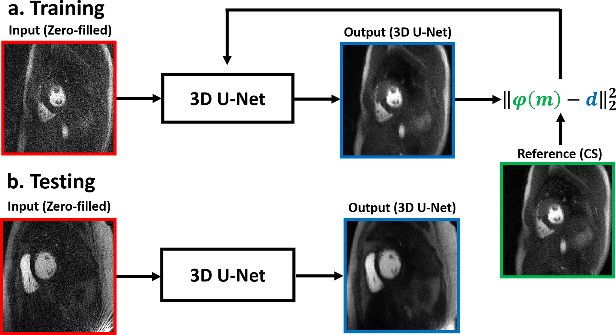
Schematics illustrating the training and testing steps. (a) For training, we used 132 2D+time datasets with 64 frames per slice (or 8448 2D images in total) from 28 randomly selected patients, where the coil-combined, zero-filled images were used as input and the corresponding CS reconstructed images without BWLR filtering were used as output. Our network was trained by minimizing the l₂-loss of the reconstructed images to the CS images. (b) For testing, we used 56 2D+time datasets with 64 frames per slice (i.e. 3584 2D images in total) from 12 remaining patients as input to our trained U-Net.

We considered having our U-Net learn both CS and BWLR filtering, but discovered that our network learned CS without BWLR better than both combined with our limited training data (see Supporting Figure S2 in Supplementary Materials). Thus, we applied BWLR during post-processing (step 3), immediately after dealising with U-Net (step 2). For convenience, unless otherwise stated, we refer U-Net plus BWLR filtering as U-Net throughout.

Quantitative Metrics of Image Quality

Given that CS and U-Net images are perfectly registered, we calculated the structural similarity index (SSIM)²¹ and normalized root mean square error (NRMSE) to infer data fidelity with CS as the reference. For both SSIM and NRMSE calculations, we limited the analysis to the heart region by manually cropping the FOV, as shown in Figure 3. For evaluation of image blurring, we measured an intensity profile through the left ventricular cavity and myocardial wall at peak blood enhancement and calculated the distance between the 25 and 75 percentiles of peak intensity value. To increase precision in calculating the edge profiles, we interpolated each intensity profile by a factor of 20 using a spline curve fitting routine (see Figure 3).

Figure 3:

(Left) A smaller region-of-interest was used to calculate SSIM and NRMSE. (Right) Edge sharpness was calculated across the left ventricular cavity and myocardial wall (green lines) at the peak blood enhancement, defined as the distance between 25th and 75th percentiles (blue dotted lines) of peak intensity values for a given profile.

Visual Scores of Image Quality

Seventy-two rest perfusion datasets (3 short-axis planes from each of 12 patients, multiplied by 2 reconstruction types) were randomized and de-identified for independent evaluation by 2 readers using a 5-point Likert scale for the following three categories: conspicuity of wall enhancement (1: nondiagnostic; 2: poor; 3: clinically acceptable; 4: good; 5: excellent), noise and artifact levels (1: nondiagnostic; 2: severe; 3: moderate; 4: mild; 5: minimal). The first (DCL) and second (BHF) readers are cardiologists with 17 and 8 years, respectively, of experience reading cardiovascular MRI. Prior to independent blinded review, training data sets were used to calibrate their scores in consensus. Subsequently, the two readers were blinded to each other’s scores, reconstruction type, and clinical history when grading the images. For the conspicuity score, the readers were instructed to focus their evaluation on evaluable myocardial segments. For the noise score, the readers were instructed to evaluate the entire image. For the artifact score, the readers were instructed to examine all types (reconstruction, motion) artifact on the heart. Per category, each reader gave one composite score representing a set of 3 short-axis planes per reconstruction type. If 1 of 16 American Heart Association standardized segment is not evaluable, then the readers gave an artifact score of 2. If more than 1 segment is not evaluable, then the readers gave an artifact score of 1. The summed visual score (SVS) was defined as the sum of conspicuity, artifact, and noise scores, with 9 defined as clinically acceptable. We used average reader scores for statistical analysis.

Statistical Analyses

The statistical analyses were conducted by one investigator (LF). Given the small sample size for testing (N= 12), we assumed non-normal distribution for visual scores and compared two groups using the Wilcoxon signed rank test. For quantitative metrics such as edge sharpness and image reconstruction times, we assumed normal distribution and compared two groups the two-tailed, paired t-test. A p < 0.05 was considered statistically significant for each statistical test.

Results

The mean processing time per slice with 64 frames along the proposed pipeline was 30.8 ± 1.4 s for pre-processing (step 1), 0.7 ± 0.1 s for dealiasing (step 2), and 0.6 ± 0.1 s for post-processing (step 3). The mean processing time per slice with 64 frames along the GPU-accelerated CS pipeline was 30.8 ± 1.4 s for pre-processing (step 1), 429.2 ± 16.4 s for dealiasing (step 2), and 1.3 ± 0.1 s for post-processing (step 3). Including all three steps, the mean reconstruction time per slice was on average was 14.4 times shorter for U-Net (32.1 ± 1.4 s) than CS (461.3 ± 16.9 s)(p<0.001). Excluding the pre- and post-processing steps, the mean dealiasing time per slice was on average was 613.1 times shorter for U-Net (0.7 ± 0.1 s) than CS (429.2 ± 16.4 s)(p<0.001).

Figure 4 shows representative images of three different patients reconstructed with zero-filling, CS, and U-Net, as well as difference images with respect to CS (for dynamic display, see Supporting Video S1 in Supplementary Materials). Figure 5 shows short-axis images in base, mid-ventricular, and apical planes of a patient with a perfusion defect in the septal wall reconstructed with CS and U-Net, as well as difference images with respect to CS (for dynamic display, see Supporting Video S2 in Supplementary Materials). In the initial testing cohort of 12 patients, with respect to CS, SSIM, NRMSE, and edge profile metrics progressively improved after each step in the reconstruction pipeline as follows: a) zero-filling (after step 1 in pipeline) produced SSIM = 0.564 ± 0.041, NRMSE = 5.5 ± 0.7%, and edge sharpness = 1.8 ± 0.6 mm, b) U-Net dealiasing (after step 2 in pipeline) produced SSIM = 0.908 ± 0.020, NRMSE =1.8 ± 0.3%, and edge sharpness = 1.2 ± 0.3 mm, c) U-Net plus BWLR filtering (after step 3 in pipeline) produced SSIM = 0.914 ± 0.023, NRMSE=1.7 ± 0.3%, and edge sharpness = 1.2 ± 0.3 mm. For reference, CS produced edge sharpness = 1.2 ± 0.3 mm. In the cross validation cohort of 12 patients, the same trends were observed: a) zero-filling (after step 1 in pipeline) produced SSIM = 0.593 ± 0.060, NRMSE = 6.0 ± 0.7%, and edge sharpness = 2.1 ± 0.8 mm, b) U-Net dealiasing (after step 2 in pipeline) produced SSIM = 0.911 ± 0.023, NRMSE =2.0 ± 0.3%, and edge sharpness = 1.1 ± 0.4 mm, c) U-Net plus BWLR filtering (after step 3 in pipeline) produced SSIM = 0.916 ± 0.027, NRMSE=1.9 ± 0.3%, and edge sharpness = 1.2 ± 0.3 mm. For reference, CS produced identical edge sharpness = 1.2 ± 0.4 mm.

Figure 4.

Representative results from 3 different patients at peak blood enhancement (a) and wall enhancement (b): CS as reference (row 1), zero-filled (row 2), U-Net (row 3), difference between zero-filled and CS (row 4), and difference between U-Net and CS (row 5). Both CS and U-Net includes BWLR filtering. Difference images are displayed with 5 times narrower grayscale to bring out differences. For video display, please see Video S1 in Supplementary Materials.

Figure 5.

Examples short-axis images in base (top row), mid-ventricular (middle row), and apical (bottom row) planes of a patient with a perfusion defect in the septal wall: CS reference (left column), U-Net (middle column), and difference images (right column). Note, difference images are displayed with 5 times narrower grayscale to bring out differences. For video display, please see Video S2 in Supplementary Materials.

The SVS was not significantly different (p = 0.053) between CS (14; interquartile range [IQR] = 0.5) and U-Net (12; IQR = 0.5). The median conspicuity score was not significantly (p = 0.31) different between CS (median = 5; IQR = 0) and U-Net (median = 4.5; IQR = 0.5). The median noise score was not significantly (p = 0.71) different between CS (median = 4.25; IQR= 0.75) and U-Net (median = 4.25; IQR= 0.25). The median artifact score, however, was significantly (p = 0.01) different between CS (median = 4.25; IQR=0.75) and U-Net (median = 3.25; IQR=0.75). For both reconstruction types, the median visual scores were deemed clinically acceptable for all three categories (≥ 3.0), as was the case for SVS (≥ 9.0).

Discussion

This study describes a reconstruction pipeline including a U-Net that is capable of reconstructing 6.4-fold accelerated, non-Cartesian cardiac perfusion k-space data 14.4 times faster than CS, without significant loss in data fidelity (SSIM > 0.90, NRMSE < 5%) or image quality. To our knowledge, this work represents the first study reporting a successful implementation of a neural network for dealiasing underampled, non-Cartesian cardiac perfusion MRI images with time-varying signal, within a clinically translatable reconstruction time (< 1 min per slice with 64 frames). Excluding pre- and post-processing steps, U-Net reduced the dealiasing processing time by 613.1 times compared with the corresponding processing time for CS, suggesting that there is potential for even faster reconstruction by accelerating the pre-processing step entailing NUFFT.

This study has several interesting points worth emphasizing. First, we trained our U-net using coil-combined, zero-filled images as inputs and CS reconstructed images as outputs. This decision was a practical one, because it is not possible to acquire fully sampled dynamic contrast-enhanced, single-shot cardiac perfusion data with high spatial resolution and extensive myocardial coverage per heartbeat, without incurring motion artifacts. In this context, CS-accelerated cardiac perfusion images serve as practical “ground truths.” Second, we used coil-combined, zero-filled, magnitude images as inputs to the U-Net. It may be possible to enhance the performance of U-Net using multi-coil data and/or complex data, at the expense of GPU memory and processing time. Third, we elected to avoid a data fidelity layer or k-space terms in our U-Net, in order to work with our GPU hardware with 12GB memory and skip computationally intensive NUFFT for gridding non-Cartesian k-space to Cartesian space. It may be possible to enhance the performance by modifying our U-Net to include either a data fidelity layer or k-space terms, at the expense of GPU hardware upgrade. Fourth, we included a visual analysis by expert clinical readers who practice reading first-pass myocardial perfusion MRI. This qualitative evaluation complements quantitative metrics such as SSIM, NRMSE, and edge sharpness, because certain dynamic image features are appreciated better by trained human eye than artificial intelligence. In our visual analysis, all scores were not significantly different, except for the artifact score, where it was significantly lower for U-Net than CS. This discrepancy may have been due to loss of information during coil-combination and/or magnitude operation. Despite this discrepancy, the artifact score for U-Net was deemed clinically acceptable (≥ 3.0).

This study has several limitations that warrant further discussion. First, we trained our network with data from only 28 patients. While it may be possible to achieve even higher data fidelity by training the network with more data, it is challenging to prospectively obtain dynamic contrast-enhanced cardiac perfusion k-space data due to the requisite contrast agent. One approach to compensate for this limitation is to augment the training data by applying white noise, geometric translation, and/or phase errors to produce additional training data. Second, our network was trained exclusively with our 6.4-fold accelerated perfusion images obtained with radial k-space sampling. Thus, our network may not be generalizable to other cardiac MRI acquisitions, particularly those obtained with Cartesian k-space sampling patterns. In such scenarios, it may be possible to apply transfer learning for other cardiac MRI acquisitions. Third, the pre-processing step including NUFFT and SENSE was approximately 44 times longer than the dealiasing step in U-Net. A future study is warranted to incorporate NUFFT in Tensorflow (https://github.com/mikgroup/tf-nufft) to further reduce the pre-processing time. Fourth, we elected to not compute signal-to-noise ratio in this study, because noise distribution is poorly defined in both CS and U-Net and heavily influenced by tuning/hyper parameters. This limitation is one of the reasons why we elected to include a visual evaluation by two expert clinical readers.

In summary, this study describes an image reconstruction pipeline including a U-Net that is capable of reconstructing 6.4-fold accelerated, non-Cartesian cardiac perfusion MRI k-space data 14.4 times faster than CS, in less than 1 min per slice with 64 frames, without significant loss in data fidelity or image quality. The proposed reconstruction pipeline with fast processing time is clinically translatable.

Supplementary Material

Supp info

Supporting Table S1: Clinical characteristics of 40 patients enrolled for this study. Only one patient presented with LGE in the septal wall due to myocardial infarction. The remaining 39 patients did not show LGE during cardiac MRI. A detailed list of clinical profiles is not relevant for this study and is thus omitted due to space constraint.

Supporting Figure S1: Representative results comparing CS (left column) to U-Net with 3 layers and 16 features (middle column) and U-Net with 4 layers and 32 features (right column). (Row 2) The corresponding difference images relative to CS are shown with 5 times narrower grayscale to bring out differences. Compared with CNN, the two U-Nets produced similar results (SSIM = 0.909 and NRMSE = 2.1% for U-Net with 3 layers vs. SSIM = 0.911 and NRMSE = 2.0% for U-Net with 4 layers). The training time was 11 hours and 53 min for U-Net with 3 layers and 16 features and 15 hours and 16 min for U-Net with 4 layers and 32 features. The dealiasing time during testing was 0.6 s for U-Net with 3 layers and 16 features and 1.0 s for U-Net with 4 layers and 32 features.

Supporting Figure S2: Schematics illustrating two different points when BWLR filtering is applied. A) In method 1, U-Net is trained on CS results without BWLR filtering as reference, and BWLR filtering is subsequently applied during post-processing. B) In method 2, U-Net is trained on CS with BWLR filtering as reference. For cross-reference, see green box in Figure 2. C) A comparison with CS plus BWLR filtering (top row, first column), U-Net results obtained with method 1 (top row, second column) and method 2 (top row, third column). (Bottom row) The corresponding difference images with respect to CS plus BWLR filtering are shown with 5 times narrower grayscale to bring out differences. SSIM = 0.932 and NRMSE = 1.8% for U-Net trained with method 1 vs. SSIM = 0.921 and NRMSE = 2.0% for U-Net trained with method 2.

Supp VideoS1

Supporting Video S1: Videos display of three different patients corresponding to Figure 4.

Supp VideoS2

Supporting Video S2: Videos display of a patient with a perfusion defect corresponding to Figure 5.

List of Abbreviations in Alphabetical Order

BWLR

block-wise low rank

CAD

coronary artery disease

CNN

convolutional neural network

CPU

central processing unit

CS

compressed sensing

ECG

electrocardiogram

FOV

field of view

GPU

graphics processing unit

HIPPA

health insurance portability and accountability act

IQR

interquartile range

NRMSE

normalized root means square error

NUFFT

non-uniform fast Fourier transform

SNR

signal-to-noise ratio

SPECT

single-photon emission computed tomography

SSIM

structural similarity index

References

- 1.Benjamin EJ, Muntner P, Alonso A, et al. Heart Disease and Stroke Statistics-2019 Update: A Report From the American Heart Association. Circulation. 2019;139(10):e56–e528. [DOI] [PubMed] [Google Scholar]
- 2.Greenwood JP, Maredia N, Radjenovic A, et al. Clinical evaluation of magnetic resonance imaging in coronary heart disease: the CE-MARC study. Trials. 2009;10:62. [DOI] [PMC free article] [PubMed] [Google Scholar]
- 3.Harrison A, Adluru G, Damal K, et al. Rapid ungated myocardial perfusion cardiovascular magnetic resonance: preliminary diagnostic accuracy. Journal of cardiovascular magnetic resonance : official journal of the Society for Cardiovascular Magnetic Resonance. 2013;15:26. [DOI] [PMC free article] [PubMed] [Google Scholar]
- 4.Otazo R, Kim D, Axel L, Sodickson DK. Combination of compressed sensing and parallel imaging for highly accelerated first-pass cardiac perfusion MRI. Magnetic resonance in medicine : official journal of the Society of Magnetic Resonance in Medicine / Society of Magnetic Resonance in Medicine. 2010;64(3):767–776. [DOI] [PMC free article] [PubMed] [Google Scholar]
- 5.Plein S, Ryf S, Schwitter J, Radjenovic A, Boesiger P, Kozerke S. Dynamic contrast-enhanced myocardial perfusion MRI accelerated with k-t sense. Magnetic resonance in medicine : official journal of the Society of Magnetic Resonance in Medicine / Society of Magnetic Resonance in Medicine. 2007;58(4):777–785. [DOI] [PubMed] [Google Scholar]
- 6.Naresh NK, Haji-Valizadeh H, Aouad PJ, et al. Accelerated, first-pass cardiac perfusion pulse sequence with radial k-space sampling, compressed sensing, and k-space weighted image contrast reconstruction tailored for visual analysis and quantification of myocardial blood flow. Magnetic resonance in medicine : official journal of the Society of Magnetic Resonance in Medicine / Society of Magnetic Resonance in Medicine. 2019;81(4):2632–2643. [DOI] [PMC free article] [PubMed] [Google Scholar]
- 7.Yang Y, Kramer CM, Shaw PW, Meyer CH, Salerno M. First-pass myocardial perfusion imaging with whole-heart coverage using L1-SPIRiT accelerated variable density spiral trajectories. Magnetic resonance in medicine : official journal of the Society of Magnetic Resonance in Medicine / Society of Magnetic Resonance in Medicine. 2016;76(5):1375–1387. [DOI] [PMC free article] [PubMed] [Google Scholar]
- 8.Shin T, Hu HH, Pohost GM, Nayak KS. Three dimensional first-pass myocardial perfusion imaging at 3T: feasibility study. Journal of cardiovascular magnetic resonance : official journal of the Society for Cardiovascular Magnetic Resonance. 2008;10:57. [DOI] [PMC free article] [PubMed] [Google Scholar]
- 9.Manka R, Jahnke C, Kozerke S, et al. Dynamic 3-dimensional stress cardiac magnetic resonance perfusion imaging: detection of coronary artery disease and volumetry of myocardial hypoenhancement before and after coronary stenting. J Am Coll Cardiol. 2011;57(4):437–444. [DOI] [PubMed] [Google Scholar]
- 10.Vitanis V, Manka R, Giese D, et al. High resolution three-dimensional cardiac perfusion imaging using compartment-based k-t principal component analysis. Magnetic resonance in medicine : official journal of the Society of Magnetic Resonance in Medicine / Society of Magnetic Resonance in Medicine. 2011;65(2):575–587. [DOI] [PubMed] [Google Scholar]
- 11.Lustig M, Donoho D, Pauly JM. Sparse MRI: The application of compressed sensing for rapid MR imaging. Magnetic resonance in medicine : official journal of the Society of Magnetic Resonance in Medicine / Society of Magnetic Resonance in Medicine. 2007;58(6):1182–1195. [DOI] [PubMed] [Google Scholar]
- 12.Tsao J, Boesiger P, Pruessmann KP. k-t BLAST and k-t SENSE: dynamic MRI with high frame rate exploiting spatiotemporal correlations. Magnetic resonance in medicine : official journal of the Society of Magnetic Resonance in Medicine / Society of Magnetic Resonance in Medicine. 2003;50(5):1031–1042. [DOI] [PubMed] [Google Scholar]
- 13.Kyong Hwan J, McCann MT, Froustey E, Unser M. Deep Convolutional Neural Network for Inverse Problems in Imaging. IEEE transactions on image processing : a publication of the IEEE Signal Processing Society. 2017;26(9):4509–4522. [DOI] [PubMed] [Google Scholar]
- 14.Schlemper J, Caballero J, Hajnal JV, Price AN, Rueckert D. A Deep Cascade of Convolutional Neural Networks for Dynamic MR Image Reconstruction. IEEE transactions on medical imaging. 2018;37(2):491–503. [DOI] [PubMed] [Google Scholar]
- 15.Hauptmann A, Arridge S, Lucka F, Muthurangu V, Steeden JA. Real-time cardiovascular MR with spatio-temporal artifact suppression using deep learning-proof of concept in congenital heart disease. Magnetic resonance in medicine : official journal of the Society of Magnetic Resonance in Medicine / Society of Magnetic Resonance in Medicine. 2019;81(2):1143–1156. [DOI] [PMC free article] [PubMed] [Google Scholar]
- 16.Wundrak S, Paul J, Ulrici J, et al. Golden ratio sparse MRI using tiny golden angles. Magnetic resonance in medicine : official journal of the Society of Magnetic Resonance in Medicine / Society of Magnetic Resonance in Medicine. 2016;75(6):2372–2378. [DOI] [PubMed] [Google Scholar]
- 17.Knoll F, Schwarzl A, Diwoky C, Sodickson DK. gpuNUFFT-an open source GPU library for 3D regridding with direct Matlab interface. In: Proceedings of the 22rd Annual Meeting of ISMRM, Melbourne, Australia 2014. Abstract No. 4297. [Google Scholar]
- 18.Eo T, Jun Y, Kim T, Jang J, Lee HJ, Hwang D. KIKI-net: cross-domain convolutional neural networks for reconstructing undersampled magnetic resonance images. Magnetic resonance in medicine : official journal of the Society of Magnetic Resonance in Medicine / Society of Magnetic Resonance in Medicine. 2018;80(5):2188–2201. [DOI] [PubMed] [Google Scholar]
- 19.Chaudhari AS, Fang Z, Kogan F, et al. Super-resolution musculoskeletal MRI using deep learning. Magnetic resonance in medicine : official journal of the Society of Magnetic Resonance in Medicine / Society of Magnetic Resonance in Medicine. 2018;80(5):2139–2154. [DOI] [PMC free article] [PubMed] [Google Scholar]
- 20.Han Y, Yoo J, Kim HH, Shin HJ, Sung K, Ye JC. Deep learning with domain adaptation for accelerated projection-reconstruction MR. Magnetic resonance in medicine : official journal of the Society of Magnetic Resonance in Medicine / Society of Magnetic Resonance in Medicine. 2018;80(3):1189–1205. [DOI] [PubMed] [Google Scholar]
- 21.Wang Z, Bovik AC, Sheikh HR, Simoncelli EP. Image quality assessment: from error visibility to structural similarity. IEEE transactions on image processing : a publication of the IEEE Signal Processing Society. 2004;13(4):600–612. [DOI] [PubMed] [Google Scholar]
Associated Data
This section collects any data citations, data availability statements, or supplementary materials included in this article.
Supplementary Materials