

Abstract
The reconstruction quality of dental computed tomography (DCT) is vulnerable to metal implants because the presence of dense metallic objects causes beam hardening and streak artifacts in the reconstructed images. These metal artifacts degrade the images and decrease the clinical usefulness of DCT. Although interpolation-based metal artifact reduction (MAR) methods have been introduced, they may not be efficient in DCT because teeth as well as metallic objects have high X-ray attenuation. In this study, we investigated an effective MAR method based on a fully convolutional network (FCN) in both sinogram and image domains. The method consisted of three main steps: (1) segmentation of the metal trace, (2) FCN-based restoration in the sinogram domain, and (3) FCN-based restoration in image domain followed by metal insertion. We performed a computational simulation and an experiment to investigate the image quality and evaluated the effectiveness of the proposed method. The results of the proposed method were compared with those obtained by the normalized MAR method and the deep learning–based MAR algorithm in the sinogram domain with respect to the root-mean-square error and the structural similarity. Our results indicate that the proposed MAR method significantly reduced the presence of metal artifacts in DCT images and demonstrated better image performance than those of the other algorithms in reducing the streak artifacts without introducing any contrast anomaly.
Keywords: Dental computed tomography, Metal artifact reduction, Fully convolutional network, Multi-domain
Introduction
Dental computed tomography (DCT) has made major progress in dentistry by providing high-resolution images with faster scan time and lower radiation dose than those of conventional medical CT. However, the image quality usually degrades when patients have metal implants because X-ray attenuation of metallic objects is much higher than that of dental tissue, which induces metal artifacts [1]. Metal artifacts typically appear as streaks and shadows in reconstructed images, thereby obstructing a precise diagnosis. Thus, various metal artifact reduction (MAR) methods have been proposed in medical CT, including interpolation-based methods [2], filtering-based methods [3], iterative statistical algorithms [4], and deep learning–based methods [5]. Sinogram completion that supplements the eliminated metal trace on the sinogram through various mathematical functions such as linear interpolation (LI), B-spline, and cubic spline has been suggested as a simple approach to MAR. Although interpolation-based methods are computationally efficient, interpolation errors often appear in the sinograms and cause artifacts in the corrected images [6]. Normalized MAR (NMAR) algorithms, which interpolate the sinogram after normalization using a prior image, have been investigated to overcome this difficulty and demonstrated improved MAR results compared with those of interpolation-based methods [7]. Recently, deep learning–based MAR has been introduced and has shown outstanding results [8, 9]. For example, sinogram completion using deep learning in the interpolated sinogram after the elimination of the metal trace has been proposed [10–12]. The deep learning process for sinogram completion has been implemented in the sinogram domain. In addition, other studies implemented the deep learning technique to the image domain [13, 14]. For example, the prediction of streaks and shadows in a DCT image using deep learning for MAR has been suggested [15, 16]. Nevertheless, no universally winning algorithm that can completely remove the metal artifacts exists.
In this study, we implemented a deep learning process for both the sinogram domain and the image domain using a fully convolutional network (FCN) to improve the performance of MAR. In the following sections, we briefly describe the proposed MAR process and present our results.
Materials and Methods
The Proposed MAR Process
Figure 1 shows a simplified diagram of the proposed MAR process, which consists of three main steps: segmentation of the metal trace (step 1), FCN-based restoration in the sinogram domain (step 2), and FCN-based restoration in the image domain followed by metal insertion (step 3). Briefly, an uncorrected DCT image was reconstructed from the original sinogram (pori). The metal image was obtained by thresholding and the metal trace (pm) was generated by forward projecting the metal image. The LI-interpolated sinogram (pLI) was computed and used to obtain the pre-corrected sinogram (psFCN) through the residual FCN in the sinogram domain. The DCT image reconstructed from the corrected sinogram was used to acquire an artifact-reduced image from the residual FCN in the image domain. The final MAR image was generated by inserting the metal into the artifact-reduced image.
Fig. 1.

Simplified diagram of the proposed MAR process, which consists of three main steps: segmentation of the metal trace (step 1), FCN-based restoration in the sinogram domain (step 2), and FCN-based restoration in the image domain followed by metal insertion (step 3)
Figure 2 shows the simplified network structure of the modified FCN [17] for the proposed MAR. The network was based on a residual learning FCN [18] with a one-scale fast wavelet transform [19]. In the modified FCN, the two-dimensional (2D) discrete wavelet transform (DWT) decomposed the input data into four sub-bands (LL, LH, HL, and HH) [20]. Figure 3 shows the one-scale 2D DWT decomposition of the (a) LI-interpolated sinogram and (b) FBP-reconstructed image from the pre-corrected sinogram. A one-scale 2D DWT decomposed the input data before the feedforward to the network, and the inverse 2D DWT recomposed the predicted data after the network computation. Generally, a pooling layer can cause the loss of high-frequency image components. Thus, 2D DWT replaced the pooling layer in the FCN and enabled the preservation of the details in the input data. The addition of a residual learning scheme to the FCN made a network efficient by learning the differences between the ground truth and the input data. In this learning scheme, artifact-free data g were obtained by subtracting the predicted artifacts from the training network ω∗(f) to the input data f. Assuming that the input data were composed of the ground truth x and the artifacts a, we optimized the training network ω∗(f) by minimizing the following cost function φ(ω):
| 1 |
| 2 |
| 3 |
| 4 |
where i and N are the index and the number of the training set, respectively. On the basis of the above descriptions, we implemented the proposed MAR algorithm and performed a computational simulation and an experiment to investigate the image quality and evaluate the effectiveness of the proposed method. Other MAR algorithms derived from NMAR and deep learning–based MAR methods in the sinogram domain (sFCN-MAR) were also implanted for comparison.
Fig. 2.

Simplified network structure of the modified FCN for the proposed MAR. The network was based on a residual learning FCN with a one-scale fast wavelet transform
Fig. 3.
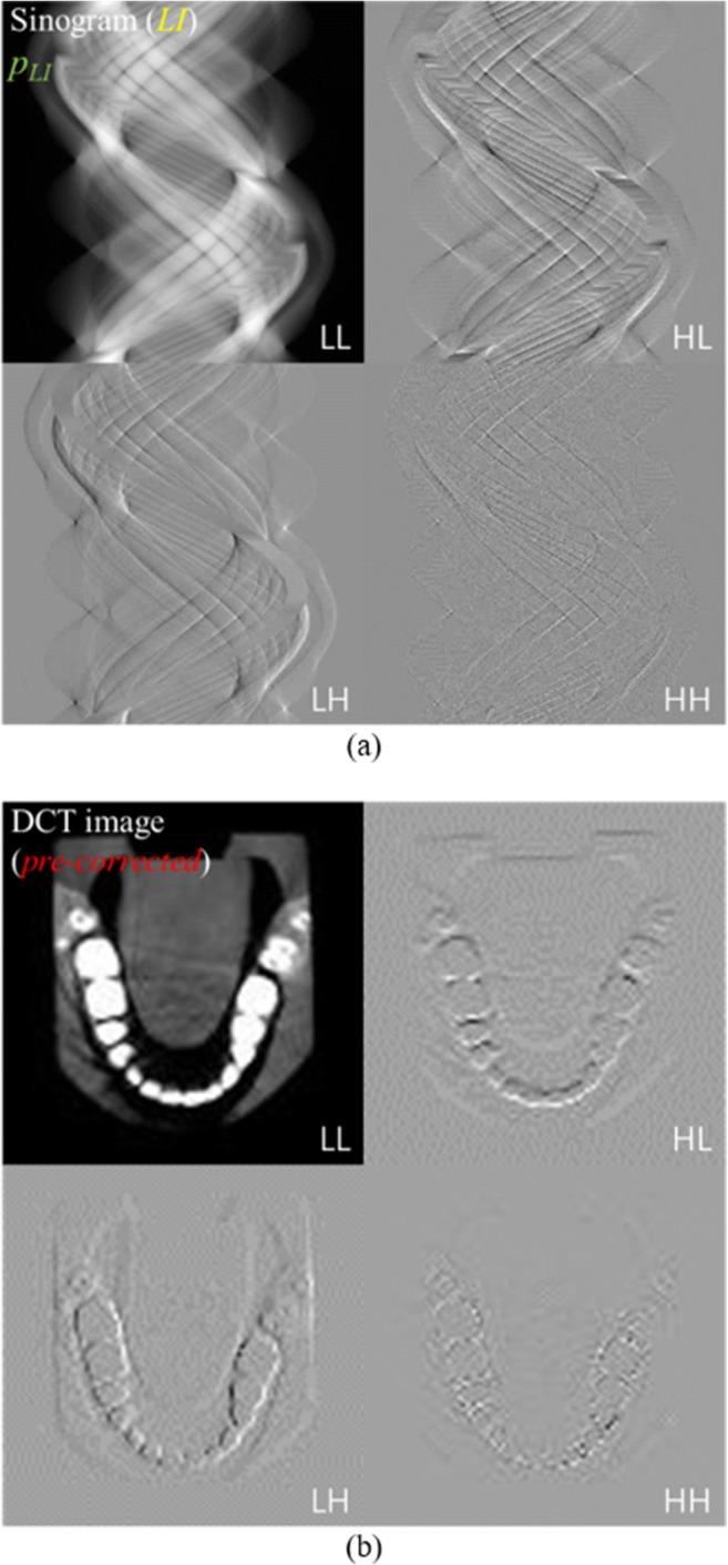
One-scale 2D DWT decomposition of the LI-interpolated sinogram (a) and FBP-reconstructed image (b) from the pre-corrected sinogram. A one-scale 2D DWT decomposed the input data before the feedforward to the network, and the inverse 2D DWT recomposed the predicted data after the network computation
Simulation and Experimental Preparation
To demonstrate the feasibility of the proposed MAR method, we performed a systematic simulation and an experiment with metal-inserted teeth phantoms. The table-top setup that we established in the study consisted of an X-ray tube, which was run at 60 kVp and 5 mAs, and a CMOS flat-panel detector with a pixel size of 198 μm (Fig. 4). Figure 5 shows the teeth phantom (lower mouth part of Kelvin™ phantom, CIRS Ltd.) (with no, one, two, and three metal inserts) used in the experiment and an example of the reconstructed slice images for each case of the metal inserts. The projection image for the no metal insert is also shown on the top middle. A three-dimensional numerical teeth phantom with a voxel dimension of 300 × 300 × 300 was used in the simulation. Five hundred forty projections were used to reconstruct DCT images using a voxel size of 0.4 mm through the standard filtered-backprojection (FBP) algorithm. The source-to-detector distance was 695 mm and the source-to-object distance was 409 mm. Details of the parameters used in the simulation and the experiment are listed in Table 1.
Fig. 4.
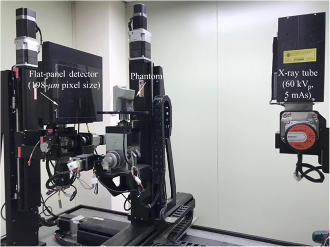
Table-top setup that we established in the study consisted of an X-ray tube, which was run at 60 kVp and 5 mAs, and a CMOS flat-panel detector with a pixel size of 198 μm
Fig. 5.

Teeth phantom (lower mouth part of Kelvin™ phantom, CIRS Ltd.) (with no, one, two, and three metal inserts) used in the experiment and an example of the reconstructed slice images for each case of the metal inserts. The projection image for the no metal insert is also shown on the top middle
Table 1.
Parameters used in the simulation and the experiment
| Parameter | Simulation | Experiment |
|---|---|---|
| Source-to-detector distance | 695 mm | 695 mm |
| Source-to-object distance | 409 mm | 409 mm |
| Number of projections | 540 | 540 |
| Voxel size | 0.4 mm | 0.4 mm |
| Pixel size | 0.198 mm | 0.198 mm |
| Phantom | Numerical teeth (300 × 300 × 300) | Physical teeth |
| Reconstruction algorithm | FBP | FBP |
We prepared the training and the test data using the numerical and the physical teeth phantoms for each simulation and experiment, respectively. Thirty-three DCT cases (i.e., 28 cases for the training and 5 cases for the test) with different metal positions of the data from the teeth phantoms were prepared for the simulation and the experiment. The sinograms and DCT images obtained from the teeth phantoms with no metal implants were used as the ground truth. The original sinograms were acquired from the teeth phantoms with metal implants and were used to generate LI-interpolated sinograms as input data in the sinogram completion network. The labeled data were prepared by subtracting the input data from the ground truth sinograms. In the sinogram completion network, 57,210 and 30,135 instances of the training data were present in the simulation and the experiment, respectively. We implemented data augmentation with a patch size of 256 × 256 and a stride of 128. Test data of 1527 and 402 sinograms were prepared in the simulation and the experiment, respectively. In the image completion network, the reconstructed DCT images from the corrected sinograms were used as the input data and the differences between the ground truth DCT images and the input data were used as the label data. The instances of the training data used in the simulation and the experiment totaled 9018 and 4671, respectively. The training data were also augmented with a patch size of 150 × 150 and a stride of 75. Test data of 840 and 218 DCT images were prepared in the simulation and the experiment, respectively. Both networks in the sinogram and the image domains were optimized using the adaptive momentum estimation (Adam) optimizer [21] and were trained on a normal computer with a GPU (Titan Xp, 12 GB) and a CPU (Intel Xeon, 3 GHz). The parameters used in the proposed FCN training are listed in Table 2.
Table 2.
Parameters used in the proposed FCN training
| Parameter | Sinogram domain | Image domain | ||
|---|---|---|---|---|
| Simulation | Experiment | Simulation | Experiment | |
| Learning rate | 10−3 | 10−3 | 10−3 | 10−3 |
| Number of epochs | 100 | 100 | 100 | 100 |
| Instances of the training data (augmented) | 57,210 | 30,135 | 9018 | 4671 |
| Amount of test data | 1527 | 840 | 402 | 218 |
| Training time (h) | 26 | 14 | 2 | 1 |
The image quality was evaluated quantitatively in terms of the root-mean-square error (RMSE) and the structural similarity (SSIM) [22]. The RMSE describes the correlation between the reconstructed (xrecon) and the original images (xorig) that is normalized to its maximum, and it is defined as follows:
| 5 |
where n is the number of pixels. A smaller RMSE ensures the maximum similarity with the original image values. The SSIM is popularly used for measuring the similarity between two images. It is defined as
| 6 |
where and σ are the mean and the standard deviation of the image values, respectively, and Cov represents the covariance; C1 and C2 are small positive constants that provide stability in the SSIM measurement. When the value of SSIM is closer to one, the two images under consideration are more similar.
Results and Discussion
Figure 6 shows the uncorrected DCT images of the numerical teeth phantom (third column) and their enlarged images inside box A (fourth column) with respect to the number of metal inserts. The corresponding phantom slice images are also shown on the left. The uncorrected images, as expected, suffered from severe metal artifacts (i.e., streaks and shadows) around the metal inserts as the number of metal inserts increased. The arrows in Fig. 6 indicate the position of the metal inserts.
Fig. 6.

Uncorrected DCT images of the numerical teeth phantom (third column) and their enlarged images inside box A (fourth column) with respect to the number of metal inserts. The corresponding phantom slice images are also shown on the left
Figure 7 shows the reconstructed DCT images of the numerical teeth phantom corrected using the NMAR (left), sFCN-MAR (middle), and proposed MAR (right) methods. Among the MAR methods, the proposed MAR considerably reduced the metal artifacts and corrected the images more accurately than the two other algorithms. The image improvement was more evident as the number of metal implants increased. The computational times consumed by the proposed MAR algorithm were approximately 32 s in the simulation and 23 s in the experiment. The detailed computational times for the proposed MAR algorithm in the simulation and the experiment are listed in Table 3.
Fig. 7.

Reconstructed DCT images of the numerical teeth phantom corrected using the NMAR (left), sFCN-MAR (middle), and proposed MAR (right) methods
Table 3.
Computational times for the proposed MAR algorithm
| Domain | Simulation (s) | Experiment (s) |
|---|---|---|
| Sinogram domain | 24 | 15 |
| Image domain | 8 | 8 |
Figure 8 shows the intensity profiles measured along in Fig. 7 for the DCT images reconstructed by using the NMAR, sFCN-MAR, and proposed MAR algorithms. The intensity profile of the phantom image is shown for comparison.
Fig. 8.

Intensity profiles measured along in Fig. 7 for the DCT images reconstructed by using the NMAR, sFCN-MAR, and proposed MAR algorithms. The intensity profile of the phantom image is shown for comparison
Figure 9 shows the (a) RMSE and (b) SSIM values measured from the reconstructed DCT images in Fig. 7 with respect to the number of metal inserts. It should be noted that the RMSE values were normalized to the RMSE value for the single metal insert with NMAR for easy comparison. The RMSE value of the proposed MAR method for three metal inserts was approximately 0.49, which was approximately 2.25 and 1.53 times smaller than those of the NMAR and the sFCN-MAR, respectively. The SSIM value of the proposed MAR was approximately 0.96, which was approximately 1.81 and 1.48 times larger than those of the NMAR and the sFCN-MAR, respectively. These results indicate that the proposed MAR method successfully suppressed the metal artifacts better than the NMAR and the sFCN-MAR methods.
Fig. 9.

RMSE (a) and SSIM (b) values measured from the reconstructed DCT images in Fig. 7 with respect to the number of metal inserts
We repeated the same MAR process using the experimental data. Figure 10 shows the reconstructed DCT images of the physical teeth phantom using the NMAR (left), sFCN-MAR (middle), and proposed MAR (right) methods. The experimental image results were similar to the simulation ones. The RMSE value of the proposed MAR method for the three metal inserts was approximately 0.69, which was approximately 2.49 and 1.53 times smaller than those of the NMAR and the sFCN-MAR, respectively. The SSIM value of the proposed MAR was approximately 0.93, which was approximately 1.11 and 1.06 times larger than those of the NMAR and the sFCN-MAR, respectively (Fig. 11). Here, the reconstructed image with no metal insert (shown on the top right in Fig. 5) was used as the reference image to measure the RMSE and the SSIM values in the experiment. Consequently, our results indicate that the proposed MAR method considerably reduced the metal artifacts by reducing the streak artifacts without any distortion in DCT images and demonstrated a better image performance than those of the NMAR and the sFCN-MAR methods.
Fig. 10.

Reconstructed DCT images of the physical teeth phantom using the NMAR (left), sFCN-MAR (middle), and proposed MAR (right) methods
Fig. 11.

RMSE (a) and SSIM (b) values measured from the reconstructed DCT images in Fig. 10 with respect to the number of metal inserts
Conclusion
This paper proposes a new deep learning–based method that uses a residual FCN to effectively reduce metal artifacts in DCT images. We performed a computational simulation and an experiment on a teeth phantom with several metal inserts to investigate the image quality and evaluate the effectiveness of the proposed method. According to our results, the proposed MAR method significantly reduced the metal artifacts, and its effectiveness was validated by comparing it with that of other methods such as the NMAR and the sFCN-MAR-based algorithms. The RMSE value for the proposed MAR with three metal implants in the simulation was approximately 2.25 and 1.53 times lower than those for the NMAR and the sFCN-MAR, respectively. Additionally, the SSIM value was approximately 0.96 for the proposed MAR algorithm. In the experiment, the RMSE value for the proposed MAR algorithm was 2.49 and 1.53 times smaller than those of the NMAR and the sFCN-MAR, respectively. Our simulation and experimental results indicate that the proposed MAR method reduced metal artifacts considerably in DCT images and showed better image performance than those of the NMAR and the sFCN-MAR methods in reducing streak artifacts without introducing any distortion. We expect that the proposed method can be useful for the reduction of metal artifacts in current real-world DCT systems.
Funding Information
This study was financially supported by the Basic Science Research Program through the National Research Foundation of Korea (NRF) funded by the Korea Ministry of Science and ICT (NRF-2017 R1A2B2002891).
Footnotes
Publisher’s Note
Springer Nature remains neutral with regard to jurisdictional claims in published maps and institutional affiliations.
References
- 1.Kataoka M, Hochman M, Rodrigues E, Lin P, Kudo S, Raptopolous V. A review of factors that affect artifact from metallic hardware on multi-row detector computed tomography. Curr. Probl. Diagn. Radiol. 2010;39:125–136. doi: 10.1067/j.cpradiol.2009.05.002. [DOI] [PubMed] [Google Scholar]
- 2.Veldkamp W, Joemai R, Molen A, Geleijns J. Development and validation of segmentation and interpolation techniques in sinograms for metal artifact suppression in CT. Med. Phys. 2010;37:620–628. doi: 10.1118/1.3276777. [DOI] [PubMed] [Google Scholar]
- 3.Olive C, Kaus M, Pekar V, Eck K, Spies L. Segmentation aided adaptive filtering for metal artifact reduction in radio-therapeutic CT images. Proc. SPIE. 2004;5370:1991–2002. doi: 10.1117/12.535346. [DOI] [Google Scholar]
- 4.Man B, Nuyts J, Dupont P, Marchal G, Suetens P. An iterative maximum-likelihood polychromatic algorithm for CT. IEEE Trans. Med. Imag. 2001;20:999–1008. doi: 10.1109/42.959297. [DOI] [PubMed] [Google Scholar]
- 5.Zhang Y, Yu H. Convolutional neural network based metal artifact reduction in X-ray computed tomography. IEEE Trans. Med. Imaging. 2018;37:1370–1381. doi: 10.1109/TMI.2018.2823083. [DOI] [PMC free article] [PubMed] [Google Scholar]
- 6.Hegazy M, Cho M, Lee S. A metal artifact reduction method for a dental CT based on adaptive local thresholding and prior image generation. BioMed. Eng. 2016;15:119–132. doi: 10.1186/s12938-016-0240-8. [DOI] [PMC free article] [PubMed] [Google Scholar]
- 7.Meyer E, Raupach R, Lell M, Schmidt B, Kachelrieß M. Normalized metal artifact reduction (NMAR) in computed tomography. Med. Phys. 2010;37:5482–5493. doi: 10.1118/1.3484090. [DOI] [PubMed] [Google Scholar]
- 8.Ghani M, Karl W: Fast enhanced CT metal artifact reduction using data domain deep learning. IEEE Trans. Comput. Imaging, 10.1109/TCI.2019.2937221, August 27, 2019
- 9.Park H, Lee S, Kim H, Seo J, Chung Y. CT sinogram-consistency learning for metal-induced beam hardening correction. Med. Phys. 2018;45:5376–5384. doi: 10.1002/mp.13199. [DOI] [PubMed] [Google Scholar]
- 10.Ghani M, Karl W. Deep learning based sinogram correction for metal artifact reduction. Electronic Imag. 2018;472:1–8. [Google Scholar]
- 11.Claus B, Jin Y, Gjesteby L, Wang G, Man B: Metal-artifact reduction using deep-learning based sinogram completion: initial results. Proc. 14th Int. Meeting Fully Three-Dimensional Image Reconstruction Radiol. Nucl. Med. 631–634, 2017
- 12.Gjesteby L, Yang Q, Xi Y, Zhou Y, Zhang J, Wang G: Deep learning methods to guide CT image reconstruction and reduce metal artifacts. Proc. SPIE 10132:101322W1–101322W7, 2017
- 13.Gjesteby L, Yang Q, Xi Y, Shan H, Claus B, Jin Y, Man B, Wang G: Deep learning methods for CT image-domain metal artifact reduction. Proc. SPIE 10391:103910W1–103910W6, 2017
- 14.Xu S, Dang H: Deep residual learning enabled metal artifact reduction. Proc. SPIE 10573:105733O1–105733O6, 2018
- 15.Zhu L, Han Y, Li L, Xu Y, Xi X, Yan B, Xiao K: Metal artifact reduction based on fully convolutional networks in CT image domain. Proc. SPIE 11068:110681U1–110681U7, 2018
- 16.Huang X, Wang J, Tang F, Zhong T, Zhang Y: Metal artifact reduction on cervical CT images by deep residual learning. Biomed Eng. 10.1186/s12938-018-0609-y, November 27, 2018 [DOI] [PMC free article] [PubMed]
- 17.Lee D, Choi S, Kim H. High quality imaging from sparsely sampled computed tomography data with deep learning and wavelet transform in various domains. Med. Phys. 2019;46:104–115. doi: 10.1002/mp.13258. [DOI] [PubMed] [Google Scholar]
- 18.He K, Zhang X, Ren S, Sun J: Deep residual learning for image recognition. IEEE CVPR 770–778, 2016
- 19.Kang E, Min J, Ye J. A deep convolutional neural network using directional wavelets for low-dose X-ray CT reconstruction. Med. Phys. 2017;44:e360–e375. doi: 10.1002/mp.12344. [DOI] [PubMed] [Google Scholar]
- 20.Heil C, Walnut D. Continuous and discrete wavelet transforms. SIAM Rev. 1989;31:628–666. doi: 10.1137/1031129. [DOI] [Google Scholar]
- 21.Kingma D, Ba J: Adam: a method for stochastic optimization. International Conference on Learning Representations. Available at http://arxiv.org/abs/1412.6980, 2014
- 22.Wang Z, Bovik A, Sheikh H, Simoncelli E. Image quality assessment: from error visibility to structural similarity. IEEE Trans. Image Proc. 2004;13:600–612. doi: 10.1109/TIP.2003.819861. [DOI] [PubMed] [Google Scholar]