Estimation of protein from the images of health drink powders

Abstract

Using new technologies to know the nutrition contents of food is the new emerging area of research. Predicting protein content from the image of food is one such area that will be most useful to the human beings because monitoring the nutrition intake has many health benefits. Patients with rare diseases like maple syrup urine disease need to be in good diet practices in order to survive. Protein intake has to be monitored for those individuals. In this paper, protein measurement of health drink powder is performed using image processing techniques. In this work food images are captured and a new database with 990 images of 9 health drink powders is created. Protein content is predicted using deep learning convolutional neural network and also using image features with linear regression. Image features like first order statistics, histogram-oriented gradient, gray level co-occurrence matrix, local binary pattern and gradient magnitude and gradient direction features obtained by applying Prewitt, Sobel and Kirsch are used to estimate the protein content. Training and testing are done using linear regression model which uses support vector machine to obtain the optimal hyper plane. A tenfold cross validation is used to improve the statistical significance of the results. Experimental results show that the protein contents are predicted with an average error of ± 2.71. Deep learning improves the prediction with an average error of ± 1.96.

Introduction

Nutrition is the process of providing food necessary for health and growth. It is the branch of science that deals with nutrients in food, how human body uses nutrients and how diet is related to health and diseases. It also deals with the interaction of nutrients and other substances in food with respect to maintenance, growth, reproduction, health and diseases. Food provides the necessary nutrients for survival and helps the body function and stay healthy. Nutrients are classified into two types: (1) Macronutrients and (2) Micronutrients. Macronutrients are carbohydrates, fiber, proteins, fats and water. Minerals and vitamins are micronutrients. Macronutrients offer calories to fuel the body. They play specific role in maintaining health. Proteins are structural materials which are the building blocks for the development, growth, and maintenance of body tissues. Protein provides structure to muscles and bones. There is no protein storage provision in human beings. Hence, amino acids must present in the everyday diet. Eating a balanced diet is vital for good health and wellbeing of humans. A wide variety of different foods is necessary to provide the right amount of nutrients for good health. An unhealthy diet increases the risk of many diet-related diseases. The consumption of unbalanced diet and improper nutrition may also lead to illness, disability and even death. Hence, nutrition plays an important role in the healthy life of humans.

Maple syrup urine disease is a rare genetic disease. Patients with maple syrup urine disease need to be treated with balanced diet. If untreated, may damage the brain and sometimes it may cause death. The medical treatment is normally a maintenance therapy which is assisting the patients’ dietary. In order to be in good diet practice the daily intake of protein need to be known. Hence protein measurement is essential.

One simple method to measure the nutrition intake is to recall the quantity and the type of food intake. Nutrition is predicted manually from the quantity and type of the food taken. The problem in this method is underestimation or overestimation of the food quantity (Livingston et al. 2004). According to Livingston et al. (2004) limited progress has been made to consider the error in reporting and estimating accurate nutrient intake. Problem of the error in reporting the intake of food can be reduced by maintaining the record of food intake. One of the earlier methods for recording the food intake is to use a diary and pencil. Problem in diary and pencil method is that it cannot be carried all the time. This causes delay in recording. This delay leads to the same reporting error. Therefore, Burke et al. (2005) suggested personal digital assistant and analyzed its advantages and disadvantages. The major advantage of this method is the digital nature of the report. The disadvantages are (1) training the user to use the personal digital assistant and (2) there may be reporting error as in the case of diary and pencil method, if the digital device is not possessed by the person all the time. In diary and pencil method as well as in personal digital assistant method, there is no guarantee that the quantity of the food is estimated accurately.

To overcome the problem of error in reporting and for the accurate estimation of food quantity, researchers showed interest in using image processing techniques. They worked towards predicting the nutrient content of food from its images.

In Sun et al. (2008), the amount of nutrients and calories of food have been predicted from its images. As a first step to prediction, the photograph of the food is captured along with a checkerboard calibration card. The checkerboard image is used to calculate the volume of the food. The type of food is identified by manual intervention. The volume of food and the type of food identified are used to predict the nutrients and calories using a lookup table. The need of the checkerboard to calculate the volume of the food and the manual intervention to identify the type of food are to be addressed to implement this method in real-time and make it user friendly. Also, the use of lookup table ignores the variation of nutrients and calories of food of the same type and volume.

Gao et al. (2009), captured the food image using a mobile phone camera. The captured food image is compared with image database to identify the type of food. The nutrients and calorie information are provided from a lookup table. This type of system is able to provide only the information about the type of food and the general nutrient content of the food.

Marriapan et al. (2009) addressed the problem of manual intervention for identifying the type of the food item by introducing a classification algorithm. Features like intensity, color and texture are extracted from the segmented food image and these features are used to predict the type of food using Support Vector Machine (SVM) classifier. But the prediction accuracy is 57.55%. As the prediction accuracy is low, it is necessary to verify and validate the prediction of SVM by manual intervention. Volume of food is calculated using a checkerboard method and nutrients are predicted using a lookup table similar to that of Sun et al. (2008). The use of lookup table to predict the nutrients and low classification accuracy in predicting the type of food are the areas to be addressed to make the system versatile. Use of more image features or combination of different image features may result in accurate prediction of food type.

Aizawa et al. (2013) estimated food-balance from food images and compared with Japanese food-balance guide which is similar to My Pyramid food-balance specification of the US Department of Agriculture (USDA). To estimate the food-balance, the food intakes of a person are recorded in the form of images. The images are classified as food image or non-food image and the food images are further classified into grains, vegetables, meat or fish or beans, fruit and dairy products using Naive classifier using combination of color, circle and bag of features. These categories are analyzed and compared with food-balance guide to give information about the nutritional intake.

For achieving the objective of measuring the calorie from food images, Pouladzadeh et al. (2014) identified the type of food with the help of SVM classifier using size, shape, color and texture features. From the food image, the volume of the food is measured and using the relation between volume and mass, the mass of the food is calculated. The type of food and its mass are used to predict the calorie from a lookup table. In this research, in order to measure the volume of the food from its image, the image of thumb is used instead of the checkerboard used in Sun et al. (2008) and Marriapan et al. (2009). In order to use the thumb to measure the food volume, it is necessary to capture the top and side view of the food by placing the thumb beside the food and we should know the volume of the thumb. When the volume of the food and lookup table are used to estimate the nutritional content, the estimation process becomes complicated for the image of mixed food items. In such cases, it is necessary to recognize the ingredients. Recognizing the ingredients from food image is another research area which is progressing (He et al. 2016). Anthimopoulos et al. (2015) estimated carbohydrates from food images by measuring the volume by capturing the image of food along with a reference card. A 3D shape of food image is reconstructed and the volume is estimated from the 3D image with the help of the reference card. The type of food is identified using radial basis support vector machine as classifier and histogram of colors and local binary pattern as features. Carbohydrate content is predicted by using USDA nutritional database as the lookup table. The estimation of carbohydrates from food images is further enhanced by measuring the volume using two view 3D reconstruction method Dehais et al. (2017).

Protein content of a single wheat kernel is estimated using hyper spectral imaging which is a combination of near-infrared spectroscopy and digital imaging (Caporaso et al. 2017). The spectra obtained from hyper spectral imaging are used to build partial least square regression model which is used to predict the protein content. The major advantages of the research work (Caporaso et al. 2017) are that the authors have predicted the protein content without calculating volume and without using a lookup table. Even though this research (Caporaso et al. 2017) is similar to the one proposed in this paper, it differs in the following aspects; (1) Caporaso et al. (2017) uses hyper spectral imaging but we use the simple photographic images, and (2) Caporaso et al. (2017) uses single grain of wheat but we use the food item as the whole.

Estimation of nutritional content of food from its images can play important role in a person’s day-to-day life, because capturing food images is very simple as everyone carries mobile phone with inbuilt camera. In the process of estimation of nutritional content from food images, the measurement of food volume makes the system less user-friendly, and the use of lookup table to predict the nutritional content does not consider the variation of the nutritional content of food of the same type and volume. People who are affected by disorders like Maple Syrup Urine Disease should know the amount of protein intake. These factors motivate us to predict nutritional content directly from the food images and for that purpose to create our own database.

The remainder of the paper is arranged as follows: "Image database for protein estimation" section explains the creation and description of the image database; "Image features extraction" section presents the features extracted from the images; "Protein estimation using image features" section explains the prediction of protein content experiments using image features; "Protein estimation using deep learning" section describes the prediction of protein content using deep learning; "Results and discussion" section presents the prediction results and "Conclusion and future work" section concludes the paper.

Image database for protein estimation

A new image database called Image Database for Protein Estimation (IDPE) is created for protein prediction from food images. The database has 990 images captured using an Android phone. The database is formed from 9 food items. Among the 9 food items, six food items are milk powders which are used for children under 3 years and the remaining 3 food items are health drink powders. The brand name of the chosen food items are Lactogen, Nan, Similac, Farex, Dexolac, Horlicks, Boost, Bournvita and Complan, available in the Indian market. The images are captured at different heights and at different angles. The food items are weighed using a notebook-weighing machine. Food items are weighed such that they weigh 1, 2, 3, 5, 8, 10, 12, 15, 20 and 25 g. All the weighted food items are bust shorted from 11 different positions using 13 MP camera of Redmi note 4 Android phone. The first three shots are the top view of the food item at three different heights. Fourth and fifth shots are taken from one side at two different angles. Similarly, another 2 photos are captured at different angles from each of the remaining 3 sides. Hence, for each weighted food item, 11 images are captured.

The captured images are named in such a way that the file names represent the name of the food item they belong to, the weight, the image-capturing position, image capturing height/angle and the amount of protein present per 100 g. In the file name, the first three letters represent the brand name of the food. Fourth and fifth positions represent the weight of the food item in grams. Sixth and seventh positions represents whether the image is captured from the top or the side. TP is used to represent top, S1 is used to represent first side, S2 is used to represent the second side, S3 is used to represent the third side and S4 is used to represent the fourth side. Eighth position represents the height for top view and the angle for the side view. Low height is represented by L, medium height is represented by M and high height is represented by H. For the food images photographed from the sides, 1 is used to represent one vertical angle and 2 is used to represent the second vertical angle. The ninth to thirteenth positions represent the amount of protein content per 100 g. Table 1 shows the brand names of the food items, the abbreviation used in file names and the amount of protein present in the food items.

Table 1.

Food items and the protein content

Brand name of the food item	Abbreviation	Protein content per 100 g
Lactogen	LAC	14.20
Nan	NAN	14.30
Similac	SIM	14.50
Farex	FAR	16.00
Dexolac	DEX	16.00
Horlicks	HOR	11.00
Boost	BOO	07.50
Bournvita	BOU	07.00
Complan	COM	18.00

For example, in the image file name BOO01TPL07.50, the brand name of the food item is Boost (BOO), the weight of the food item is 1 g (01), the image is captured from the top (TP), the image is captured by placing the camera at lower height from the food item (L) and the protein content per 100 g is 7.5 (07.50).

Images of the database are in JPG format having 3120 pixels width and 4160 pixels height. Horizontal as well as vertical resolution of the images is 72 dpi. Bit depth of the pixel is 24.

Researchers who wish to use IDPE for noncommercial research work can obtain the database by sending a request to the authors.

Image features extraction

Image features are the pieces of information that represent the characteristics of the image. Shape, color, texture, size and contrast are some of the examples of features. Color is one of the most important features and can be obtained from the color histogram. Rotation, resizing and zooming do not affect the color features of an image; hence color features are an efficient one. In a large image, for analyzing the repetitive structure, texture features can be extracted. Shape features can be obtained by contour method or region- based methods. In this section, the various features like First Order Statistics (FOS), Histogram of Oriented Gradient (HOG), Local Binary Pattern (LBP), Gray Level Co-occurrence Matrix (GLCM) and statistics of gradient magnitude and gradient direction extracted from the food images for the purpose of protein content prediction are explained.

First order statistics

Properties of individual pixel of an image are estimated by first order statistics. The texture of an image region is determined by the way the gray levels are distributed over the pixels in the region. First order statistics based features are described to quantify properties of an image region by using the relations underlying the gray level distribution of a given image. Some of the first order features derived from the images are mean, standard deviation, skewness, kurtosis and entropy. Calculations of these features from average histogram of gray levels are explained below.

Let the random variable I represent the gray levels of the pixels of an image region. The first order histogram H(I) is obtained as the number of pixels with gray level I to the total number of pixels in the region. Equation (1) shows the mathematics involved in the calculation of the mean feature E[I].

$$Mean=E\left[I\right]=\sum _{I=0}^{N}I·H\left(I\right)$$ 1

where N represents the number of possible gray levels.

Most often used central moments are variance, standard deviation, skewness and kurtosis. The variance is the measure of the width of the histogram i.e. measure of deviation of gray levels from the mean. The square root of the variance is the standard deviation. Gray level variance of the image region is calculated using Eq. (2).

$$Variance=E\left[I-E{\left[I\right]}^2\right]$$ 2

Standard deviation of the gray levels of the image region is calculated by taking square root of the Eq. (2).

Skewness is the measure of the degree of histogram asymmetry around the mean. Skewness of an image is obtained using Eq. (3).

$$Skewness=E\left[I-E{\left[I\right]}^3\right]$$ 3

Kurtosis is a measure of the histogram sharpness and used to measure the presence of outliers. Kurtosis is obtained using Eq. (4).

$$Kurtosis=E\left[I-E{\left[I\right]}^4\right]$$ 4

Image entropy is a feature that provides information about the intensity levels of image pixels. Entropy from histogram is calculated using Eq. (5).

$$Entropy=-\sum P\left(I\right){log}_{2}P\left(I\right)$$ 5

where P(I) is the probability of intensity value I.

Histogram of oriented gradient

Shapes within an image can be characterized by distribution of intensity gradients. This is based on evaluating normalized local histograms of image gradient orientations. Histogram of oriented gradients of food images are extracted as given below. Food image is divided into 8 × 8 cells. Horizontal and vertical unsigned gradients for each pixel of each cell are calculated. Magnitude and angle of unsigned gradients of each cell are represented by a histogram with 9 bins. The 9 bins represent the angles 0, 20, 40, 60, 80, 100, 120, 140 and 160 degrees. If the angle of a gradient is any one of the above angles, the whole magnitude of the gradient is added to the corresponding bin. If the angle of a gradient is other than the above angles, the magnitude will be divided proportionately into two and added to two bins. The bins and the division proportion are decided by the angle. The histogram of gradients of each cell is normalized over a block size of 16 × 16 i.e. each block consists of 4 cells. Therefore, the normalized histogram is an array of 36 elements. The size of the input food image to the HOG extraction process is 256 × 256. There are 961 normalization blocks; therefore, HOG of a food image has 34,596 elements.

Local binary pattern

LBP gives the texture details of an image. The formation of LBP feature vector is simple. First, the image is divided into number of cells. In every cell each pixel is compared with its 8 neighbors either in clockwise or anti clockwise direction. A LBP is obtained by placing a 0 when the center pixel is greater than the neighboring pixel, otherwise a 1 is appended. So an 8-bit binary number is formed which is converted to decimal. Then the histogram is computed over the cell. 59 LBP’s are obtained from the database images.

Gray level co-occurrence matrix

GLCM is extracted by considering the spatial relationship between pixels and it provides the texture information of an image. Elements of GLCM are the number of occurrence of each pair of pixels with specific values. GLCM is a matrix with a number of rows and columns equal to the number of individual gray levels in the image. Using this matrix co-occurrence features are defined which quantifies coarseness, smoothness and texture. The gray co-matrix formed is an 8 × 8 matrix from which the features can be derived. Some of the common statistics derived from GLCM are energy, homogeneity, contrast and correlation. In the current work, from each image of the IDPE, 23 derived features are extracted from each image. The statistical measures computed are autocorrelation, contrast, correlation 1, correlation 2, cluster prominence, cluster shade, dissimilarity, energy, entropy, homogeneity 1, homogeneity 2, maximum probability, sum of squares, sum average, sum variance, sum entropy, difference variance, difference entropy, information measures of correlation 1, information measures of correlation 2, inverse difference in homogeneity, inverse difference normalized and inverse difference in moment normalized.

Gradient magnitude and gradient direction

One of the feature considered for the prediction of protein is by the use of gradient values. For this purpose, the Prewitt mask is used which detects the 2D spatial gradient values. This produces the first order derivative of intensity values. Here the direction of largest possible change in the intensity can be found. Abrupt or smooth feature changes at a point can be analyzed using the Prewitt mask. Mathematically, the Prewitt operator uses 2 kernels each with 3 × 3 in size. Convolution of kernel and original image produces the gradient values one in horizontal and another in vertical direction.

Let the gradient be denoted as ∇I for an image I(x, y) at a location defined at (x, y).Also G_x and G_y be the horizontal and vertical derivatives of the image I. G_x and G_y are obtained as follows.

$$\mathrm{\nabla }\text{I}=\left[\begin{array}{c}{G}_x\\ G_y\end{array}\right]=\left[\begin{array}{c}\frac{\partial I}{\partial x}\\ \frac{\partial I}{\partial y}\end{array}\right]$$ 6

The gradient magnitude and gradient direction $\alpha \left(x,y\right)$ can also be obtained as follows

$$mag\left(\mathrm{\nabla }I\right)={\left[G_x^2{G}_y^2\right]}^{\raisebox{1ex}{$1$}\!\left/ \!\raisebox{-1ex}{$2$}\right.}$$ 7

$$\alpha \left(x,y\right)={tan}^{-1}\left(G_y/G_x\right)$$ 8

The two kernels used in Prewitt operator are shown in Fig. 1.

Fig. 1.

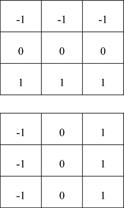
Kernels of Prewitt operator

The statistical measures computed from the gradient magnitude and gradient direction obtained using Eqs. 6, 7 and 8 are the mean, standard deviation and the correlation.

Features like FOS, HOG, LBP, GLCM, statistical features using Gradient Magnitude and Gradient Direction are extracted from the full color image, red component image, green component image, blue component image and gray image of the food images of IDPE.

Protein estimation using image features

The experiment of prediction of protein content from food images consists of three major steps as shown in Fig. 2. The first one is the capture of the image of the food item. Database of images with known protein content is formed. The second step is the extraction of features from the images. Image features like First Order Statistics, Histogram Oriented Gradient, Local Binary Pattern, Gray Level Co-occurrence Matrix, statistics of Gradient Magnitude and Gradient Direction are extracted. In the third step, linear regression model with support vector machine is used to gain the protein content knowledge and predict the protein content from the image features.

Fig. 2.

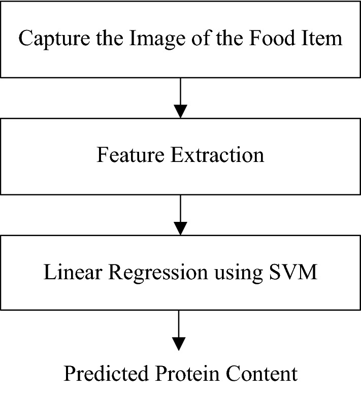
Different phases of protein prediction from food mages

In the experimentation of predicting protein content from food images using linear regression, the protein content is the independent variable and the image feature is the dependent variable. During the training phase, the model studies the relationship between image features and protein content and gain knowledge. During the testing phase, the trained model predicts the protein content from the features of food image. We use linear regression with support vector machine. Support vector machine is used to find the optimum hyper planes with maximum margin.

Statistical significance of the prediction results is improved by using tenfold cross validation scheme. In tenfold cross validation, the features are divided into 10 mutually exclusive uniform sets. The regression model is trained with 9 sets and tested with the remaining one set. This training and testing process is repeated 10 times so that each of the 10 sets acts as the test set one time. Results of each turn of tenfold cross validation are averaged to produce a single estimation. The advantages of tenfold cross validation are that (1) all the data are used for both training and testing (2) it is like doing the experiments with 10 different data sets and (3) it is like doing the experiment with large data set.

Protein prediction experiments are done separately with full color image, red component image, green component image, blue component image and gray image. For each image component, five image features such as FOS, HOG, LBP, GLCM and Prewitt Gradient are extracted. The features are used in two ways. In the first experiment, each feature of each image component is tested for protein prediction performance. A total of 22 experiments are done as shown in the Table 2. This type of experiments helps to identify which image feature of which image component is best in predicting protein content.

Table 2.

Average prediction error obtained by single feature of single image component

Image component	Average prediction error
	Image feature
	FOS	HOG	LBP	GLCM	Prewitt
Full color component	± 3.02	± 3.60	–	–	–
Red color component	± 2.86	± 3.39	± 3.13	± 2.80	± 2.90
Green color component	± 2.81	± 3.48	± 3.08	± 2.80	± 2.90
Blue color component	± 2.89	± 3.14	± 3.05	± 2.71	± 2.98
Gray component	± 2.82	± 3.98	± 3.11	± 2.80	± 3.03

In the second experiment, the combinations of features are tested for their protein prediction performance. In this case of experiments, the combinations of features like FOS + HOG, FOS + LBP, FOS + GLCM, FOS + Prewitt, HOG + LBP, HOG + GLCM, HOG + Prewitt, LBP + GLCM, LBP + Prewitt and GLCM + Prewitt combinations of each image components are tested. A total of 41 experiments are done as shown in Table 3. These types of experiments help to check whether the combination of features improves the prediction accuracy and to find the feature combination which improves the prediction performance.

Table 3.

Average prediction error obtained by combination features of single image component

Image feature combination	Average prediction error
	Image component
	Full component	Red component	Green component	Blue component	Gray component
FOS + HOG	± 3.52	± 3.14	± 3.05	± 3.46	± 3.28
FOS + LBP	–	± 3.35	± 3.23	± 2.87	± 3.15
FOS + GLCM	–	± 2.81	± 2.81	± 2.81	± 2.80
FOS + Prewitt	–	± 2.89	± 2.91	± 2.94	± 2.79
HOG + LBP	–	± 3.31	± 3.38	± 3.60	± 3.55
HOG + GLCM	–	± 4.56	± 4.34	± 3.46	± 4.63
HOG + Prewitt	–	± 3.72	± 3.56	± 4.72	± 4.38
LBP + GLCM	–	± 2.80	± 2.80	± 3.06	± 2.82
LBP + Prewitt	–	± 2.94	± 2.78	± 2.84	± 2.90
GLCM + Prewitt	–	± 3.23	± 3.74	± 3.60	± 3.83

In the third experiment, for each color component, the image features which predicted the protein content with error less than ± 3 are combined and tested for their prediction accuracy.

Protein estimation using deep learning

Deep learning neural network is a promising tool in the area of classification and regression. In deep learning, images can be fed directly as the input. The algorithm which we used in the estimation of protein from the health drink powders is deep convolutional neural network. The protein prediction experiments are conducted in train-test method. 70% images of the IDPE database are used for training the deep convolutional neural network and the remaining 30% images are used for testing and analyzing the performance.

Deep convolutional neural network is formed with (1) image input layer, (2) convolutional layer, (3) normalization layer, (4) linear rectification layer, (5) pooling layer, (6) fully connected layer and (7) regression layer. Image input layer is designed to handle the size of the input image and the number of channels per image. Convolution layer is designed with image filter of size 3 × 3 and configured for 25 numbers of convolutional filtering operations. The convolutional layer forms a stack of 25 filtered images. Normalization layer is used to normalize the convolved images. Linear rectification layer acts as the activation function and thresholds the filtered images in such a way that they have only zeros and positive values. The convolved and rectified images are down sampled using the pooling layer. Here, pooling layer is designed with a mask of size 2 × 2 and slide of 16 pixels to select the maximum from the masked region. Fully connected layer with one output followed by a regression layer is used.

Training of the deep convolutional neural network is done based on the steepest descent algorithm with 30 as well as 40 epochs and at a learning rate of 0.001. Protein prediction experiments with deep convolutional neural network are done separately with full color component, red channel, green channel, blue channel and gray images.

Results and discussion

Average prediction errors obtained by training and testing linear regression with each image feature of each image component are shown in Table 2. The results show that GLCM features of blue component of image predict protein with minimum average error of ± 2.71. FOS, GLCM and Prewitt features of green, red, blue and gray components perform better than HOG and LBP features. It is inferred from the results that texture feature like GLCM is good in predicting protein content. On the other hand, the HOG features are the worst predictor.

Average prediction errors obtained by training and testing linear regression with each combination of image features of each of the five image components are shown in Table 3. The results show that LBP and Prewitt features combination of green color component of image predicts protein with average error of ± 2.78. FOS and GLCM features combination of all the color components performs better than the other combinations. In the features combination analysis also it is inferred from the results that texture features like LBP and GLCM are good in predicting protein content and HOG predicts with maximum average error.

The average prediction errors obtained by training and testing linear regression with each combination of features of single image component having average prediction error less than ± 3.00 is shown in Table 4. The experimental results show that the combination of features reduces the prediction accuracy except in the case of gray component.

Table 4.

Average prediction error obtained by combination of features of single image component having average prediction error <  ± 3.00

Image component	Image feature combination	Average prediction error
Red color component	FOS + GLCM + Prewitt	± 3.22
Green color component	FOS + GLCM + Prewitt	± 3.89
Blue color component	FOS + GLCM + Prewitt	± 3.58
Gray component	FOS + GLCM	± 2.80

Average prediction errors obtained using different components of the input images by the deep convolutional neural network are shown in Table 5. Protein prediction with deep learning improves the prediction accuracy. The minimum average prediction error obtained with deep learning is ± 1.96 using full color component images. Blue channel of the images with deep learning also predicts the protein well with an average error of ± 1.97.

Table 5.

Average protein prediction errors obtained by using deep convolutional neural network

Image component	Average prediction error
	With 30 epoch	With 40 epoch
Full color component	± 2.13	± 1.96
Red color component	± 2.13	± 2.12
Green color component	± 2.03	± 2.01
Blue color component	± 1.97	± 1.98
Gray component	± 2.04	± 2.01

Research works done so far in food image processing use database images with fruits, mixed fruits and other restaurant menus. Our work is a unique one in which the experiments have been done using a new image database of health drink powders. We have obtained good prediction accuracy. We would like to further investigate to improve the protein content prediction accuracy using photographic images. The prediction accuracy will improve if microscopic images are used, but we need a technology to include microscope in mobile phones so that common people can also use it and predict accurately the protein content of their food intake.

Conclusion and future work

In this research work, a database of food images having 990 images is created. The database consists of the images of 11 postures of 9 different food items in different measurements. Prediction of protein content of food items is done by using first order statistics, histogram of oriented gradient, linear binary pattern, gray level co-occurrence matrix, gradient magnitude and gradient direction features using linear regression model with support vector machine. A minimum average protein prediction error of ± 2.71 is observed when GLCM feature extracted from the blue color component is used to model the linear regression system and a minimum average protein prediction error of ± 1.96 is observed in full color component when deep convolutional neural network is used to model the regression system. Deep neural network shows improved protein prediction.

We would like to investigate further with more layers in the deep convolutional neural network, by taking more features, especially a feature that carries the characteristic change information of light when it is reflected by protein to improve the protein prediction accuracy, and also by extending the current research database by using various other food images like fruits, vegetables, mixed food etc.

References

- Aizawa K, Maruyama Y, Li H, Morikawa C. Food balance estimation by using personal dietary tendencies in a multimedia food log. IEEE Trans Multimed. 2013;15(8):2176–2185. doi: 10.1109/TMM.2013.2271474. [DOI] [Google Scholar]
- Anthimopoulos M, Dehais J, Shevchik S, Ransford BH, Duke D, Diem P, Mougiakakou S. Computer vision-based carbohydrate estimation for type 1 diabetic patients using smartphones. J Diabetes Sci Technol. 2015;9(3):507–515. doi: 10.1177/1932296815580159. [DOI] [PMC free article] [PubMed] [Google Scholar]
- Burke LE, Warziski M, Starrett T, Choo J, Music E, Serika S, Stark S, Sevick MA. Self-monitoring dietary intake: current and future practices. J Renal Nutr. 2005;15(3):281–290. doi: 10.1016/j.jrn.2005.04.002. [DOI] [PubMed] [Google Scholar]
- Caporaso N, Whitworth MB, Fisk ID. Protein content prediction in single wheat kernels using hyperspectral imaging. Food Chem. 2017;240:32–42. doi: 10.1016/j.foodchem.2017.07.048. [DOI] [PMC free article] [PubMed] [Google Scholar]
- Dehais J, Anthimopoulos M, Shevchik S, Mougiakakou S. Two-view 3D reconstruction for food volume estimation. IEEE Trans Multimed. 2017;19(5):1090–1099. doi: 10.1109/TMM.2016.2642792. [DOI] [Google Scholar]
- Gao C, Kong F, Tan J (2009) Healthware: tackling obesity with health aware smart phone systems. In: IEEE international conference on robot, Guilin, China. 10.1109/ROBIO.2009.5420399
- He H, Kong F, Tan J. Multiview food recognition using multikernal SVM. IEEE J Biomed Health Inform. 2016;20(3):848–855. doi: 10.1109/JBHI.2015.2419251. [DOI] [PubMed] [Google Scholar]
- Livingstone MBE, Robson PJ, Wallace MW. Issues in dietary intake assessment of children and adolescents. Br J Nutr. 2004;92(2):213–222. doi: 10.1079/BJN20041169. [DOI] [PubMed] [Google Scholar]
- Mariappan A, Bosch M, Zhu F, Boushey CJ, Kerr DA, Ebert DS, Delp EJ (2009) Personal dietary assessment using mobile devices. In: Proceedings of SPIE electronic imaging, San Jose, California, United States. 10.1117/12.813556 [DOI] [PMC free article] [PubMed]
- Pouladzadeh P, Shirmohammadi S, Al-Maghrabi R. Measuring calorie and nutrition from food image. IEEE Trans Instrum Meas. 2014;63(8):1946–1956. doi: 10.1109/TIM.2014.2303533. [DOI] [Google Scholar]
- Ministry of Agriculture, Forestry and Fisheries of Japan, Food Balance Guide. https://www.maff.go.jp/j/balance_guide/. Referred on 05 Aug 2018
- Sun M, Liu Q, Schmidt K, Yang J, Yao N, Fernstrom JD, Fernstrom MH, DeLany JP, Sclabassi RJ (2008) Determination of food portion size by image processing. In: Proceedings of the 30th annual international conference of the engineering in medicine and biology society, Vancouver, British Columbia, Canada. 10.1109/IEMBS.2008.4649292 [DOI] [PubMed]
- United States Department of Agriculture, MyPlate and Food Pyramid Resources. https://fnic.nal.usda.gov/dietary-guidance/. Referred on 08 Aug 2018