Toward Asymptotically-Optimal Inspection Planning via Efficient Near-Optimal Graph Search

Abstract

Inspection planning, the task of planning motions that allow a robot to inspect a set of points of interest, has applications in domains such as industrial, field, and medical robotics. Inspection planning can be computationally challenging, as the search space over motion plans grows exponentially with the number of points of interest to inspect. We propose a novel method, Incremental Random Inspection-roadmap Search (IRIS), that computes inspection plans whose length and set of successfully inspected points asymptotically converge to those of an optimal inspection plan. IRIS incrementally densifies a motion planning roadmap using sampling-based algorithms, and performs efficient near-optimal graph search over the resulting roadmap as it is generated. We demonstrate IRIS’s efficacy on a simulated planar 5DOF manipulator inspection task and on a medical endoscopic inspection task for a continuum parallel surgical robot in cluttered anatomy segmented from patient CT data. We show that IRIS computes higher-quality inspection plans orders of magnitudes faster than a prior state-of-the-art method.

I. INTRODUCTION

We consider the problem of inspection planning, or coverage planning [1, 19]. Here, we consider the specific setting where we are given a robot equipped with a sensor and a set of points of interest (POI) in the environment to be inspected by the sensor. The problem calls for computing a minimal-length motion plan for the robot that maximizes the number of POI inspected. This problem has a multitude of diverse applications, including industrial surface inspections in production lines [43], surveying the ocean floor by autonomous underwater vehicles [3, 20, 26, 52], structural inspection of bridges using aerial robots [4, 5], and medical applications such as inspecting patient anatomy during surgical procedures [32], which motivates this work.

Naïvely-computed inspection plans may enable inspection of only a subset of the POI and may require motion plans orders of magnitude longer than an optimal plan, and hence may be undesirable or infeasible due to battery or time constraints. In medical applications, physicians may want to maximize the number of POI inspected for diagnostic purposes. Additionally, the procedure should be completed as fast as is safely possible to reduce costs and improve patient outcomes, especially if the patient is under anesthesia during the procedure. For example, a robot assisting in the diagnosis of the cause of a pleural effusion (a serious medical condition which causes the collapse of a patient’s lung) will need to visually inspect the surface of the collapsed lung and chest wall inside the body in as short a time as possible (see Fig. 1). We note that it may not be possible to inspect some POI due to obstacles in the anatomy and the kinematic constraints of the robot. Our goal is to compute high-quality inspection plans that maximize the number of POI inspected, and of the motion plans that inspect those POI we compute a shortest plan that is kinematically feasible and avoids obstacles.

Fig. 1:

Inspection planning in human anatomy. Top Left: The Continuum Reconfigurable Incisionless Surgical Parallel (CRISP) robot [2, 38] is composed of needle-diameter tubes assembled into a parallel structure inside the patient’s body (in which a tube uses a snare system to grip a tube with a camera affixed to its tip) and then robotically manipulated outside the body, allowing for smaller incisions and faster recovery times compared to traditional endoscopic tools (which have larger diameters). Top Right: The CRISP robot in simulation inspecting a collapsed lung, a scenario segmented from a CT scan of a real patient with this condition. The visualization shows the robot (orange), the lungs (pink), and the pleural surface visible (green) and not visible (blue) by the robot’s camera sensor in its current configuration. Bottom: Our method, IRIS, constructs a tree representing collision-free configurations (orange nodes) and motions (solid lines) of the robot. For each node, the robot (orange) can see points of interest (yellow) on the segmented anatomy (blue). IRIS then searches over an implicit graph structure (dashed lines) to compute asymptotically-optimal inspection plans.

Inspection planning is computationally challenging because the search space is embedded in a high-dimensional configuration space $\mathcal{X}$ (space of all parameters that determine the shape of the robot) [10, 33, 34]. Even finding the shortest plan between two points in $\mathcal{X}$ that avoid obstacles (without reasoning about inspection) is computationally hard.¹ If we want a minimum-length motion plan that maximizes the number of POI inspected, our problem is accentuated as we have to simultaneously reason about the system’s constraints, motion plan length, and POI inspected.

There are multiple approaches to computing inspection plans. Optimization-based methods locally search over the space of all inspection plans [4, 7]. Decoupled approaches first independently select suitable viewpoints and then determine a visiting sequence, i.e., a motion plan for the robot that realizes this sequence [11, 17]. Finally, recent progress in motion planning [28] has enabled methods to exhaustively search over the space of all motion plans [6, 27, 41] thus guaranteeing asymptotic optimality, a key requirement in many applications, including medical ones. Roughly speaking, asymptotic optimality for inspection planning means these methods produce inspection plans whose length and number of points inspected will asymptotically converge to those of an optimal inspection plan, given enough planning time.

Of all the aforementioned methods, only algorithms in the latter group provide any formal guarantees on the quality of the solution. This guarantee is achieved by attempting to exhaustively compute the set of Pareto-optimal inspection plans embedded in $\mathcal{X}$. In our setting, the set of Pareto-optimal inspection plans is the minimal set of inspection plans such that each plan is either shorter or has better coverage of the POI than any other inspection plan². Unfortunately, this comes at the price of very long computation times as the search space is exponential in the number of POI.

To this end, we introduce Incremental Random Inspection-roadmap Search (IRIS), a new asymptotically-optimal inspection-planning algorithm. IRIS incrementally constructs a sequence of increasingly dense roadmaps—graphs embedded in $\mathcal{X}$ wherein each vertex represents a collision-free configuration and each edge a collision-free transition between configurations—and computes an inspection plan on the roadmaps as they are constructed (see Fig. 2). Unfortunately, even the problem of computing an optimal inspection plan on a graph (and not in the continuous space) is computationally hard. To this end, our key insight is to compute a near-optimal inspection plan on each roadmap. Namely, we compute an inspection plan that is at most 1 + ε the length of an optimal plan while covering at least p-percent of the number of POI (for any ε ≥ 0 and p ∈ (0, 1]). This additional flexibility allows us to improve the quality of our inspection plan in an anytime manner, i.e., the algorithm can be stopped at any time and return the best inspection plan found up until that point. We achieve this by incrementally densifying the roadmap and then searching over the densified roadmap for a near-optimal inspection plan—a process that is repeated as time allows. By reducing the approximation factor between iterations, we ensure that our method is asymptotically optimal.

Fig. 2:

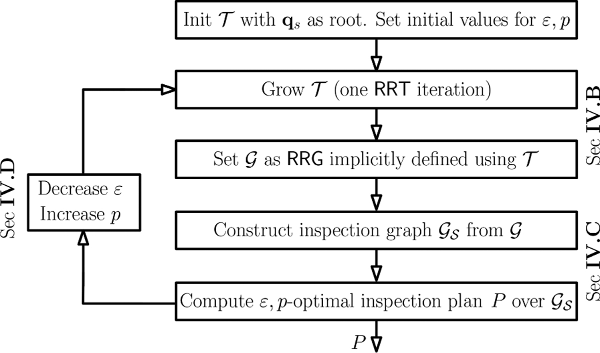
Overview of the IRIS algorithmic framework

The key contribution of our work is a computationally-efficient algorithm to compute provably near-optimal inspection plans on graphs. By pruning away large portions of the search space, this algorithmic building block enables us to dramatically outperform Rapidly-exploring Random Tree Of Trees (RRTOT) [6]—a state-of-the-art asymptotically-optimal inspection planner. Specifically, we demonstrate the efficacy of our approach in simulation for a continuum robot with complex dynamics—the needle-diameter Continuum Reconfigurable Incisionless Surgical Parallel (CRISP) robot [2, 38], working in a medically-inspired setting involving diagnosis of a pleural effusion (see Fig. 1).

II. RELATED WORK

A. Sampling-based motion planning

Motion planning aims to compute a collision-free motion for a robot to accomplish a task in an environment cluttered with obstacles [22, 34, 37]. A common approach to motion planning is by sampling-based algorithms that construct a roadmap. Examples include the Probabilistic Roadmaps (PRMs) [29] (for solving multiple queries) and the Rapidly-exploring Random Trees (RRTs) [35] for solving single queries. These methods, and many variations thereof, are probabilistically complete—namely the likelihood that they will find a solution, if one exists, approaches certainty as computation time increases.

Recent variations of these methods, such as PRM* and RRT* [28], improve upon this guarantee by exhibiting asymptotic optimality—namely that the quality of the solution obtained, given some cost function, approaches the global optimum as computation increases. Roughly speaking, this is achieved by increasing the (potential) edge set of roadmap vertices considered as its size increases [28, 50]. One such algorithm is the Rapidly-exploring Random Graphs (RRGs) [28] which will be used in our work. RRG combines the exploration strategy of RRT with an updated connection strategy that allows for cycles in the roadmap. It requires solving the two-point boundary value problem [34], which is only available for some robotic systems (including ours).

Guaranteeing asymptotic optimally can come with heavy computational cost. This inspired work on planners that trade asymptotic optimality guarantees with asymptotic near optimality (e.g., [36, 39, 47]). Asymptotic near optimality states that given an approximation factor ε ≥ 0, the solution obtained converges to within a factor of (1+ε) of the optimal solution with probability one, as the number of samples tends to infinity. Relaxing optimality to near optimality allows a method to improve the practical convergence rate while maintaining desired theoretic guarantees on the quality of the solution.

B. Inspection planning

Many inspection-planning algorithms, or coverage planners, decompose the region containing the POI into multiple subregions, and then solve each sub-region separately [19]. These methods have limitations, however, such as when occlusions play a significant role in the inspection [16], or when kinematic constraints must be considered [14].

Other approaches simultaneously consider all POI. One approach decouples the problem into the coverage sampling problem (CSP) and the multi-goal planning problem (MPP), and solves each independently [4, 11, 14, 16, 17]. In CSP, a minimal set of viewpoints that provide full inspection coverage is computed. In MPP, a shortest tour that connects all the viewpoints is computed. These corresponds to solving the art gallery problem and the traveling salesman problem, respectively. Several of these variants have been shown to be probabilistically complete [16], but none provide guarantees on the quality of the final solution.

The set of viewpoints and the inspection plan itself can also be generated simultaneously. Papadopoulos et al. propose the Random Inspection Tree Algorithm (RITA) [41]. RITA takes into account differential constraints of the robot and computes both target points for inspection and the trajectory to visit the targets simultaneously. Bircher et al. propose Rapidly-exploring Random Tree Of Trees (RRTOT) which constructs a metatree structure consisting of multiple RRT* trees [6]. Both methods, which were shown to be asymptotically optimal, iteratively generate a tree, in which the inspection plan is enforced to be a plan from the root to a leaf node. However, each inspection plan does not consider configurations from other branches in the tree which may cause long planning times. This motivates our RRG-based approach.

C. Path planning on graphs

Planning a minimal-cost path on a graph is a well studied problem. When the cost function has an optimal substructure (namely, when subpaths of an optimal path are also optimal), efficient algorithms such as Dijkstra [13], A* [23] and the many variants there-of can be used. However, in certain settings, including ours, this is not the case. For example Tsaggouris and Zaroliagis [53] consider the case where every edge has two attributes (e.g., cost and resource), and the cost function incorporates the attributes in a non-linear fashion.

Inspection planning also bears resemblance to multi-objective path planning. Here, we are given a set of cost functions and are required to find the set of Pareto-optimal paths [42]. Unfortunately, this set may be exponential in the problem size [15]. However it is possible to compute a fully polynomial-time approximation scheme (FPTAS) for many cases [54]. For additional results on path-planning with multiple-objectives or when the cost function does not have an optimal substructure, see e.g., [9, 45] and references within.

III. PROBLEM DEFINITION

In this section we formally define the inspection planning problem. The robot operates in a workspace $\mathcal{W}\subset {ℝ}^3$ amidst a set of obstacles ${\mathcal{W}}_{\text{obs}}\subset \mathcal{W}$. The robot’s configuration q is a d-dimensional vector that uniquely defines the shape of the robot (including, for example, rotation angles and translational extension of all joints). The set of all such configurations is the configuration space $\mathcal{X}$. The geometry of the robot is a configuration-dependent shape $\text{Shape(}q)\subset \mathcal{W}$ and we say that $q\in \mathcal{X}$ is collision free if $\text{Shape(}q\text{)}\cap {\mathcal{W}}_{\text{obs }}=\varnothing$. In this work we define a motion plan for the robot as a path P in $\mathcal{X}$, which is represented as a sequence of n configurations {q₀,…,q_n−1} (vertices) connected by straight-line segments (edges) in $\mathcal{X}$. And we say that P is collision free if all configurations along P (vertices and edges) are collision free. We assume that we have a distance function $\mathcal{l}:\mathcal{X}\times \mathcal{X}\to ℝ$ and denote the length of a path P as the sum of the distances between consecutive vertices, i.e., $\mathcal{l}(P):={\sum }_i\mathcal{l}\left(q_i,q_{i-1}\right)$.

We assume that the robot is equipped with a sensor S and we are given a set of k points of interest (POI) $\mathcal{I}=\left\{i_1,\dots ,i_k\right\}$ in $\mathcal{W}$. We model the sensor as a mapping $\mathcal{S}:\mathcal{X}\to 2^{\mathcal{I}}$, where $2^{\mathcal{I}}$ is the power set of $\mathcal{I}$ and S denotes the subset of $\mathcal{I}$ that can be inspected from each configuration. By a slight abuse of notation, given a path P we set $\mathcal{S}(P):={\cup }_{i=0}^{n-1}\mathcal{S}\left(q_i\right)$ and note that in our model, we only inspect $\mathcal{I}$ along the vertices of a path.

Definition 1:

A point of interest $i\in \mathcal{I}$ is said to be covered by a configuration $q\in \mathcal{X}$ or by a path P if $i\in \mathcal{S}(q)$ or if $i\in \mathcal{S}(P)$, respectively. In such a setting, we say that q (or P) covers the point of interest i.

Given a start configuration $q_{\text{s}}\in \mathcal{X}$, POI $\mathcal{I}$, and a sensor model $\mathcal{S}$, the inspection planning problem calls for computing a collision-free path P starting at q_s which maximizes $\left|\mathcal{S}(P)\right|$ while minimizing ℓ(P). Note that this is not a bicriteria optimization problem—our primary optimization function is maximizing the coverage of our path. Out of all such paths we are interested in the shortest one.

IV. METHOD OVERVIEW

In this section we provide an overview of IRIS—our algorithmic framework for computing asymptotically-optimal inspection plans. A key algorithmic tool in our approach is to cast the continuous inspection planning problem (Sec. III) to a discrete version of the problem where we only consider a finite number of configurations from which we inspect the POI, and a discrete set of feasible movements between those configurations. Thus, we start in Sec. IV-A by formally defining the graph inspection problem and then continue in Sec. IV-B to provide an overview of how IRIS builds and uses such graphs. We then describe the method in detail in Sec. V, and in Sec. VI show that IRIS’s solution converges to the length and coverage of an optimal inspection path.

A. Graph inspection problem

Similar to the (continuous) inspection problem, a graph inspection problem is a tuple ($\mathcal{G}$, $\mathcal{I}$, $\mathcal{S}$, ℓ, v_s) where $\mathcal{G}=(\mathcal{V},\mathcal{E})$ is a motion-planning roadmap (namely, a graph embedded in $\mathcal{X}$, in which every vertex $v\in \mathcal{V}$ is a configuration and every edge $(u,v)\in \mathcal{E}$ denotes the transition from configuration u to v), $\mathcal{I}$ and $\mathcal{S}$ are defined as in Sec. III, $\mathcal{l}:\mathcal{E}\to ℝ$ denotes the length of each edge in the roadmap, and v_s is the start vertex (corresponding to the start configuration q_s). A path P on $\mathcal{G}$ is represented by a sequence of vertices $v_i\in \mathcal{V}$ such that P = {v₀,…,v_n−1}, v₀ = v_s and $\left(v_i,v_{i+1}\right)\in \mathcal{E}$. It is important to note that there can be loops in a path, so it is possible that v_m = v_k for m ≠ k. The length and coverage of P are defined as the total length of P’s edges and the set of all points inspected when traversing P, respectively. Namely, $\mathcal{l}(P):={\sum }_{i=0}^{n-2}\mathcal{l}\left(v_i,v_{i+1}\right)$. The optimal graph inspection problem calls for a path P* that starts at v_s and maximizes the number of points inspected. Out of all such paths, P* has the minimal length. Finally, a path is said to be near-optimal for some ε ≥ 0 and p ∈ (0, 1] if $\left|\mathcal{S}(P)\right|/\left|\mathcal{S}\left(P*\right)\right|\ge p$ and ℓ(P) ≤ (1 + ε) · ℓ(P*).

B. Overview of IRIS

Our algorithmic framework, depicted in Fig. 2, interleaves sampling-based motion planning and graph search. Specifically, we incrementally construct an RRT $\mathcal{T}$ rooted at q_s which implicitly defines a corresponding RRG $\mathcal{G}$. All edges in $\mathcal{T}$ are checked for collision with the environment during its construction (so the roadmap is guaranteed to be connected) while all the other edges of $\mathcal{G}$ are not explicitly checked for collision. Lazy edge evaluation, common in motion-planning algorithms [8, 24, 12, 46], allows us to defer collision detection until absolutely necessary and reduce computational effort. This is critical in our domain of interest where computing Shape() typically dominates algorithms’ running times [40].

The roadmap $\mathcal{G}=(\mathcal{V},\mathcal{E})$ induces the subset of the POI that can be inspected, denoted as ${\mathcal{I}}_{\mathcal{G}}:={\cup }_{v\in \mathcal{V}}\mathcal{S}(v)$ . Given two approximation parameters ε ≥ 0 and p ∈ (0, 1], we compute a near-optimal inspection path for the graph-inspection problem ($\mathcal{G}$, ${\mathcal{I}}_{\mathcal{G}}$, $\mathcal{S}$, ℓ, v_s) by casting the problem as a graph-search problem on a different graph ${\mathcal{G}}_{\mathcal{S}}$ (to be defined shortly).

As we add vertices and edges to $\mathcal{T}$ incrementally, the roadmap $\mathcal{G}$ is incrementally densified. In addition, we tighten approximations by decreasing ε and increasing p between iterations. As we will see (Sec. VI), this will ensure that IRIS is asymptotically optimal.

V. METHOD

In this section we detail the different components of IRIS. Sec. V-A and V-B describe how we construct a roadmap and then search it, respectively. After describing in Sec V-C how we modify the approximation parameters used by IRIS, we conclude in Sec. V-D with implementation details.

A. Roadmap construction

We construct a sequence of graphs embedded in $\mathcal{X}$. Specifically, denote the RRT constructed at the i’th iteration as ${\mathcal{T}}_i$ defined over the set of vertices ${\mathcal{V}}_i$. We start with an empty tree rooted at q_s and at the i’th iteration sample a random configuration, compute it’s nearest neighbor in ${\mathcal{T}}_i$, and extend that vertex toward the random configuration. If that extension is collision free we add it to the tree. If not, we repeat this process (see [31, 34] for additional details regarding RRT).

The tree ${\mathcal{T}}_i$ implicitly-defines an RRG $G_i=\left({\mathcal{V}}_i,{\mathcal{E}}_i\right)$ defined over the same set of vertices where every vertex is connected to all other vertices within distance r_i. Here, we define r_i as in [49, Thm. IV.5] which will allow us to prove that our approach is asymptotically optimal (see Sec. VI).

B. Graph inspection planning

We use the RRG described in Sec. V-A to define a graph inspection problem, and then compute near-optimal inspection paths over this graph. Before describing how we compute near-optimal inspection paths, we first describe how we compute optimal paths given a graph inspection problem.

1). Optimal planning:

Given a graph inspection problem ($\mathcal{G}$, ${\mathcal{I}}_{\mathcal{G}}$, $\mathcal{S}$, ℓ, v_s), we compute optimal inspection paths by formulating our inspection problem as a graph-search problem on an inspection graph ${\mathcal{G}}_S:=\left({\mathcal{V}}_{\mathcal{S}},{\mathcal{E}}_{\mathcal{S}}\right)$. Here, vertices are pairs comprised of a vertex $u\in \mathcal{V}$ in the original graph and subsets of ${\mathcal{I}}_{\mathcal{G}}$. Namely, ${\mathcal{V}}_{\mathcal{S}}=\mathcal{V}\times 2^{{\mathcal{I}}_{\mathcal{G}}}$, and note that $\left|{\mathcal{V}}_{\mathcal{S}}\right|=O\left(\left|\mathcal{V}\right|\cdot 2^{\left|{\mathcal{I}}_{\mathcal{G}}\right|}\right)$. An edge e between vertices $\left(u,{\mathcal{I}}_u\right)$ and $\left(v,{\mathcal{I}}_v\right)$ exists if $(u,v)\in \mathcal{E}$ and ${\mathcal{I}}_u\cup \mathcal{S}(v)={\mathcal{I}}_v$. If it exists, its cost is simply ℓ(u, v).

Any (possibly non-simple) path P_G in the original graph G from v_s to u can be represented by a corresponding path $P_{{\mathcal{G}}_S}$ in the inspection graph ${\mathcal{G}}_{\mathcal{S}}$, from $\left(v_{\text{s}},\mathcal{S}\left(v_{\text{s}}\right)\right)\in {\mathcal{V}}_{\mathcal{S}}$ to $\left(u,\mathcal{S}\left(P_G\right)\right)\in {\mathcal{V}}_{\mathcal{S}}$, and $\mathcal{l}\left(P_G\right)=\mathcal{l}\left(P_{{\mathcal{G}}_{\mathcal{S}}}\right)$. Thus, our algorithm will run an A*-like search from $\left(v_{\text{s}},\mathcal{S}\left(v_{\text{s}}\right)\right)\in {\mathcal{V}}_{\mathcal{S}}$ to any vertex in the goal set ${\mathcal{V}}_{\text{goal }}=\left\{\left(v,{\mathcal{I}}_{\mathcal{G}}\right)|v\in \mathcal{V}\right\}$. An optimal inspection path is the shortest path between $\left(v_{\text{s}},\mathcal{S}\left(v_{\text{s}}\right)\right)$ and any vertex in ${\mathcal{V}}_{\text{goal}}$ For a visualization, see Fig. 3. Note that here we assume the graph $\mathcal{G}$ is connected and that the set of points to be inspected is ${\mathcal{I}}_{\mathcal{G}}$. This implies that an optimal inspection path always exists.

Fig. 3:

Computing optimal inspection paths on graphs by casting a graph-inspection problem (bottom) to a graph-search problem (top). Grey layers corresponds to the set of all vertices in ${\mathcal{V}}_{\mathcal{S}}$ that share the same set of points inspected. Edges connecting vertices in the same (different) layer are depicted in dashed (dotted) lines, respectively. The start is (a, ∅) and the goal set ${\mathcal{V}}_{\text{goal}}$ contains all vertices in the top layer. Notice that the optimal path (blue) visits vertex a twice.

We can speed up this naïıve algorithm using the notion of dominance, which is used in many shortest-path algorithms (see, e.g., [48]). In our context, given two paths P,P′ in our original roadmap $\mathcal{G}$ that start and end at the same vertices, we say that P dominates P′ if ℓ(P) ≤ ℓ(P′) and $\mathcal{S}(P)\supseteq \mathcal{S}\left(P^{\prime }\right)$. Clearly, P is always preferred over P′. Thus, when searching ${\mathcal{G}}_{\mathcal{S}}$, if we compute a shortest path to some node $\left(u,{\mathcal{I}}_u\right)$ of length ℓ_u, we do not need to consider any path of length larger than ℓ_u from all vertices $\left(u,{\mathcal{I}}_u^{\prime }\right)$ such that ${\mathcal{I}}_u^{\prime }\subseteq {\mathcal{I}}_u$. For pseudo-code describing a general A*-like search algorithm to optimally solve the graph-inspection problem, see Alg. 1 without lines 17–27.

While path domination may prune away paths in the open list of the A*-like search, this algorithm is hardly practical due to the exponential size of the search space (recall that $\left|{\mathcal{V}}_{\mathcal{S}}\right|=O\left(\left|{\mathcal{V}}_{\mathcal{S}}\right|\cdot 2^{\left|{\mathcal{I}}_{\mathcal{G}}\right|}\right)$). In the next sections, we show how to prune away large portions of the search space by extending the notion of dominance to approximate dominance.

2). Near-optimal planning:

Let P,P′ be two paths in G that start and end at the same vertices and let ε ≥ 0 and p ∈ (0, 1] be some approximation parameters.

Definition 2:

We say that path P ε, p-dominates path P′ if ℓ(P) ≤ (1 + ε) · ℓ(P′) and $\left|\mathcal{S}(P)\right|\ge p\cdot \left|\mathcal{S}(P)\cup \mathcal{S}\left(P^{\prime }\right)\right|$.

Note that it is possible that both P ε, p-dominates P′ and P′ ε, p-dominates P. For a visualization of the notions of dominance and the approximate dominance, see Fig. 4.

Fig. 4:

Visualization of the notion of dominating paths by considering a path P from v_s to some vertex u as a two-dimensional point $(\mathcal{l}(P),\mathcal{S}(P))$. Here ${\mathcal{I}}_{\mathcal{G}}=\{0,1,2,3\}$. and P is depicted using the purple circle with ℓ(P) = ℓ and $\mathcal{S}(P)=\left\{2,3\right\}$. (a) All paths from v_s to u that are dominated by P (solid red), (b) All paths from v_s to u that are ε, p-dominated by P. Paths that are ε, 1-dominated by P and that are 0, p-dominated by P for p = 60% are depicted in solid blue and dashed red, respectively. Dashed blue lines depict paths that are ε, p-dominated by P for ε > 0 and p = 60%.

Intuitively, approximate dominance allows to dramatically prune the search space by only considering paths that can significantly improve the quality (either in terms of length or the set of points inspected) of a given path. When pruning away (strongly-) dominated paths, it is clear that they cannot be useful in the future. However, if we prune away approximate-dominated paths, we need to efficiently account for all paths that were pruned away in order to bound the quality of the solution obtained. We do this using the notion of potentially-achievable paths or PAP’s.

Definition 3:

A potentially-achievable path (PAP) $\tilde{P}$ to some vertex $u\in \mathcal{V}$ is a pair $\left(\tilde{\mathcal{l}},\tilde{\mathcal{I}}\right)$ such that $\tilde{\mathcal{l}}\ge 0$ and $\mathcal{S}(u)\subseteq \tilde{\mathcal{I}}\subseteq {\mathcal{I}}_{\mathcal{G}}$. By a slight abuse of notation, we extend the definitions of ℓ(·) and $\mathcal{S}(\cdot )$ such that $\mathcal{l}(\tilde{P})=\tilde{\mathcal{l}}$ and $\mathcal{S}(\tilde{P})=\tilde{\mathcal{I}}$.

It may seem that a PAP is simply a path but note (as the name PAP suggests) that we do not require that there exists any path P from v_s to u such that $\mathcal{l}(P)=\mathcal{l}(\tilde{P})$ and $\mathcal{S}(P)=\mathcal{S}(\tilde{P})$. It merely states that such a path may exist.

We now use PAP’s to define the notion of a path pair:

Definition 4:

Let P and $\tilde{P}$ be a path and a PAP from v_s to some $v\in \mathcal{V}$ such that $\mathcal{l}(\tilde{P})\le \mathcal{l}(P)$ and $\mathcal{S}(\tilde{P})\supseteq \mathcal{S}(P)$. Their path pair is $\text{PP}:=(P,\tilde{P})$ and we call P and $\tilde{P}$ the achievable and potentially-achievable paths of PP, respectively.

Let us define operations on PAP’s and on PP’s, visualized in Fig. 5. The first operation we consider is extending a PAP ${\tilde{P}}_u$ by an edge e = (u, v), denoted as ${\tilde{P}}_u+e$. This can be thought of as appending e to ${\tilde{P}}_u$, had it existed and thus accounting for the length ℓ(e) and additional coverage $\mathcal{S}(v)$. Formally, extending ${\tilde{P}}_u+e$ yields a PAP ${\tilde{P}}_v$ such that $\mathcal{l}\left({\tilde{P}}_u\right)=\mathcal{l}\left({\tilde{P}}_v\right)+\mathcal{l}\left(e\right)$ and $\mathcal{S}\left({\tilde{P}}_u\right)=\mathcal{S}\left({\tilde{P}}_v\right)\cup \mathcal{S}(u)$. Extending the path pair ${\text{PP}}_u=\left(P_u,{\tilde{P}}_u\right)$ by the edge e = (u, v) (denoted as PP_u + e) simply extends both P_u and ${\tilde{P}}_u$ by e. This yields the path pair ${\text{PP}}_v=\left(P_v,{\tilde{P}}_v\right)$ where ℓ(P_v) = ℓ(P_u) + ℓ(e), $\mathcal{S}\left(P_v\right)=\mathcal{S}\left(P_u\right)\cup \mathcal{S}(v)$ and ${\tilde{P}}_v={\tilde{P}}_u+e$.

Fig. 5:

Depiction of operations on path pairs. (a) PP extended by an edge e = (u,v) with $\mathcal{S}(v)=\left\{2\right\}$. (b) PP₁ subsuming PP₂. Note that P₁ is the achievable path of PP₁ ⊕ PP₂ thus only the potentially-achievable path is explicitly marked.

The second operation is subsuming a path pair by another one which can be thought of as constructing a PAP that dominates the PAPs of both path pairs. Formally, Let ${\text{PP}}_1=\left(P_1,{\tilde{P}}_1\right)$ and ${\text{PP}}_2=\left(P_2,{\tilde{P}}_2\right)$ be two path pairs such that both connect the start vertex v_s to some vertex $u\in \mathcal{V}$. The path pair defined by PP₁ subsuming PP₂ is

$${\text{PP}}_1\oplus {\text{PP}}_2:=\left(P_1,\left(\text{min}\left\{\mathcal{l}\left({\tilde{P}}_1\right),\mathcal{l}\left({\tilde{P}}_2\right)\right\},\mathcal{S}\left({\tilde{P}}_1\right)\cup \mathcal{S}\left({\tilde{P}}_2\right)\right)\right).$$

We now define the notion of bounding a path pair which will be crucial for ensuring near-optimal solutions:

Definition 5:

A path pair $\text{PP}:=(P,\tilde{P})$ is said to be ε, p-bounded for some ε ≥ 0 and p ∈ (0, 1] if P p, ε-dominates $\tilde{P}$.

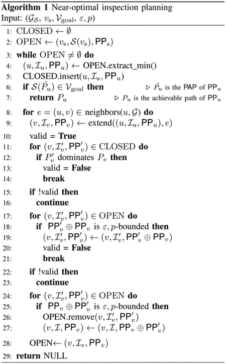
To compute a near-optimal inspection path (Alg. 1 and Fig. 6), we extend each path considered by our search algorithm to be a path pair and use this additional data to prune away approximately-dominated paths. Similar to A*, our algorithm uses two priority queues OPEN and CLOSED to track the nodes considered by the search. It starts by inserting the start vertex $\left(v_{\text{s}},\mathcal{S}\left(v_{\text{s}}\right)\right)$ to the OPEN list together with the path pair PP_s = (P_s, P_s) (here P_s is a path containing only start vertex v_s) (line 2).

Fig. 6:

Visualization of Alg. 1 initialized with ε = 2/3 and p = 1/2 (only the relevant parts of the inspection graph are depicted). The search starts from (a, ∅) with the trivial PAP of length zero and no points inspected. (a) Two paths (red and blue) are extended from the start node to (b, {0}) and (c, {1}) with path pairs PP₁ and PP₂, respectively (the PAP’s of each path have the same length and coverage as the paths themselves). (b) Blue path extended to (d, {0}) with $\mathcal{l}\left(P_1\right)=\mathcal{l}\left({\tilde{P}}_1\right)=2$ and $\mathcal{S}\left(P_1\right)=S\left({\tilde{P}}_1\right)=\left\{0\right\}$. (c) Red path extended to (d, {1}) with $\mathcal{l}\left(P_2\right)=\mathcal{l}\left({\tilde{P}}_2\right)=3$ and $\mathcal{S}\left(P_2\right)=S\left({\tilde{P}}_2\right)=\left\{1\right\}$. Here, PP₁ ⊕ PP₂ ε, p-dominates PP₂ and the red path is discarded and PAP₁ is updated to have length 2 and coverage {0, 1} (d) Blue path extended to vertex (e, {0, 2}). Here, $\mathcal{l}\left(P_1\right)=\mathcal{l}\left({\tilde{P}}_1\right)=3$ and $\mathcal{S}\left(P_1\right)=\left\{0,2\right\}$, $S\left({\tilde{P}}_1\right)=\{0,1,2\}$. The algorithm terminates with the path a − b − d − e whose length is 3 and has coverage of {0, 2}. Notice that the path a−c−d−e (not computed) is optimal as its length is four and it has complete coverage. The computed path is within the bounds ensured by the approximation factor p and ε.

Our algorithm proceeds in a similar fashion to A*—we pop the most promising node n = (u, ${\mathcal{I}}_u$, PP_u) from OPEN (line 4) and move it to CLOSED (line 5). If the PAP of this node is in the goal set ${\mathcal{V}}_{\text{goal}}$ (line 6), we terminate the search and return the achievable path of PP_u (line 7). If not, we consider all neighboring edges e of u in $\mathcal{G}$ and extend the node n (line 9). This is akin to computing n’s neighbors in ${\mathcal{G}}_{\mathcal{S}}$.

At this point our algorithm deviates from the standard A* algorithm. For each newly-created node (v, ${\mathcal{I}}_v$, PP_v) we check if there exists a node in CLOSED that dominates it. If so, this node is discarded (lines 11–14). If no such node exists in the CLOSED list, we check if there exists a node in OPEN that may subsume it. If so, that node is updated and this node is discarded (line 17–21). Finally, we check if this node can subsume nodes that are in OPEN. If so, such nodes are discarded and this node is updated. (line 24–27).

It is straightforward to see that (i) the first path pair is ε, p-bounded and hence by induction (ii) all path pairs in the search are ε, p-bounded. Furthermore, when the algorithm terminates, it has found a valid solution whose potentially-achievable path is in the goal set. This yields the following corollary:

Corollary 1:

Alg. 1 computes a path P that ε, p-dominates the optimal inspection path P*. Namely, that ℓ(P) ≤ (1+ε)·· ℓ(P*) and $\left|\mathcal{S}(P)\right|\ge p\cdot \left|\mathcal{S}(P)\cup \mathcal{S}\left(P*\right)\right|$.

C. Tightening approximation factors

Recall that our algorithm starts with approximation parameters p₀ and ε₀. We endow our algorithm with a tightening factor f ∈ (0, 1], and at the i’th iteration we set our approximation parameters as p_i = p_i−1 + f ·· (1 − p_i−1) and ε_i = ε_i−1 + f ·· (0 − ε_i−1). As we will see (Sec. VI), the tightening allows our method to achieve asymptotic optimality.

D. Implementation details

1). Lazy computation in graph inspection planning:

We run our search algorithm on $\mathcal{G}$ (Alg. 1) without checking if its edges are collision free or not (recall that only the edges of $\mathcal{T}$ were explicitly checked for collision). Once a solution is found, we start checking edges one by one until the entire path was found to be collision free or until one edge is found to be in collision, in which case we remove it from the edge set. This approach is common to speed up motion-planning algorithms when edges are expensive to evaluate [12, 21].

2). Node extension in graph inspection planning:

Any optimal inspection path can be decomposed into a sequence of vertices that improve the coverage of the path called milestones. It is straightforward to see that an optimal inspection path will (i) terminate at a milestone and (ii) connect a pair of milestones via a shortest path in $\mathcal{G}$. Following this observation, instead of extending each path P from a vertex u by all outgoing edges in $\mathcal{G}$ (Alg. 1, line 8), we run a Dijkstra-like search from u and collect all first-met vertices that can be milestones.

3). Heuristic computation in graph inspection planning:

Recall that A* orders nodes in the OPEN list according to their computed cost-to-come added to a heuristic estimate of their cost to reach the goal. The heuristic function that we use for vertex $\left(u,{\mathcal{I}}_u\right)$ is computed as follows: we run a Dijkstra search on $\mathcal{G}$ from u and consider the vertices ${\mathcal{V}}_u$ encountered during the search. We terminate when $\left({\cup }_{v\in {\mathcal{V}}_u}\mathcal{S}(v)\right)\cup {\mathcal{I}}_u={\mathcal{I}}_G$ and use the maximal distance between u to any node in ${\mathcal{V}}_u$ as our admissible [23] heuristic function.

VI. THEORETICAL GUARANTEES

We provide a proof sketch showing that, asymptotically, the length and coverage of the path produced by IRIS will converge to the length and coverage of an optimal inspection path. For ease of exposition, we state our results for the following simplified variant of IRIS where we start with an empty roadmap G₀ and some initial approximation factors ε₀ and p₀. At each iteration i we (i) sample a collision-free configuration q_i uniformly at random from $\mathcal{X}$, (ii) add q_i to roadmap G_i and connect it to all samples within radius r_i, and (iii) compute a near-optimal inspection path on this roadmap with parameters ε_i and p_i. (Namely, instead of implicitly constructing an RRG, we implicitly construct a PRM. While not identical, both roadmaps exhibit similar properties which are typically easier to show for PRMs.)

Roughly speaking, the connection radius r_i was chosen to ensure that as i → ∞ an optimal inspection path may be traced arbitrarily well by the roadmap ${\left\{G_i\right\}}_{i=1}^{\infty }$. The approximation factors were chosen such that ε_i > ε_i+1, p_i < p_i+1, $\underset{i\to \infty }{\text{lim}}{\epsilon }_i=0$ and $\underset{i\to \infty }{\text{lim}}{p}_i=1$. This will ensure that as i → ∞ the inspection path found will converge to an optimal inspection path in G_i.

A key result that we rely on is probabilistic exhaustivity (see, [49, Thm. IV.5] and [25, 51]). Roughly speaking, it is the notion that given a sufficiently large set of uniformly sampled configurations, any path can be traced arbitrarily well.

Finally, we assume that for every configuration along an optimal inspection path, there exists a neighborhood of configurations that share the same visibility. This is critical as we will not be able to exactly trace an optimal inspection path but only to iteratively approximate it. When this assumption holds we say that our inspection problem is well behaved.

The combination of (i) probabilistic exhaustivity, (ii) the ε, p-dominance of our graph inspection algorithm (Cor. 1) (iii) that $\underset{i\to \infty }{\text{lim}}{\epsilon }_i=0$ and $\underset{i\to \infty }{\text{lim}}{p}_i=1$, and (iv) that our inspection problem is well behaved ensures that asymptotically, our algorithm will converge to an optimal inspection path.

VII. RESULTS

We evaluated IRIS on two simulated scenarios: (1) a planar manipulator inspecting the boundary of a square region (Fig. 7a) and (2) a CRISP robot inspecting the inner surface of a pleural cavity (Fig. 7b). All tests were run on a 3.4GHz 8-core Intel Xeon E5–1680 CPU with 64GB of RAM.

Fig. 7:

Simulation scenarios. (a) A 5-link planar manipulator (orange) inspects the boundary of a square region (blue) where rectangular obstacles (red) may block the robot and occlude the sensor. The sensor’s field of view (FOV) is represented by the yellow region. $\mathcal{S}(q)$ are the points on the boundary in the sensor’s unobstructed FOV, and are shown in purple. (b) The pleural effusion inspection scenario involves the CRISP robot (orange) inspecting the inner surface of a pleural cavity, including the POI that are covered (green) and non-covered (blue) from the current robot configuration.

A. Planar manipulator scenario

In this scenario, depicted in Fig. 7a, we have a 5-link planar manipulator fixed at its base that is tasked with inspecting the boundary of a rectangular 2D workspace. We start by evaluating IRIS for fixed p and ε and then compare it with RRTOT using our approach for dynamically reducing the approximation factors. For every set of parameters we ran ten experiments for 1000 seconds and report the average value together with the standard deviation.

When p = 1 and we vary ε (Fig. 8a), we can see that even small approximation factors (e.g., ε = 0.5) allow to dramatically increase the coverage obtained as each search episode takes less time and more configurations can be added to the RRT tree. While using ε = 0 did not result in 80% coverage even after 1000 seconds, this was achieved within one second for ε ≥ 1.0. This comes at the price of slightly longer inspection paths. When ε = 0 and we vary p (Fig. 8b), we get roughly the same coverage per time but at the price of much longer paths for higher values of p.

Fig. 8:

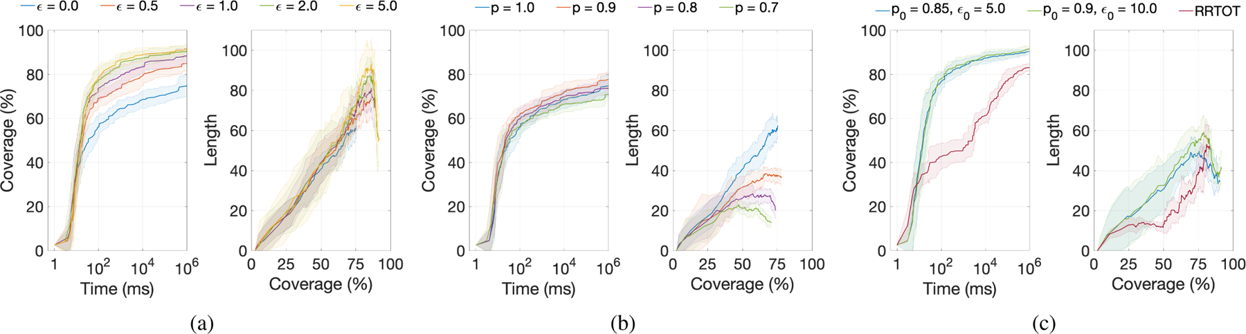
Quality of inspection paths computed for the planar manipulator. (a) IRIS running with p = 1, f = 0 and varying values of ε. (b) IRIS running with ε = 0, f = 0 and varying values of p. (c) Comparison of IRIS and RRTOT. IRIS running with two input parameter settings, both with f = 0.03.

Following the above discussion, when reaching high coverage is the sole objective, one should use large initial values of p₀ and ε₀. When we want initial solutions to also be short, one should start with smaller approximation factors. We compared IRIS with different initial approximation factors to RRTOT [6] (Fig. 8c). We can see that our approach allows to produce higher-quality paths than RRTOT. For example, IRIS obtains more than a 2450× speedup when compared to RRTOT when producing the same quality of inspection planning for the case of roughly 83% coverage and path length of 53 units. Final inspection paths obtained by IRIS are both shorter and inspect larger portions of $\mathcal{I}$.

B. Pleural effusion scenario for the CRISP robot

The anatomical pleural effusion environment for this simulation scenario was obtained from a Computed Tomography (CT) scan of a real patient suffering from this condition, and a fine discretization of the internal surface of the pleural cavity is used as the set of POI. We also use the internal surface of the cavity as obstacles, and prohibit the robot from colliding with the pleural surface, lung, and chest wall (except at tube entry points). Pleural effusion volumes can be geometrically complex, as the way in which the lung separates from the chest wall can be inconsistent. This results in unseparated regions of the lung’s surface that can inhibit movement and occlude the sensor from visualizing areas further in the volume.

Here we consider a CRISP robot with two tubes, where a snare tube is grasping a camera tube in order to create a parallel structure made of thin, flexible tubes. Each tube can be independently rotated in three dimensions about its entry point into the body, and independently translated into and out of the cavity. The system has 8 degrees of freedom with a configuration space of $\mathcal{S}\mathcal{O}{(3)}^2\times {ℝ}^2$, which enables the parallel structure to move in a manner that enables obstacle avoidance as well as precise control of the camera’s pose.

We ran IRIS and RRTOT for this scenario ten different times for 10,000 seconds (Fig. 9). Similar to the planar manipulator scenario, IRIS allows to produce higher-quality paths than RRTOT. For example, IRIS obtains more than a 25× speedup when compared to RRTOT when producing the same quality of inspection planning for the case of roughly 32% coverage and path length of 1.2 units.

Fig. 9:

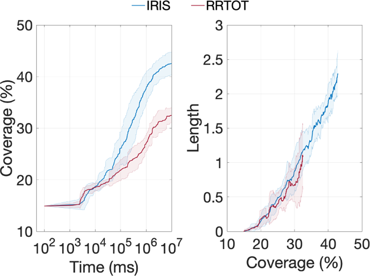
Comparing quality of inspection paths computed for the pleural effusion scenario. IRIS was run with p₀ = 0.8, ε₀ = 10, and f = 0.01.

VIII. CONCLUSION AND FUTURE WORK

In this work we presented IRIS, an algorithmic framework for computing asymptotically-optimal inspection plans. Our key contribution is an algorithm to efficiently compute near-optimal inspection plans on graphs. We showed IRIS outperforms the prior state-of-the-art, including in a medical application in which a surgical robot inspects a tissue surface inside the body as part of a diagnostic procedure.

We now highlight several avenues for further improving the IRIS framework. The first is accounting for dynamic updates in graph inspection planning. In future versions we would like to reuse information from previous search episodes. We suggest to adapt relevant methods from the graph-search literature (e.g., [18, 44, 30]). The second avenue is to efficiently sample configurations in RRT construction. Currently, in our RRT constructions we sample configurations uniformly at random from $\mathcal{X}$. Similar to goal bias commonly implemented in RRT, we suggest to bias sampling towards configurations that increase coverage. The third avenue is to explore the influence of hyper-parameters p and ϵ and optimize them. The fourth avenue is to parallelize graph building (including edge validation) and graph searching.

REFERENCES

- [1].Almadhoun Randa, Taha Tarek, Seneviratne Lakmal, Dias Jorge, and Cai Guowei. A survey on inspecting structures using robotic systems. Int. J. Advanced Robotic Systems, 13(6), 2016. [Google Scholar]
- [2].Anderson Patrick L., Mahoney Arthur W., and Webster Robert J. III. Continuum Reconfigurable Parallel Robots for Surgery: Shape Sensing and State Estimation With Uncertainty. IEEE Robotics and Automation Letters, 2 (3):1617–1624, 2017. [DOI] [PMC free article] [PubMed] [Google Scholar]
- [3].Bingham Brian, Foley Brendan, Singh Hanumant, Camilli Richard, Delaporta Katerina, Eustice Ryan, Mallios Angelos, Mindell David, Roman Christopher, and Sakellariou Dimitris. Robotic Tools for Deep Water Archaeology: Surveying an Ancient Shipwreck with an Autonomous Underwater Vehicle. J. of Field Robotics, 27(6):702–717, 2010. [Google Scholar]
- [4].Bircher Andreas, Alexis Kostas, Burri Michael, Oettershagen Philipp, Omari Sammy, Mantel Thomas, and Siegwart Roland. Structural Inspection Path Planning via Iterative Viewpoint Resampling with Application to Aerial Robotics In IEEE Int. Conf. Robotics and Automation (ICRA), pages 6423–6430. IEEE, 2015. [Google Scholar]
- [5].Bircher Andreas, Kamel Mina, Alexis Kostas, Burri Michael, Oettershagen Philipp, Omari Sammy, Mantel Thomas, and Siegwart Roland. Three-dimensional coverage path planning via viewpoint resampling and tour optimization for aerial robots. Autonomous Robots, 40 (6):1059–1078, 2016. [Google Scholar]
- [6].Bircher Andreas, Alexis Kostas, Schwesinger Ulrich, Omari Sammy, Burri Michael, and Siegwart Roland. An Incremental Samplingbased Approach to Inspection Planning: The Rapidlyexploring Random Tree Of Trees. Robotica, 35(6):1327–1340, 2017. [Google Scholar]
- [7].Bogaerts Boris, Sels Seppe, Vanlanduit Steve, and Penne Rudi. A Gradient-Based Inspection Path Optimization Approach. IEEE Robotics and Automation Letters, 3(3): 2646–2653, 2018. [Google Scholar]
- [8].Bohlin Robert and Kavraki Lydia E.. Path Planning Using Lazy PRM. In IEEE Int. Conf. Robotics and Automation (ICRA), pages 521–528, 2000. [Google Scholar]
- [9].Chen Peng and Nie Yu. Bicriterion shortest path problem with a general nonadditive cost. Transportation Research Part B: Methodological, 57:419–435, 2013. [Google Scholar]
- [10].Choset Howie M., Hutchinson Seth, Lynch Kevin M., Kantor George, Burgard Wolfram, Kavraki Lydia E., and Thrun Sebastian. Principles of Robot Motion: Theory, Algorithms, and Implementation. MIT press, 2005. [Google Scholar]
- [11].Danner Tim and Kavraki Lydia E.. Randomized Planning for Short Inspection Paths. In IEEE Int. Conf. Robotics and Automation (ICRA), pages 971–976, 2000. [Google Scholar]
- [12].Dellin Christopher M. and Srinivasa Siddhartha S.. A Unifying Formalism for Shortest Path Problems with Expensive Edge Evaluations via Lazy Best-First Search over Paths with Edge Selectors. In Int. Conf. Automated Planning and Scheduling (ICAPS), pages 459–467, 2016. [Google Scholar]
- [13].Dijkstra Edsger W.. A Note on Two Problems in Connexion with Graphs. Numerische Mathematik, 1(1): 269–271, 1959. [Google Scholar]
- [14].Edelkamp Stefan, Pomarlan Mihai, and Plaku Erion. Multiregion Inspection by Combining Clustered Traveling Salesman Tours With Sampling-Based Motion Planning. IEEE Robotics and Automation Letters, 2(2):428–435, 2017. [Google Scholar]
- [15].Ehrgott Matthias and Gandibleux Xavier. A survey and annotated bibliography of multiobjective combinatorial optimization. OR-Spektrum, 22(4):425–460, 2000. [Google Scholar]
- [16].Englot Brendan and Hover Franz S.. Sampling-Based Coverage Path Planning for Inspection of Complex Structures. In Int. Conf. Automated Planning and Scheduling (ICAPS), pages 29–37, 2012. [Google Scholar]
- [17].Englot Brendan J. and Hover Franz S.. Planning Complex Inspection Tasks Using Redundant Roadmaps. In Int. Symp. Robotics Research (ISRR), pages 327–343, 2011. [Google Scholar]
- [18].Frigioni Daniele, Marchetti-Spaccamela Alberto, and Nanni Umberto. Fully Dynamic Algorithms for Maintaining Shortest Paths Trees. J. Algorithms, 34(2):251–281, 2000. [Google Scholar]
- [19].Galceran Enric and Carreras Marc. A survey on coverage path planning for robotics. Robotics and Autonomous Systems, 61(12):1258–1276, 2013. [Google Scholar]
- [20].Gracias Nuno, Ridao Pere, Garcia Rafael, Escartín Javier, L’Hour Michel, Cibecchini Franca, Campos Ricard, Carreras Marc, Ribas David, Palomeras Narcís, et al. Mapping the Moon: Using a lightweight AUV to survey the site of the 17th Century ship La Lune In OCEANS-Bergen, 2013 MTS/IEEE, pages 1–8. IEEE, 2013. [Google Scholar]
- [21].Haghtalab Nika, Mackenzie Simon, Procaccia Ariel D., Salzman Oren, and Srinivasa Siddhartha S.. The Provable Virtue of Laziness in Motion Planning. In Int. Conf. Automated Planning and Scheduling (ICAPS), pages 106–113, 2018. [Google Scholar]
- [22].Halperin Dan, Salzman Oren, and Sharir Micha. Algorithmic motion planning In Handbook of Discrete and Computational Geometry, Third Edition, pages 1311–1342. CRC Press LLC, 2018. [Google Scholar]
- [23].Hart Peter E., Nilsson Nils J., and Raphael Bertram. A Formal Basis for the Heuristic Determination of Minimum Cost Paths. IEEE Transactions on Systems, Science, and Cybernetics, 4(2):100–107, 1968. [Google Scholar]
- [24].Hauser Kris. Lazy collision checking in asymptoticallyoptimal motion planning. In IEEE Int. Conf. Robotics and Automation (ICRA), pages 2951–2957, 2015. [Google Scholar]
- [25].Ichter Brian, Schmerling Edward, and Pavone Marco. Group Marching Tree: Sampling-Based Approximately Optimal Motion Planning on GPUs. In IEEE Int. Conf. Robotic Computing (IRC), pages 219–226, 2017. [Google Scholar]
- [26].Matthew Johnson-Roberson Oscar Pizarro, Williams Stefan B., and Mahon Ian. Generation and Visualization of Large-Scale Three-Dimensional Reconstructions from Underwater Robotic Surveys. J. of Field Robotics, 27(1): 21–51, 2010. [Google Scholar]
- [27].Kafka Přemysl, Faigl Jan, and Váňa Petr. Random Inspection Tree Algorithm in Visual Inspection with a Realistic Sensing Model and Differential Constraints. In IEEE Int. Conf. Robotics and Automation (ICRA), pages 2782–2787, 2016. [Google Scholar]
- [28].Karaman Sertac and Frazzoli Emilio. Sampling-Based Algorithms for Optimal Motion Planning. Int. J. Robotics Research (IJRR), 30(7):846–894, 2011. [Google Scholar]
- [29].Kavraki Lydia E., Svestka Petr, Latombe Jean-Claude, and Overmars Mark H.. Probabilistic roadmaps for path planning in high dimensional configuration spaces. IEEE Trans. Robotics and Automation, 12(4):566–580, August 1996. [Google Scholar]
- [30].Koenig Sven, Likhachev Maxim, and Furcy David. Lifelong Planning A*. Artificial Intelligence, 155(1–2):93–146, 2004. [Google Scholar]
- [31].Kuffner James J. and LaValle Steven M.. RRT-Connect: An Efficient Approach to Single-Query Path Planning. In IEEE Int. Conf. Robotics and Automation (ICRA), volume 2, pages 995–1001, 2000. [Google Scholar]
- [32].Kuntz Alan, Bowen Chris, Baykal Cenk, Mahoney Arthur W., Anderson Patrick L., Maldonado Fabien, Webster Robert J. III, and Alterovitz Ron. Kinematic Design Optimization of a Parallel Surgical Robot to Maximize Anatomical Visibility via Motion Planning. In IEEE Int. Conf. Robotics and Automation (ICRA), pages 926–933, 2018. [Google Scholar]
- [33].Latombe Jean-Claude. Robot Motion Planning. Kluwer, Boston, MA, 1991. [Google Scholar]
- [34].LaValle Steven M.. Planning Algorithms. Cambridge University Press, Cambridge, U.K., 2006. [Google Scholar]
- [35].LaValle Steven M. and Kuffner James J.. Randomized Kinodynamic Planning. Int. J. Robotics Research (IJRR), 20(5):378–400, May 2001. [Google Scholar]
- [36].Li Yanbo, Littlefield Zakary, and Bekris Kostas E.. Asymptotically optimal sampling-based kinodynamic planning. Int. J. Robotics Research (IJRR), 35(5):528–564, 2016. [Google Scholar]
- [37].Lynch Kevin M. and Park Frank C.. Modern Robotics: Mechanics, Planning, and Control. Cambridge University Press, 2017. [Google Scholar]
- [38].Mahoney Arthur W., Anderson Patrick L., Swaney Philip J., Maldonado Fabien, and Webster Robert J. III. Reconfigurable Parallel Continuum Robots for Incisionless Surgery. In IEEE/RSJ Int. Conf. Intelligent Robots and Systems (IROS), pages 4330–4336, 2016. [Google Scholar]
- [39].Marble James D. and Bekris Kostas E.. Asymptotically near-optimal is good enough for motion planning. In Int. Symp. Robotics Research (ISRR), pages 419–436, 2011. [Google Scholar]
- [40].Niyaz Sherdil, Kuntz Alan, Salzman Oren, Alterovitz Ron, and Srinivasa Siddhartha. Following Surgical Trajectories with Concentric Tube Robots via Nearest-Neighbor Graphs. In Int. Symp. Experimental Robotics (ISER), 2018. [Google Scholar]
- [41].Papadopoulos Georgios, Kurniawati Hanna, and Patrikalakis Nicholas M. Asymptotically Optimal Inspection Planning using Systems with Differential Constraints In IEEE Int. Conf. Robotics and Automation (ICRA), pages 4126–4133. IEEE, 2013. [Google Scholar]
- [42].Pardalos Panos M., Migdalas Athanasios, and Pitsoulis Leonidas. Pareto optimality, game theory and equilibria, volume 17 Springer Science & Business Media, 2008. [Google Scholar]
- [43].Raffaeli Roberto, Mengoni Maura, Germani Michele, and Mandorli Ferruccio. Off-line view planning for the inspection of mechanical parts. International Journal on Interactive Design and Manufacturing (IJIDeM), 7(1): 1–12, 2013. [Google Scholar]
- [44].Ramalingam Ganesan and Reps Thomas. On the Computational Complexity of Dynamic Graph Problems. Theor. Comput. Sci, 158(1&2):233–277, 1996. [Google Scholar]
- [45].Line Blander Reinhardt and David Pisinger. Multi-objective and multi-constrained non-additive shortest path problems. Computers & OR, 38(3):605–616, 2011. [Google Scholar]
- [46].Salzman Oren and Halperin Dan. Asymptotically-optimal Motion Planning using lower bounds on cost. In IEEE Int. Conf. Robotics and Automation (ICRA), pages 4167–4172, 2015. [Google Scholar]
- [47].Salzman Oren and Halperin Dan. Asymptotically Near-Optimal RRT for Fast, High-Quality Motion Planning. IEEE Trans. Robotics, 32(3):473–483, 2016. [Google Scholar]
- [48].Salzman Oren, Hou Brian, and Srinivasa Siddhartha. Efficient Motion Planning for Problems Lacking Optimal Substructure. In Int. Conf. Automated Planning and Scheduling (ICAPS), pages 531–539, 2017. [Google Scholar]
- [49].Schmerling Edward, Janson Lucas, and Pavone Marco. Optimal sampling-based motion planning under differential constraints: The driftless case. In IEEE Int. Conf. Robotics and Automation (ICRA), pages 2368–2375, 2015. [DOI] [PMC free article] [PubMed] [Google Scholar]
- [50].Solovey Kiril, Salzman Oren, and Halperin Dan. New perspective on sampling-based motion planning via random geometric graphs. Int. J. Robotics Research (IJRR), 37(10):1117– 1133, 2018. [Google Scholar]
- [51].Starek Joseph A., Gómez Javier V., Schmerling Edward, Janson Lucas, Moreno Luis, and Pavone Marco. An asymptotically-optimal sampling-based algorithm for Bidirectional motion planning. In IEEE/RSJ Int. Conf. Intelligent Robots and Systems (IROS), pages 2072–2078, 2015. [DOI] [PMC free article] [PubMed] [Google Scholar]
- [52].Tivey Maurice A., Bradley Albert, Yoerger Dana, Catanach Rodney, Duester Alan, Liberatore Steve, and Singh Hanu. Autonomous Underwater Vehicle Maps Seafloor. Eos, Transactions American Geophysical Union, 78(22): 229–230, 1997. [Google Scholar]
- [53].Tsaggouris George and Zaroliagis Christos D.. Non-additive Shortest Paths. In European Symposium on Algorithms (ESA), pages 822–834, 2004. [Google Scholar]
- [54].Tsaggouris George and Zaroliagis Christos D.. Multiobjective Optimization: Improved FPTAS for Shortest Paths and Non-linear Objectives with Applications. Theory of Computing Systems, 45(1):162–186, 2009. [Google Scholar]