Abstract
A motion-planning problem’s setup can drastically affect the quality of solutions returned by the planner. In this work we consider optimizing these setups, with a focus on doing so in a computationally-efficient fashion. Our approach interleaves optimization with motion planning, which allows us to consider the actual motions required of the robot. Similar prior work has treated the planner as a black box: our key insight is that opening this box in a simple-yet-effective manner enables a more efficient approach, by allowing us to bound the work done by the planner to optimizer-relevant computations. Finally, we apply our approach to a surgically-relevant motion-planning task, where our experiments validate our approach by more-efficiently optimizing the fixed insertion pose of a surgical robot.
I. INTRODUCTION
In this work, we approach optimizing the setups of motion-planning problems to maximize the utility of a given task. We define the “setup” of a planning problem as any parameters we have control over that must be set before the planner is invoked. This includes, for example, the kinematic design of the robot. Another example of problem setup is the fixed insertion pose of a surgical robot tasked with following a surgeon-provided path, where a poor insertion pose can severely hinder the robot’s ability to do so (Fig. 1).
Fig. 1.

Left: A concentric tube robot deployed with a fixed insertion pose through the sinus. A path R to cut using the robot’s end-effector, or tip, is shown in yellow. Right: The insertion pose T2 on the right is preferable. It enables the robot (depicted here as a planar manipulator) to follow the path R without colliding with obstacle .
This example demonstrates how a problem’s setup can dramatically affect the quality of solutions generated by a motion planner. However, selecting the best problem setup from a set of candidates is challenging. The motions required to complete a given task are naturally complex, as they must both avoid collisions in constrained areas and optimize some objective. This makes it difficult to evaluate the cost of motions required by a problem setup, and thus the quality of the setup, without the use of a motion planner itself.
We therefore apply an approach that interleaves optimization with motion planning to evaluate the quality of candidate problem setups. While we are not the first to do so [3], [4], [17], previous approaches treat the planner as a black box. Our key insight is that opening this black box enables a more computationally-efficient approach—namely by using the optimizer to restrict work done by the planner to only optimization-relevant computations. We present a simple-yet-effective implementation of this idea that resembles branch and bound [18].
Specifically, we use the optimizer to derive some bound for each candidate setup evaluated by the motion planner, where any setup with cost greater than will not affect the optimization process. Fittingly, many planners are able to derive a lower bound on the cost of their final solution before fully computing it. Should exceed , the planner can abort given that additional work would not affect the optimization. We also demonstrate how a planner can be modified to maximize this approach’s efficiency gains.
Our approach can be used to optimize the setups of various motion-planning problems, ranging from the placements of robots on a factory floor to the design space of a reconfigurable robot. In this paper we explore the surgical applications that motivated this work. Our surgical robot, a Concentric Tube Robot (CTR), enables new minimally-invasive surgeries in constrained areas due to its dexterity and small diameter [11]. Often these surgeries require the robot to follow with its tip some path R dictated by the surgeon, for example to cut a window in the skull during pituitary gland surgery (Fig. 1). With this in mind, we developed the Nearest-Neighbor Fréchet (NNF) planner in [21] that computes a CTR motion plan closely following such a path.
A key limitation of this planner is that it fails to consider the insertion pose T of the CTR, instead committing to one set arbitrarily. Unfortunately, the CTR’s unintuitive kinematics make it difficult for a human to perfectly discern the reachable workspace given an insertion pose, likely making the initial insertion pose sub-optimal. Our experiments support this by optimizing T, while also applying our approach to reduce convergence time by approximately 2×.
We begin with our approach to interleaving optimization with motion planning, which more-efficiently uses the planner to evaluate candidate problem setups (Sec. III). We then apply this approach to our specific surgical task (Sec. IV) and modify our NNF planner to maximize its computational efficiency (Sec. V). Finally, we discuss results in Sec. VI.
II. RELATED WORK
Optimizing the insertion pose of a CTR is similar to the problem of base placement for a mobile manipulator. Though approaches such as inverse reachability analysis [20], [26] have been applied to this problem, they do not account for the motions required by the specific task at hand. This is critical in our domain: while an entire path R may be reachable in the absence of obstacles, the interaction of the CTR’s kinematics with the highly-constrained environments of surgery drastically affects the planner’s ability to follow paths [21]. This induces a complex mapping from T to solution cost, requiring us to consider the actual motions required of the robot given T.
Our optimization of the CTR’s insertion pose is also similar to optimizing the placement of surgical ports, devices that provide entry vectors for drugs and medical tools. Feng et al. [9] optimize port placements for robotically-assisted cholecystectomy, while Hayashi et al. [13] do so for laparoscopic gastrectomy. While these approaches reason spatially about the relationship between port placement and reachable regions of the anatomy, they do not account for the series of motions required during their respective procedures.
Yet another similar problem involves motion planning with steerable needles, where the needle’s insertion into the patient can drastically affect the set of locations reachable by its tip [2], [15]. However, a distinction must be drawn between CTRs and steerable needles. A CTR can reasonably be approximated as having holonomic kinematics similar to a serial-link manipulator, where each DOF of the robot can be controlled independently [24]. By contrast, a steerable needle is a nonholonomic system more similar in control to a wheeled vehicle than a traditional manipulator.
Some prior CTR-specific works have focused on optimizing the kinematic design of the robot to avoid obstacles while reaching a set of target points [5] or maximizing coverage of a volume [6]. Much like inverse reachability analysis, these geometric approaches consider only the ability to reach placements of the robot’s tip, rather than the motions required to complete a task. They thus refrain from using a motion planner in the optimization process, which hinders their applicability to highly-constrained tasks. This is especially true in our domain, where the CTR is required to follow an entire path with its tip rather than reaching disjoint points.
The prior works most similar to ours come from Baykal et al. [3], [4] and Kuntz et al. [17]. These approaches use Adaptive Simulated Annealing (ASA) [19] to optimize the kinematic designs of surgical robots, together with a motion planner to evaluate the quality of candidate designs. They thus account for the series of motions needed to complete their respective tasks. The former work seeks to optimize the design of piece-wise cylindrical robots in order to reach a set of target points. The latter aims to optimize the design of a parallel, needle-diameter surgical robot for the purpose of inspection planning [1]. In addition to having different motion-planning tasks from our work, these approaches do not use the optimizer to bound the work done by the planner.
III. EFFICIENT SETUP EVALUATION
In our approach of interleaving optimization and motion planning, we focus on the use of gradient-free optimizers [19], [23]. We do so because it is unclear how to derive the closed-form gradient of solution cost with respect to problem-setup parameters for many motion planners, including our NNF planner.
Almost all gradient-free optimizers operate by sampling a state x, evaluating its fitness (or quality) via some function E(x), and then using this value in a comparison that informs the optimizer’s actions. In our case x is a candidate problem setup and E(x) is the cost returned by invoking a motion planner given that problem setup. With our specific surgical application, this would then make x a candidate insertion pose T and E(x) the corresponding cost returned by NNF. As we will demonstrate, this cost captures the deviation of the CTR’s tip from the dictated path.
We focus our analysis in this section primarily on fitness evaluations and their subsequent comparisons. Specifically, we consider Adaptive Simulated Annealing [19] (ASA), an asymptotically-optimal gradient-free optimizer that makes minimal assumptions about the topology of the space. (We briefly discuss other optimizers at the end of this section.) At each iteration, ASA samples u ∈ [0,1] and a new problem setup x, then computes the setup’s fitness E(x). It “accepts” the new setup if:
| (1) |
Here, e′ is the fitness of the most recently accepted setup and K is the temperature, a parameter that decays exponentially as ASA progresses. While ASA may accept an inferior setup with some probability in order to escape local minima, the likelihood that it will accept x decreases as E(x) increases. That is, the worse a setup, the less likely the optimizer is to utilize it. This is characteristic of many gradient-free optimizers. In the case of ASA, we can show from (1) that no setup will be accepted with:
| (2) |
We note that the value of this bound, which we denote , changes each iteration of ASA as a function of u, K, and e′. Such a bound is useful given that many motion planners are able to lower-bound the cost of their final solution before they have finished computing it. Consider, for example, a search-based planner that finds the shortest path on a graph using the algorithm Dijkstra [8]. At each iteration the algorithm removes (or “expands”) a node from its priority queue, the distance (or “cost-to-come”) value of which lower-bounds the cost of the final path.
In our approach, this property can be used to derive a straightforward abort strategy similar to branch and bound [18]. In addition to passing a problem setup x to the planner for evaluation, ASA also computes and passes the current bound from (2). As the planner works to generate a solution and its fitness E(x), it also updates a lower bound on the solution’s final cost. Should exceed , the candidate setup x is guaranteed not be to accepted. The planner should then abort immediately to prevent unnecessary computation (Fig. 2).
Fig. 2.
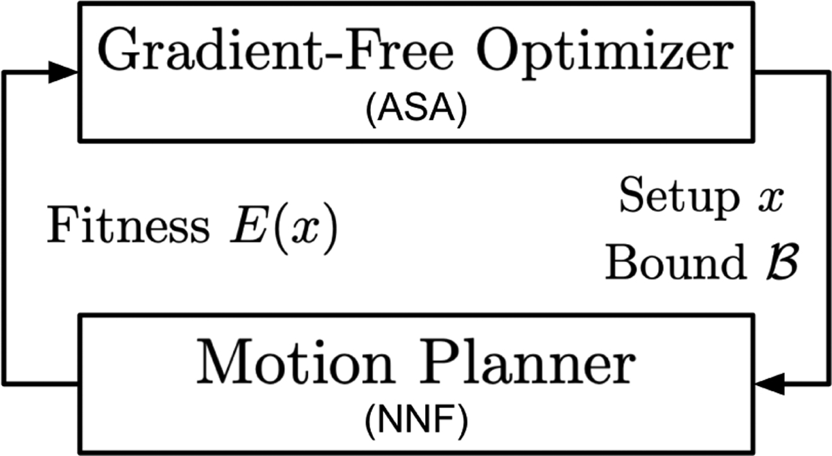
An overview of our approach. In addition to sending a problem setup x to the planner for evaluation, the optimizer also sends a bound . Once this cost is exceeded, further evaluation by the planner will not change the steps taken by the optimizer. We note that in our specific application, ASA is used as the optimizer and NNF as the planner.
Another Optimizer:
While we have performed this analysis for ASA, we note that similar bounds can be derived for many other gradient-free optimizers, making our abort strategy a general one. For example, consider cross-entropy minimization (CEM) [23], which on each iteration i) samples n problem setups from distribution , ii) evaluates E(xi) for each sampled xi, and iii) picks the k best setups and refits to them. The bound when evaluating some E(xi) is the fitness of the kth best setup evaluated so far on that iteration, given that a sampled setup with worse fitness is guaranteed not to affect .
IV. SURGICAL APPLICATION
In the previous section we laid out a general approach for efficiently interleaving optimization with motion planning. We now apply this approach to our specific problem domain: following a path R specified by a human using the tip of a highly-dexterous surgical tool known as a Concentric Tube Robot [11], or CTR (Fig. 3). We begin with key definitions and then detail our planner for this task, NNF, which we proceed to use as the bottom half of Fig. 2 to optimize the insertion pose T of the robot.
Fig. 3.
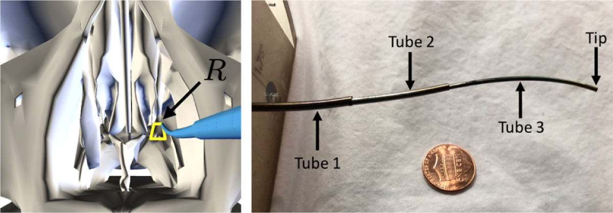
Left: A CTR (blue) follows a reference path R (yellow) with its tip to cut a window through the skull in simulation. Right: A three-tube CTR alongside a coin for scale. Because each tube rotates and translates, this particular CTR has 6-DOF.
A. Fundamental Definitions
We take as input a surgeon-specified reference path R. We represent this path as an ordered set of waypoints r0,…,rn in task-space, defined as the position of the CTR’s tip. Formally, R is encoded as a one-dimensional graph (VR, ER) in which directed edges connect subsequent waypoints (Fig. 4). We note that while our task-space definition is adequate for cutting with heat or a laser, our approach can trivially be used with other task-space definitions that account for the tip’s orientation, such as SE(3).
Fig. 4.
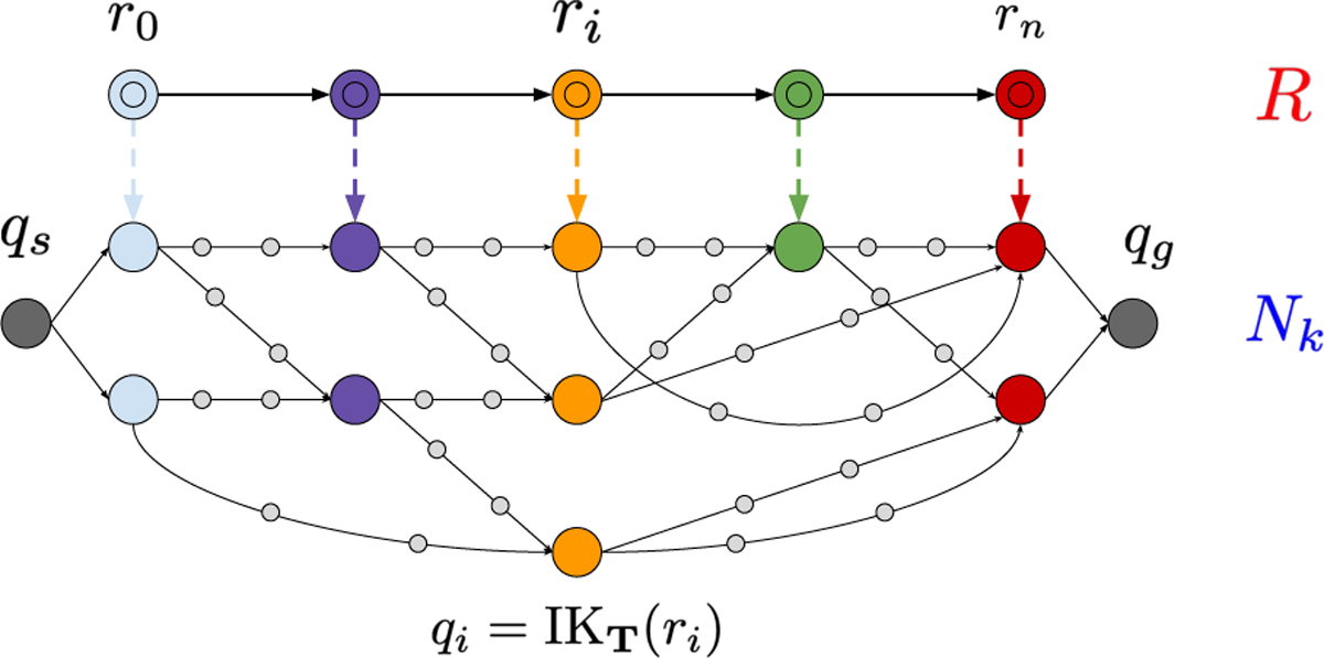
NNF constructs a graph Nk in configuration-space to follow a reference path R in task-space. Note that a single waypoint ri ∈ R may have multiple IKT solutions sampled. In this example IKT solutions are connected by j = 2 interpolated configurations, represented as grey nodes.
While our reference path R is given in task-space, execution on the robot requires a collision-free path in the configuration-space (the space of all possible configurations of the robot), also known as a motion plan. Each configuration qi is a d-dimensional point uniquely defining the robot’s shape, and thus must encode the translation and rotation of each of its tubes (Fig. 3). Therefore, for a CTR composed of t tubes .
We use the forward kinematics (FKT) operator to map points and paths in to points and paths in task-space, and the inverse kinematics (IKT) operator to map a point in task-space to one or more points, or “solutions”, in . Thus:
| (3) |
We denote the set of collision-free paths in as ΓT, and note that all of FKT, IKT, and ΓT depend on the insertion pose T of the CTR.
Taking our task into account, our motion plan in should follow R closely using the robot’s tip. To quantify this notion of how “closely” the tip’s path follows R, we use a well-studied measure of deviation or error between two paths known as the Fréchet distance [27]. While following R perfectly may not always be feasible, our planner should minimize this error as much as possible.
The Fréchet metric can be explained intuitively via an analogy, wherein a dog on a leash traverses one path with speed parameterization α as its owner traverses the other with parameterization β. (We note that α and β are independent.) Here, the Fréchet distance is the shortest leash length required for the dog and its owner to stay connected, assuming the two are moving optimally. Thus, the metric accounts for not only the relative positions of points on each path, but also the order in which those points are traversed. This ability to capture the “flow” of the two paths makes the metric a natural choice to measure error in our domain, as it allows a user to specify tasks such as tissue manipulation where the direction of motion matters.
B. Algorithmic Background
Given these definitions and a preset insertion pose T, our original NNF planner [21] minimizes:
| (4) |
where is the discrete Fréchet distance. We use this approximation, where the “leash” between the two paths is computed only for a discrete set of points, because computing the continuous Fréchet is computationally challenging [25].
The NNF planner approaches this objective by building a graph in (Fig. 4). To do so, n IKT solutions are randomly sampled for points on R, and each is connected to its k nearest-neighbors in . Rather than connecting two samples q1 and q2 directly with an edge, we add a path of j configurations interpolated between them. Nk also contains start and goal nodes qs and qg connected to IKT solutions for r0 and rn, the first and final waypoints on R, respectively. Note that the edges of Nk are directed and constrained to monotonically follow R.
Once Nk has been sampled, NNF applies the approach of Holladay et al. [14] to find a path γ ∈ Nk minimizing . In doing so, it constructs a directed tensor-product graph Φ = (VΦ, EΦ). VΦ contains one node (r, q) for every possible combination of a node r ∈ VR and a node . Each node (rx, qx) has an out-edge to:
| (5) |
Less formally, (rx, qx) has out-edges to all nodes that represent taking a “step” on the reference path R from rx, on the sampled graph Nk from qx, or both. Finally, the weight of an edge (rx, qx) → (ry, qy) is:
| (6) |
where is the Euclidean distance.
After constructing Φ, NNF searches it for the minimal-bottleneck path τ from (r0, qs) to (rn, qg), i.e. the path with the lowest possible maximum edge weight. We note that this path can be computed simply by applying a modified shortest-path algorithm, such as Dijkstra, that uses a max operator instead of addition to combine the distance value of a node with the weight of an outgoing edge. By extracting qi from each node (ri, qi) ∈ τ, we can then recover the path γ on Nk minimizing , where the bottleneck cost of τ (the weight of its heaviest edge) is the objective value [14]. The interpolated nodes of Nk better enable this value to approximate the true, continuous Fréchet [14].
C. Problem Statement
In our previous work with NNF [21], T was (arbitrarily) set and the problem called for optimizing (4). However, this initial pose is likely sub-optimal given the highly-constrained anatomy and the unintuitive, nonlinear kinematics of the CTR. Thus, we expand our problem statement by both optimizing the insertion pose T and generating a corresponding motion plan γ for this pose. Formally, our optimization problem is now:
| (7) |
To do this, we apply our approach to optimizing the problem setup detailed in Fig. 2. ASA is applied over SE(3), the space of insertion poses. During this process NNF is used to evaluate the fitness of each candidate pose, done by returning the value of the objective in (4) after planning.
V. DESIGNING A LAZY MOTION PLANNER
A. Motivation
Using the NNF motion planner to evaluate the fitness of candidate problem setups (i.e. insertion poses) allows us to accurately account for the motions required to follow the path R under each one. We showed previously in Sec. III that we can utilize the bound from (2) in this process to limit the computation done by the planner in each evaluation: once this cost is exceeded, the planner should abort given that any additional work it performs is irrelevant to the optimizer.
Notably, motion planners can be redesigned to better take advantage of such a bound. A search-based planner operating on a graph , for example, should be made as lazy as possible: instead of incurring a large computational cost on initialization, the planner should defer expensive computations until the corresponding nodes and edges of are processed by the search. One example would be collision-checking edges of as the search discovers them, rather than removing all in-collision edges of before the search begins.
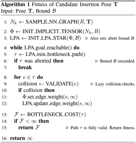
In this case, aborting the planner limits the set of processed nodes and thus naturally prunes many of these expensive computations. Given that NNF is one such search-based planner, we redesign it in a lazy fashion to increase the effectiveness of our bound. An outline of our lazy NNF implementation is given in Alg. 1.
B. Lazy Modifications
As is true of many motion planners, one of NNF’s largest overheads is collision-checking [21]. We recall that the planner searches for a path by first computing a minimal-bottleneck path τ on the tensor-product graph Φ using a modified shortest-path algorithm. In order to validate an edge (rx, qx) → (ry, qy) of Φ, the edge qx → qy on must be collision-checked. To perform these checks lazily [12], we apply the approach of Dellin and Srinivasa [7]. The planner performs no collision-checks initially and assumes that all edges of Φ are valid. The minimal-bottleneck path τ is then generated, the edges of which are validated until either i) the path is found to be completely free, or ii) some edge e ∈ τ is found to be in collision, at which point its weight is set to ∞. The search will then repeat and find the new minimal-bottleneck path given this weight change.
This process repeats until all paths are found to be in collision or a solution is found. Although this lazy approach limits collision-checks to edges that may be on the solution path, it also requires many reruns of the search given the frequent weight changes. Thus, rather than using Dijkstra as our search algorithm we use a bottleneck version of Lifelong Planning A* (LPA*) [16], which is able to reuse information from prior searches to accelerate future ones. We also memoize the results of collision-checking each edge qx → qy on to avoid repeat computation.
Another significant overhead NNF incurs is invoking FKT, required to define the weights of EΦ in (6). This is because computing FKT for a continuum robot such as the CTR requires modeling complex phenomena, such as elastic interactions between tubes [24]. In our original NNF implementation [21], Φ was constructed explicitly before the search was run. Not only did this use FKT to compute weights of edges never processed by the search, it required a large computational cost simply to initialize the planner.
To avoid this, our lazy NNF implementation represents Φ implicitly. An implicit representation only constructs nodes and edges of Φ when they are queried for by the search, with the exception of the start node (r0, qs). We note that given the definition of EΦ in (5), we can determine and construct the requested neighbors of any node (rx, qx) simply by inspecting those of rx ∈ VR (where R is given as input) and (where Nk is still constructed explicitly). Only then will FKT be invoked as in (6) to calculate the weights of the corresponding edges.
C. Aborting Evaluation
Having incorporated a large degree of laziness into our planner, we now utilize the bound . We compare the priority of each node expanded by bottleneck LPA* to , and abort further evaluation once it is exceeded. Since we do not use a heuristic, these priorities in LPA* are analogous to the distance values used in Dijkstra. The new lazy design of our planner makes this bound on the set of expanded nodes especially effective: fewer paths must be collision checked lazily, and fewer edges and nodes of Φ must be constructed. The latter in turn leads to fewer invocations of FKT.
Similar to Dijkstra, the priority of the node being expanded provides a lower bound on the cost of the minimal-bottleneck path τ ∈ Φ, and thus the objective representing the fitness of the candidate pose T [16]. Given that the priorities of expanded nodes are strictly non-decreasing over time [16], one can view this as initial optimism in which we assume an of zero (the priority of the start node), and slowly increase over time as Φ is constructed and edges are invalidated.
VI. EXPERIMENTS AND RESULTS
A. Experiment Design
We evaluate our approach in two scenarios inspired by minimally-invasive surgery of the pituitary gland, which is located adjacent to the brain. Each scenario requires the CTR to follow with its tip one of two paths located in the back of a human skull-base (Fig. 5). We foresee such paths being used to cut windows into the skull, thereby allowing the surgeon access to the pituitary gland.
Fig. 5.

We use two evaluation scenarios which require the robot to follow either Path A or B, depicted here inside the anatomy in yellow. Path A is more anterior and resides in less constrained anatomy, while Path B is further posterior and resides in more constrained anatomy. Each path is specified in the back of a human skull-base model (left, gray), into which the CTR (left, blue) is deployed.
Each scenario initializes ASA with a unique insertion pose T0, which is specified by a human familiar with the CTR’s kinematics. While both paths are kinematically reachable under their initial insertions, each presents a unique challenge. For Path A, T0 angles the base of the CTR in a manner that restricts its range of motion around certain portions of the path. Meanwhile, the initial insertion for Path B makes it impossible for the CTR to reach one of the path’s corners given obstacles.
Implementation Details:
For each path and initial insertion, we run ASA until convergence. We present metrics tied to computational efficiency and improvement in solution quality, all of which are averaged over 20 seeds. We set the parameters for NNF at empirically-chosen values intended to balance solution quality and runtime: n = 150 IKT samples, k = 10 nearest-neighbors, and j = 3 interpolated configurations. We use FCL [22] to perform collision-checks, and the kinematic model from [24] to perform FKT and IKT. All experiments were run on a 3.50GHz Intel Core i5 CPU with 16GB RAM.
B. Results and Discussion
Overall Results:
For both paths, we compare the Fréchet error returned by NNF using the initial insertion pose T0 and the best pose T* found by ASA (Fig. 6). We observe that in both cases T* corresponds to a significantly lower error than T0. This amounts to a decrease in average Fréchet error of 59.1% for Path A, and 65.9% for Path B. We depict T0 and T* for a particular seed with Path B in Fig. 9. We also demonstrate how T* enables the CTR to avoid obstacles and reach the previously infeasible corner with its tip.
Fig. 6.
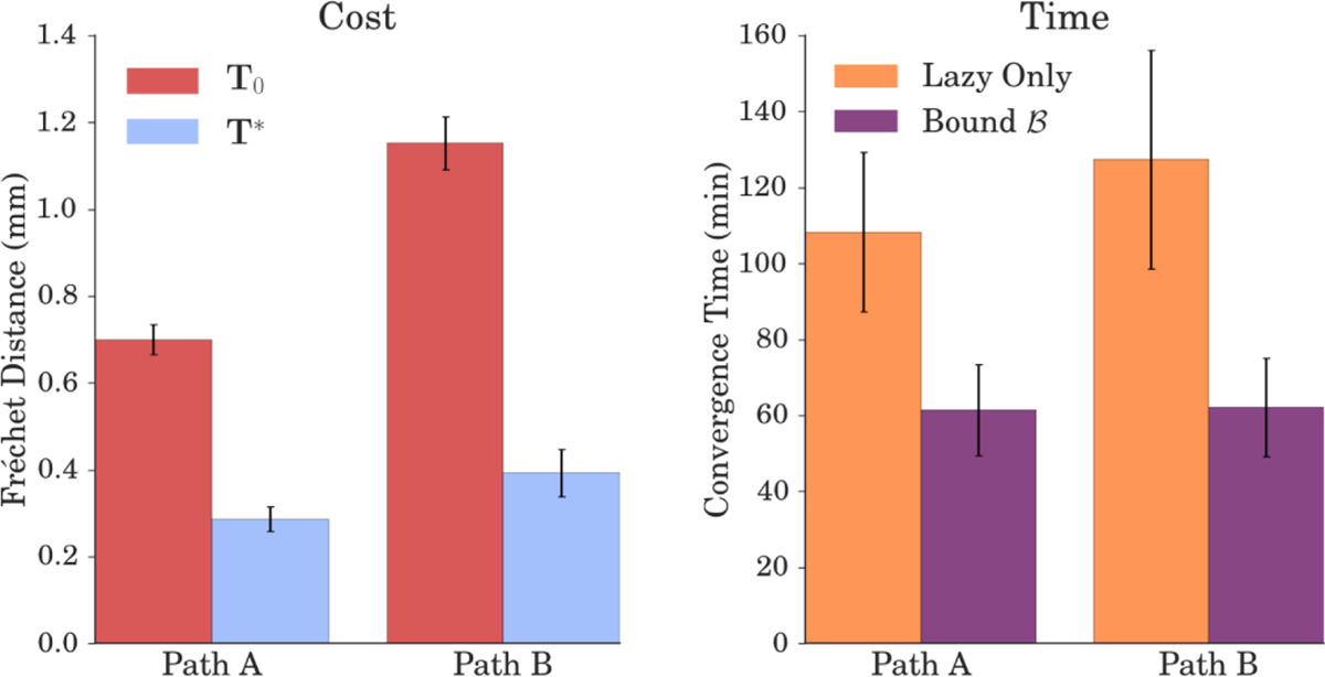
At left, we compare the costs for each path using the initial insertion pose T0 (red) and the final insertion pose T* (blue). At right, we report convergence times for each path with (purple) and without (orange) use of the bound .
Fig. 9.
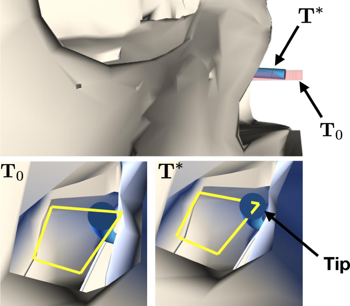
We depict both the initial insertion pose T0 and the final insertion pose T* for a run using Path B. We note that under T0, the CTR’s tip is unable to reach the top-right corner of the path due to obstacles. However, T* enables the CTR to maneuver around these obstacles. This example is detailed further in our accompanying video.
To also evaluate the effectiveness of our bound (Fig. 2) at increasing computational efficiency, we compare convergence times of ASA for both paths with and without the use of this bound (Fig. 6). In both cases we use the lazy NNF implementation detailed in Sec. V. We see that our approach, which bounds the work done by the planner in evaluating each candidate pose, leads to a dramatic decrease in average convergence time for both paths. This amounts to a 43.2% drop in average time for Path A and a 51.2% drop for Path B.
Given its non-interactive timescale, this optimization would be done offline before the medical procedure itself. The utility of using multiple initializations in this process is demonstrated in Fig. 8, which reveals how the final Fréchet error ASA converges to can vary significantly between different random seeds for the optimizer and planner. Particularly with Path B, re-running the optimizer with several different initializations has the potential to dramatically improve the quality of paths planned for the procedure.
Fig. 8.
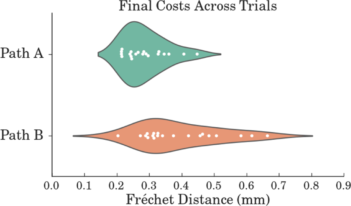
A violin plot of the final Fréchet errors ASA converged to over the 20 random seeds used for each path. Each white point represents the final error for a specific initialization, with the approximate distribution over errors shaded above and below each set of data. We note that T0 remained the same for each path between seed changes.
This need for multiple initializations makes it relatively easy to imagine scenarios where our dramatic speed-up is scaled across even lengthier and more expensive optimization problems. Other factors would also lengthen the timescales of these processes. Procedures will realistically be composed of multiple steps and thus require the CTR to follow a large set of paths rather than just one. Additionally, higher-valued planner parameters than ours will be needed for more challenging optimization problems and to produce truly optimal solutions.
Additional Metrics:
We report additional metrics tied to computational efficiency in Fig. 7. These results are discussed in the order they appear from left to right.
Fig. 7.
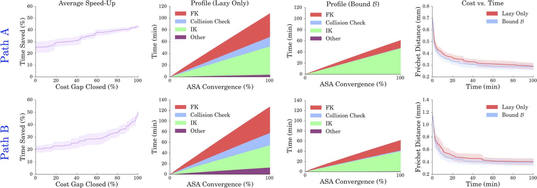
From left to right: i) The percentage of total time saved as a function of error improvement. ii) A profile of runtime for the optimization both without and with the bound used. iii) Fréchet as a function of time with and without .
We are interested not only in the overall time savings afforded by our bound , but also how the bound prunes computation as the optimization progresses. Towards this end, the first of these results correlates the average speed-up within each run with the error reduction accomplished by ASA. More technically, we report the percent reduction in compute time required for ASA to close a given percentage of the “cost gap” within each run. We define the cost gap as the difference in Fréchet error from T0 to T* : that is, the gap has been 0% closed when ASA evaluates the initial problem setup T0, and 100% closed when it evaluates the best setup T*. We note that ASA usually converges at a later point in time than when the cost gap is 100% closed.
Each path behaves differently in this regard. In the case of Path A, the portion of total time saved is roughly linear in the portion of error reduction that has been accomplished. However, the portion of total time saved with Path B increases at a higher rate when more of the cost gap is closed. By the time T* is discovered by ASA, runs using Path A save on average 43.1% of total compute time, while runs using Path B save on average 50.1%. Although convergence times vary, these results demonstrate that the average fraction of time saved to reach the best score remains fairly consistent.
Our next results profile the runtime of the ASA process to demonstrate the proportion of computation spent on various operations. We perform this profiling both without and with using the bound to reveal the sources of our efficiency gains. The runtime profiles for both paths are fairly similar, with collision-checks and FKT together constituting a majority of compute time. Given that our lazy NNF implementation makes the cost of these operations proportional to the number of nodes expanded by LPA*, aborting NNF using is very effective at reducing this cost and thus the overall runtime of the optimization. This is reflected in the profiling plots as well, where the only operation not flattened is IKT. This is logical, as constructing the graph Nk by sampling IKT solutions is an initialization cost of NNF.
Finally, we report Fréchet error as a function of runtime. We do so by averaging the lowest error found by each run within a given time budget. We see that ASA makes substantial gains early in the optimization, but displays a fairly long tail required to reach the best insertion pose T*. Notably, applying increases the rate of progress and dramatically shortens this tail.
VII. CONCLUSION AND FUTURE WORK
We present an approach to more-efficiently interleave optimization with motion planning by using the optimizer to place bounds on the work done by the planner. We then apply this approach to our specific use case of following surgical trajectories by optimizing the insertion pose of the robot. Finally, we present results in this domain that demonstrate significant improvements in computational efficiency.
One of the key limitations in this work is that we consider the parameters of our motion planner to be fixed during the optimization process. As such, one of our next goals is balancing our search over the space of insertion poses with a search over the space of NNF parameters. We intend to use our work in this paper as a fundamental building block in such a process, allowing us to use the motion planner more efficiently as its parameters are tuned.
Unlike the geometric approaches presented in [5] and [6], using NNF to evaluate the fitness of problem setups allows us to consider the motions required of the robot. However, these geometric methods are still less computationally-expensive than ours. Thus, we will explore integrating these less-costly approaches into ours to produce a hybrid approach. One example involves using these geometric approaches to reject candidate poses that would not place the entire path within the reachable task-space of the CTR given the anatomy.
Our approach in this work is straightforward albeit effective, and we intend to build upon it to further explore tight integration between the optimizer and the planner. For example, in addition to using to abort the operations of a planner, i.e. one based on graph search, we will investigate ways to incorporate this bound into the operations of the planner itself. One approach could use an informed RRT [10] that only samples points which keep the length of paths in the tree below . We also intend, of course, to use this approach with a wide variety of planners and optimizers.
VIII. ACKNOWLEDGMENTS
This work was (partially) funded by the National Institute of Health (#R01EB019335, #R01EB024864), National Science Foundation CPS (#1544797), National Science Foundation NRI (#1637748), National Science Foundation CCF (#1533844), the Office of Naval Research, the RCTA, Amazon, and Honda Research Institute USA.
REFERENCES
- [1].Almadhoun R, Taha T, Seneviratne L, Dias J, and Cai G. A survey on inspecting structures using robotic systems. International Journal of Advanced Robotic Systems, 13(6), 2016. [Google Scholar]
- [2].Alterovitz R, Branicky M, and Goldberg K. Motion planning under uncertainty for image-guided medical needle steering. IJRR, 27:1361–1374, 2008. [DOI] [PMC free article] [PubMed] [Google Scholar]
- [3].Baykal C and Alterovitz R. Asymptotically optimal design of piecewise cylindrical robots using motion planning. In RSS, pages 1–10, 2017. [DOI] [PMC free article] [PubMed] [Google Scholar]
- [4].Baykal C, Bowen C, and Alterovitz R. Asymptotically optimal kinematic design of robots using motion planning. Autonomous Robots, 43:345–357, 2018. [DOI] [PMC free article] [PubMed] [Google Scholar]
- [5].Bergeles C, Gosline A, Vasilyev N, Codd PJ, del Nido P, and Dupont P. Concentric tube robot design and optimization based on task and anatomical constraints. IEEE Transactions on Robotics, 31:1–18, 2015. [DOI] [PMC free article] [PubMed] [Google Scholar]
- [6].Burgner-Kahrs J, Gilbert H, and Webster III RJ. On the computational design of concentric tube robots: Incorporating volume-based objectives. In ICRA, pages 1193–1198, 2013. [Google Scholar]
- [7].Dellin C and Srinivasa SS. A unifying formalism for shortest path problems with expensive edge evaluations via lazy best-first search over paths with edge selectors. In ICAPS, pages 459–467, 2016. [Google Scholar]
- [8].Dijkstra E. A note on two problems in connexion with graphs. Numerische mathematik, 1(1):269–271, 1959. [Google Scholar]
- [9].Feng M, Jin X, Tong W, Guo X, Zhao J, and Fu Y. Pose optimization and port placement for robot-assisted minimally invasive surgery in cholecystectomy. International Journal of Medical Robotics and Computer Assisted Surgery, 2017. [DOI] [PubMed] [Google Scholar]
- [10].Gammell JD, Barfoot TD, and Srinivasa SS. Informed sampling for asymptotically optimal path planning. IEEE Transactions on Robotics, 34:966–984, 2018. [Google Scholar]
- [11].Gilbert H, Rucker D, and Webster RJ III. Concentric tube robots: The state of the art and future directions. In ISRR, pages 253–269, 2013. [Google Scholar]
- [12].Haghtalab N, Mackenzie S, Procaccia A, Salzman O, and Srinivasa SS. The provable virtue of laziness in motion planning. In ICAPS, pages 106–113, 2018. [Google Scholar]
- [13].Hayashi Y, Misawa K, and Mori K. Optimal port placement planning method for laparoscopic gastrectomy. International Journal of Computer Assisted Radiology and Surgery, 12:1677–1684, 2017. [DOI] [PubMed] [Google Scholar]
- [14].Holladay RM, Salzman O, and Srinivasa SS. Minimizing task space frechet error via efficient incremental graph search. RAL, 2019. To appear. [Google Scholar]
- [15].Webster III RJ, Memisevic J, and Okamura AM. Design considerations for robotic needle steering. In ICRA, pages 3588–3594, 2005. [Google Scholar]
- [16].Koenig S, Likhachev M, and Furcy D. Lifelong planning A*. Artif. Intell, 155(1–2):93–146, 2004. [Google Scholar]
- [17].Kuntz A, Bowen C, Baykal C, Mahoney AW, Anderson PL, Maldonado F, Webster III RJ, and Alterovitz R. Kinematic design optimization of a parallel surgical robot to maximize anatomical visibility via motion planning. In ICRA, pages 926–933, 2018. [Google Scholar]
- [18].Lawler EL and Wood DE. Branch-and-bound methods: A survey. Operations Research, 14:699–719, 1966. [Google Scholar]
- [19].Locatelli M. Simulated Annealing Algorithms for Continuous Global Optimization, pages 179–229. Springer, 2002. [Google Scholar]
- [20].Makhal A and Goins AK. Reuleaux: Robot base placement by reachability analysis. CoRR, abs/1710.01328, 2017. [Google Scholar]
- [21].Niyaz S, Kuntz A, Salzman O, Alterovitz R, and Srinivasa SS. Following surgical trajectories with concentric tube robots. In ISER, 2018. [DOI] [PMC free article] [PubMed] [Google Scholar]
- [22].Pan J, Chitta S, and Manocha D. FCL: A general purpose library for collision and proximity queries. In ICRA, pages 3859–3866, 2012. [Google Scholar]
- [23].Rubinstein RY, Ridder A, and Vaisman R. Fast Sequential Monte Carlo Methods for Counting and Optimization. Wiley, 2013. [Google Scholar]
- [24].Rucker D. The mechanics of continuum robots: model-based sensing and control. PhD thesis, Vanderbilt University, 2011. [Google Scholar]
- [25].Solovey K and Halperin D. Sampling-based bottleneck pathfinding with applications to fréchet matching In European Symposium on Algorithms, ESA, pages 1–16, 2016. [Google Scholar]
- [26].Vahrenkamp N, Asfour T, and Dillmann R. Robot placement based on reachability inversion. In ICRA, pages 1970–1975, 2013. [Google Scholar]
- [27].Wylie T et al. The discrete Fréchet distance with applications. PhD thesis, Montana State University-Bozeman, College of Engineering, 2013. [Google Scholar]


