

Abstract
Atrial fibrillation (AF) is an irregular and rapid heart rate that can increase the risk of various heart-related complications, such as the stroke and the heart failure. Electrocardiography (ECG) is widely used to monitor the health of heart disease patients. It can dramatically improve the health and the survival rate of heart disease patients by accurately predicting the AFs in an ECG. Most of the existing researches focus on the AF detection, but few of them explore the AF prediction. In this paper, we develop a recurrent neural network (RNN) composed of stacked LSTMs for AF prediction, which called SLAP. This model can effectively avoid the gradient explosion and gradient explosion of ordinary RNN and learn the features better. We conduct comprehensive experiments based on two public datasets. Our experiment results show 92% accuracy and 92% f-score of the AF prediction, which are better than the state-of-the-art AF detection architectures like the RNN and the LSTM.
Keywords: Atrial fibrillation, Stacked-LSTM, Anomaly prediction, ECG
Introduction
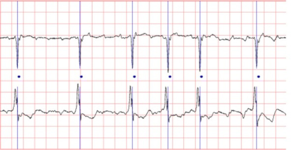
An atrial fibrillation (AF) is an irregular and rapid heart rate that can increase the risk of various heart-related complications, such as the stroke and the heart failure [1]. During an AF, the upper chambers of the heart beat work irregularly, and cannot coordinate with the lower chambers properly [2]. The symptoms of the AF often include the heart palpitation, the shortness of breath and the weakness [3]. The electrocardiogram (ECG) is an important tool to monitor and detect the AF. Figure 1 shows an example of AF waves of an ECG.
Fig. 1.
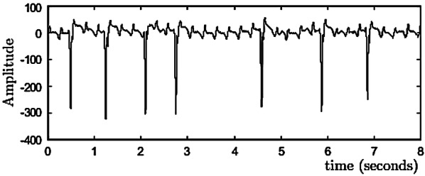
An example of AF waves [4]
An ECG having AFs has the following three main features: (1) the small and irregular F-wave with the baseline tremor replaces the normal P-wave; (2) the ventricular rate is extremely irregular; and (3) when ventricular rate becomes faster, aberrant ventricular conduction will happen and cause a wider QRS-wave [5].
There have been some researches for AF detection based on ECG [6–8]. However, most work concentrated on ECG detection rather than prediction [9, 1]. Detection is to find the AFs in the available ECG data, while prediction is modeling the probable trend of ECG. We find that if we can detect certain abnormalities before the happening of AFs, we can determine whether or not an AF will happen in the next phase.
From the medical point of view, the pathology of AF is difficult to predict. A number of researchers used deep learning techniques to detect AFs. In particular, the recurrent neural network (RNN), the long short term memory (LSTM) and the convolutional neural network (CNN) [10] are three popular deep learning models for AF detection. In general, CNNs have good performance on pattern recognition of graphics. However, some work [11] has shown that a CNN cannot perform as good as an RNN on the AF detection. The reason is that CNN cannot deal with the ‘time’ parameter and the potential gradient disappearance problem of time series as efficient as RNN.
An RNN is an efficient tool for time series modeling. It has the problem of gradient disappearance and gradient descent when backpropagation occurs. Hence, LSTM networks are proposed to solve this problem. However, a traditional LSTM only has one hidden layer, which limit the performance of the LSTM on feature extraction [12]. Therefore, we develop a stacked-LSTM architecture that has more hidden layers than the common LSTMs. Stacked hidden layers can significantly improve the performance of the feature extraction of ECGs. And the multiplicative structure is designed to allow transition functions to vary across inputs [13]. The performance of the AF prediction can then be improved. We call this architecture the Stacked LSTM for AF Prediction (SLAP). We conduct comprehensive experiments to evaluate the accuracy, recall and f-score of three models: RNN, LSTM and SLAP for AF prediction. Experiment results show that the SLAP performs much better than the RNN and the LSTM. In the experiment, the SLAP has 92% f-score, while the RNN and the LSTM only have 83% and 87% f-scores respectively.
Background
The RNN neural network
RNN is a popular tool to solve the time series problems.
Figure 2 shows an RNN structure. A time unit consists of an input layer , a hidden layer and an output layer . They are vectors whose sizes are set in advance. And the size determines the order of the weight matrix. The backward connections between the units connect the input series. The output of a unit influences the performance of the next unit. The relations of , , and are shown in Formulas (1) and (2) [14].
| 1 |
| 2 |
where U,W, and V represent the weights between the input layer and the hidden layer, the weights between two different time units, and the weights between the hidden layer and the output layer respectively. The order of a matrix is determined by the size of the vectors of the adjacent layers. and are the bias. The size of a bias is determined by the vector size of its calculated result. and are the longitudinal activation functions.
Fig. 2.
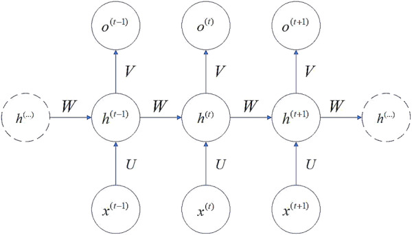
RNN Structure
The LSTM neural network
An LSTM layer is an advanced RNN. When RNN propagates backward, the defects of gradient disappearance and gradient explosion are easy to occur. To solve this problem, the LSTM selectively forgets or preserves information using a certain type of cells, namely forgetting cells. The LSTM integrates the memory and the current input, so that the previous memory will be retained rather than being affected by the multiplications. In an RNN, each memory unit multiplies a derivative of W and activation function, resulting in very large or very small gradient. However, in an LSTM, each cell calculates the elements that need to be forgotten in the current unit state. And each cell figures out the new memory state based on both the output of the upper unit and the input of the current unit. We use the gate structure to support this process (Fig. 4).
Fig. 4.

LSTM cell’s division of the gate structure
In Fig. 3, an LSTM cell includes three gates: the input gate, the forget gate and the output gate. The input gate dynamically pre-processes the continuously arriving ECG signals. The forget gate is used to select the information that need to be forgotten. The input and output gates are used to input data to the hidden layer and output the result to the next cell [15].
Fig. 3.
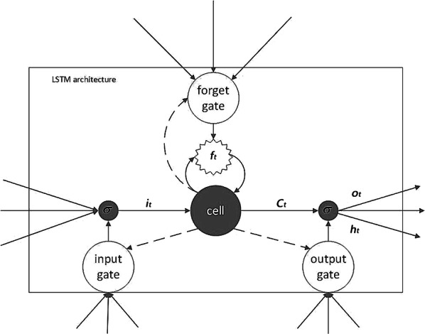
Structure of an LSTM cell
The input gate dynamically deals with the input data: a continuous time series. Formulas 3 and 4 show the weighted activation operation process, where represents the output of the input gate; and are respectively the weight matrix and the vector of bias in this gate; and are the input and output vectors of the upper cell respectively; and are respectively the weight matrix and bias for calculating ; tanh is its activation function; and is the intermediate variable for calculating the current memory .
| 3 |
| 4 |
The forget gate is used to select the information that needs to be retained in the current cell. Such information is represented by (see Formula 5). The non-retained information will be forgotten and will not influence the memory of the following cells.
| 5 |
In Formula 5, f is the output of the forget gate and is the retained information of the upper cell. is the calculated result of Formula 4. Formula 6 shows the calculation of .
| 6 |
where and are the weight matrix and the bias vector in this gate respectively.
The output gate outputs the weighted result , which is calculated based on the previous output , the current intput , and the current memory (see Formulas 7 and 8).
| 7 |
| 8 |
where and are the weight matrix and the bias vector in this gate respectively.
Figure 4a–d respectively show the working procedures of the forget gate (Formula 6), the input gate (Formulas 3 and 4), the s calculation (Formula 5), and the output gate (Formulas 7 and 8).
A stacked-LSTM architecture for AF prediction
We design SLAP and use the Gaussian distribution to model the multivariate ECG signals.
A stacked-LSTM architecture
The structure of SLAP is shown in Fig. 5. It has two LSTM sub-layers, which are connected together by using different types of weight parameters. The detailed structure of SLAP layers is shown in Fig. 6.
Fig. 5.

Stacked-LSTM for AF prediction
Fig. 6.
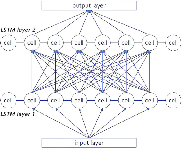
The detailed structure of SLAP
In Fig. 6, a stacked-LSTM repeatedly overlays the LSTM hidden layer on a single-layer LSTM structure. And the output of the upper hidden layer is the input of the next hidden layer. A cell corresponds to a time unit. Each edge has a weight value. The input of a cell is a multivariate time series and the output is a time series having N cells. Formula 9 defines the data transformation process.
| 9 |
In Formula 9, is the input data of a next hidden layer in SLAP; is the weight of the edge that connects the previous output and the next layer’s input; Num is the size of the previous layer’s output; is the output value for one cell; is the bias; and f is the activation function. This structure is similar to the hidden layer structure in artificial neural networks [16].
The design of stacked structure improves the performance of the feature extraction. It allows different weight matrixes and biases for ECG data. The LSTM cells are good at controlling the flow of information. SLAP has the advantages of both the multiplicative structure and the LSTM cells.
Based on the new input sequence, the output of the last time unit of an SLAP is used for subsequent prediction to predict and detect AFs. Overall, the trained SLAP model can be used to predict the future ECG signals during variable time lengths. Then we can classify the abnormal AF heartbeat based on the predicted values.
The fitting of multivariate gaussian distribution
We use the multivariate gaussian distribution to fit the errors between the predicted values and the true values. For training sets (all normal samples), errors between multiple predictions and standard values are calculated without extracting their professional medical features. If the next time period includes a normal sample, the difference between the predicted sample and the true sample will be very small. Here we use a threshold to measure the difference of the error between normal and abnormal samples and standard samples.
If the error is subjected to a certain probability distribution P, we can see it as an exception with p(x), where is a very small constant. We assume that P is a Gaussian distribution. Even if the actual error does not conform to a Gaussian distribution, our assumption can also lead to a good classification result through adjusting some parameters [17].
We use the Gaussian distribution to fit () based on the maximum likelihood estimation (MLE). However, because the points in the time series are not independent to each other, we adopt the multivariate Gaussian distribution to fit the multivariate ECGs. In addition, we need to learn the mean vector (Formula 10) and the covariance matrix (Formula 11).
| 10 |
| 11 |
where m is the size of each sample; represents the j-th element in the i-th sample; is an n × 1 vector; and is an n × n matrix.
The multivariate Gaussian distribution is calculated by Formula 12:
| 12 |
Network learning
We introduce the steps of learning the stacked LSTM.
Step 1: Data preparation
The ECG dataset for learning an SLAP model is a multi-variate time series X (x1,…,xn), where in X is a time-dependent variable. We first divide this dataset into four subsets: A, B, C and D.
Set A includes 40 normal samples of 256 time units in about 2 s. It is used to train the stacked-LSTM network. Set B has similar number of normal samples with Set A. Set B is used to stop the training model after reaching a certain precision standard. Set C includes 32 normal samples and 8 AF termination samples. It is used to find the exception threshold. Set D includes 20 normal samples and 20 AF termination samples. It is used for model testing.
Step 2: The determination of the threshold
After fitting the multivariate Gaussian distribution, we need to determine the value of the threshold . It is used to judge whether the sample is abnormal or not. For sample x, if p(x), it will be classified as an abnormal sample.
For each sequence X (, ,… ) in set B, do (n-l) times of prediction, l is the position of the first element in the error subsequence of input sequence whose element is computed n times. n is the length of the sequence. l is the length of the input. After doing that, each element in the subsequence [l,n-l] is predicted (n-l) times. Then an error vector = [, ,… ] is constructed to calculate the error of each element compared with the true value. The j-th () element in that vector represents the error of the j-th prediction. at last, we calculate all the time points matching the conditions and construct an error matrix of size (n − l) × (n − l).
We use the matrix constructed above to fit the multivariate Gaussian distribution. Each row of the matrix is the variable of Gaussian distribution. Sets A and B generate the error matrix. They are also used for training and fitting the multivariate Gaussian distribution. Next, we use set C to approximate the exception threshold . We then get more precise values of by maximizing f-score. The f-score is calculated by Formula 13 [12]:
| 13 |
where represents the accuracy rate. It is defined by Formula 14. represents the recall rate of the results. It is the output rate of the true results and is defined by Formula 15 [9]. is the indicator that controls the accuracy rate and the recall rate. That is, the smaller of , the more contributions the accuracy rate will have to the f-score.
| 14 |
| 15 |
Experiments
Datasets
Our experiments are based on the Long-term AF database and the AF terminal challenge database1. The long-term AF database includes 84 long-term ECG recordings of subjects with paroxysmal or sustained AF [18]. Each record contains two simultaneously recorded ECG signals that are digitized at 128 Hz with 12-bit resolution over a 20 mV range. The record duration is in 24 to 25 h. Figure 7 shows a subset of a record.
Fig. 7.
A data stream of long-term AF database
Parameter setting and experiment results
Table 1 shows the parameter definitions for training an SLAP. The length of time series received by input layer is 100. The output length of the predicted time series is 10. That is to say, a long-time ECG is divided into several segments, where each segment is 100 unit time, and each unit time is about 1 second. The input length of each segment is within 1–2 min. There are two hidden LSTM layers in the SLAP, and 55 cells in each layer. The learning rate of the model is 10e−3, the error of termination training is 10e−6, and the β for calculating F score is set to 0.1.
Table 1.
Parameter presupposition
| Parameters | Values | Parameters | Values |
|---|---|---|---|
| Input size | 100 | Training times | 500 |
| Cells number | 110 | Stopping value | 10e−6 |
| Layers | 2 | Learning rate | 10e−3 |
| Output size | 10 | β | 0.1 |
After about 1 h training, the Stacked-LSTM Neural Network has a preliminary predictive ability. Figure 8 shows the real values and the predicted values. The blue line is the true value and the red dotted line is the predicted value.
Fig. 8.
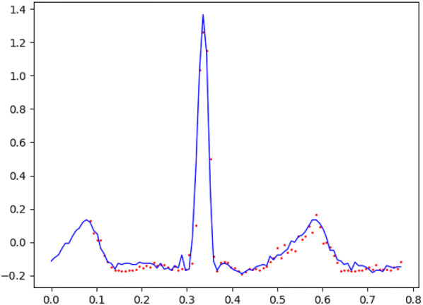
Comparison between the predictive values and the true values
The final threshold ε and the f-score are 0.015 and 0.92 respectively. We use this threshold to test the anomaly prediction based on set D. We set the accuracy rate as 0.92 and the recall rate as 0.9. Time for searching the threshold is maintained at about 45 seconds. Each time series for testing spends less than 0.1 s to find the AFs. The experiment is run on a computer with a GPU of NVIDIA GeForce 1050.2
The final result divides the time series into n segments, and evaluates the symptoms of each segment separately. Through observation, we find that the abnormal segments mostly show the disappearance of the normal P wave and the increase of the F wave frequency.
We compare the AF prediction performance of the SLAP and the performance of the single-layer LSTM and RNN. Table 1 shows the settings of the learning rates, the stopping values, the sizes of inputs and outputs, and the searching thresholds of the single-layer LSTM and the RNN. Table 2 shows the prediction results.
Table 2.
Comparison of the results of different models
| Model | RNN | LSTM | SLAP |
|---|---|---|---|
| Accuracy | 0.83 | 0.87 | 0.92 |
| Recall | 0.87 | 0.88 | 0.92 |
| F-score | 0.83 | 0.87 | 0.92 |
In Table 2, the final f-score of single-layer LSTM is 0.87, which is better than 0.83 of traditional RNN. The f-score of the SLAP is higher than that of the single-layer LSTM. We can see that the SLAP which has multiple layers has the highest performance in the AF detection from ECGs.
We also compare the SLAP with different layer numbers. Table 3 shows the comparison results.
Table 3.
Comparison of the results with different layer numbers
| Layer number | 1 | 2 | 3 |
|---|---|---|---|
| Accuracy | 0.87 | 0.92 | 0.84 |
| Recall | 0.88 | 0.92 | 0.7 |
| F-score | 0.87 | 0.92 | 0.84 |
In Table 3, when the number of layers is 2, the maximum value is obtained. It is because when the number of layers is small, the model lacks diversity. When the number of layers is large, the phenomenon of under-fitting occurs. An efficient way to avoid under-fitting is to increase data size and iteration times.
The result comparison shows that LSTM has a better performance in dealing with long-term ECGs. SLAP has the optimal performance among the three prediction models, because the stacked LSTM layers can extract high-level features [10]. This type of features makes the model’s f-score higher and results in a richer output [12]. The test results show that p(t) of the abnormal data is usually small, so it is suitable to fit multivariate Gaussian distribution to solve the problem.
Conclusion
In this paper, we develop an AF prediction model which uses a special kind of RNN network called SLAP. With the help of this model, we can analyze patients’ ECG signals and forecast the AF in advance. We also conduct comprehensive experiments based on two public datasets. The experiment result is promising and better than the state-of-the-art AF detection architectures like the RNN and the LSTM.
Funding
This work is supported by the National Natural Science Foundation of China (Grant No. 61702274) and the Natural Science Foundation of Jiangsu Province (Grant No. BK20170958), and PAPD.
Footnotes
Long-term AF database and AF terminal challenge database is available on:https://physionet.org/.
Tenorflow’s programs can be accelerated using NVIDIA GPU drivers, the driver is available on: https://developer.nvidia.com/cudnn.
Publisher's Note
Springer Nature remains neutral with regard to jurisdictional claims in published maps and institutional affiliations.
References
- 1.Yuan C, Yan Y, Zhou L, Bai J, Wang L. Automated atrial fibrillation detection based on deep learning network. In: 2016 IEEE international conference on information and automation. 2016. pp. 1159–64.
- 2.Arruda M, Natale A. Ablation of permanent AF. J Interv Cardiac Electrophysiol. 2008;23(1):51–57. doi: 10.1007/s10840-008-9252-z. [DOI] [PubMed] [Google Scholar]
- 3.Callahan T, Baranowski B. Managing newly diagnosed atrial fibrillation: rate, rhythm, and risk. Cleve Clin J Med. 2011;78(4):258–64. doi: 10.3949/ccjm.78a.09165. [DOI] [PubMed] [Google Scholar]
- 4.Rieta JJ, Zarzoso V, Millet-Roig J, García-Civera R, Ruiz-Granell R. Atrial activity extraction based on blind source separation as an alternative to QRST cancellation for atrial fibrillation analysis. Comput Cardiol. 2000;2000:69–72. [Google Scholar]
- 5.Lu Xilie, Tan Xuerui, and Xu Yong. ECG analysis of atrial fibrillation. People’s Publishing House 2011.
- 6.Sinha AM, Diener HC, Morillo CA, Sanna T, Bernstein RA, Di Lazzaro V, Brachmann J. Cryptogenic stroke and underlying atrial fibrillation (CRYSTAL AF): design and rationale. Am Heart J. 2010;160(1):36–41. doi: 10.1016/j.ahj.2010.03.032. [DOI] [PubMed] [Google Scholar]
- 7.Häußinger K, Stanzel F, Huber RM, Pichler J, Stepp H. Autofluorescence detection of bronchial tumors with the D-Light/AF. Diagn Ther Endosc. 1999;5(2):105–112. doi: 10.1155/DTE.5.105. [DOI] [PMC free article] [PubMed] [Google Scholar]
- 8.Thijs VN, Brachmann J, Morillo CA, Passman RS, Sanna T, Bernstein RA, Rogers TB. Predictors for atrial fibrillation detection after cryptogenic stroke: results from CRYSTAL AF. Neurology. 2016;86(3):261–269. doi: 10.1212/WNL.0000000000002282. [DOI] [PMC free article] [PubMed] [Google Scholar]
- 9.Chauhan S, Vig L. Anomaly detection in ECG time signals via deep long short-term memory networks. In: 2015 IEEE international conference on data science and advanced analytics. 2015. pp. 1–7.
- 10.Xiong Z, Stiles MK, Zhao J. Robust ECG signal classification for detection of atrial fibrillation using a novel neural network. In: 2017 computing in cardiology. 2017. pp. 1–4.
- 11.Shashikumar SP, Shah AJ, Li Q, Clifford GD, Nemati S. A deep learning approach to monitoring and detecting atrial fibrillation using wearable technology. In: 2017 IEEE EMBS international conference on biomedical & health informatics. 2017. pp. 141–44.
- 12.Malhotra P, Vig L, Shroff G, Agarwal P. Long short term memory networks for anomaly detection in time series, Vol. 89. Presses universitaires de Louvain. 2015.
- 13.Krause B, Lu L, Murray I, Renals S. Multiplicative LSTM for sequence modelling. ArXiv preprint arXiv:1609.07959 (2016).
- 14.Hochreiter S, Schmidhuber J. Long short-term memory. Neural Comput. 1997;9(8):1735–1780. doi: 10.1162/neco.1997.9.8.1735. [DOI] [PubMed] [Google Scholar]
- 15.Cheng M, Xu Q, Lv J, Liu W, Li Q, Wang J. MS-LSTM A multi-scale LSTM model for BGP anomaly detection. In: 2016 IEEE 24th international conference on network protocols. 2016. pp. 1–6.
- 16.Rai HM, Trivedi A, Shukla S. ECG signal processing for abnormalities detection using multi-resolution wavelet transform and Artificial Neural Network classifier. Measurement. 2013;46(9):3238–3246. doi: 10.1016/j.measurement.2013.05.021. [DOI] [Google Scholar]
- 17.Hundman K, Constantinou V, Laporte C, Colwell I, Soderstrom T. Detecting spacecraft anomalies using lstms and nonparametric dynamic thresholding. In: 24th ACM SIGKDD international conference on knowledge discovery & data mining. 2015. pp. 387–95.
- 18.Li H, Wang Y, Wang H, Zhou B. Multi-window based ensemble learning for classification of imbalanced streaming data. World Wide Web. 2017;20(6):1507–1525. doi: 10.1007/s11280-017-0449-x. [DOI] [Google Scholar]