Modelling the COVID-19 epidemic and implementation of population-wide interventions in Italy

Abstract

In Italy, 128,948 confirmed cases and 15,887 deaths of people who tested positive for SARS-CoV-2 were registered as of 5 April 2020. Ending the global SARS-CoV-2 pandemic requires implementation of multiple population-wide strategies, including social distancing, testing and contact tracing. We propose a new model that predicts the course of the epidemic to help plan an effective control strategy. The model considers eight stages of infection: susceptible (S), infected (I), diagnosed (D), ailing (A), recognized (R), threatened (T), healed (H) and extinct (E), collectively termed SIDARTHE. Our SIDARTHE model discriminates between infected individuals depending on whether they have been diagnosed and on the severity of their symptoms. The distinction between diagnosed and non-diagnosed individuals is important because the former are typically isolated and hence less likely to spread the infection. This delineation also helps to explain misperceptions of the case fatality rate and of the epidemic spread. We compare simulation results with real data on the COVID-19 epidemic in Italy, and we model possible scenarios of implementation of countermeasures. Our results demonstrate that restrictive social-distancing measures will need to be combined with widespread testing and contact tracing to end the ongoing COVID-19 pandemic.

A new epidemiological model, termed SIDARTHE, distinguishes between diagnosed and undiagnosed cases of SARS-CoV-2 infection, as well as modeling effects of social distancing and widespread testing, to predict possible outcomes of the COVID-19 epidemic in Italy.

Main

After a novel strain of coronavirus, SARS-CoV-2, was identified in Wuhan (Hubei), China^1,2, an exponentially growing number of patients in mainland China were diagnosed with COVID-19, prompting Chinese authorities to introduce radical measures to contain the outbreak³. Despite these measures, a COVID-19 pandemic ensued in the following months. The World Health Organisation report dated 5 April 2020 reported 1,133,758 total cases and 62,784 deaths worldwide⁴.

Italy has been severely affected⁵. After the first indigenous case on 21 February 2020 in Lodi province, several suspect cases (initially epidemiologically linked) began to emerge in the south and southwest territory of Lombardy⁶. A ‘red zone’, encompassing 11 municipalities where SARS-CoV-2 infection was endemic, was instituted on 22 February 2020, and put on lockdown to contain the emerging threat. A campaign to identify and screen all close contacts with confirmed cases of COVID-19 resulted in taking 691,461 nasal swabs as of 5 April 2020. Of the 128,948 detected cases, 91,246 were currently infected (28,949 hospitalized, 3,977 admitted to intensive care units (ICUs) and 58,320 quarantined at home), 21,815 had been discharged due to recovery and 15,887 had died⁷. In the early days of the epidemic in Italy, both symptomatic and asymptomatic people underwent screening. A government regulation dated 26 February 2020 limited screening to symptomatic subjects only⁸. On 8 March 2020, to further contain the spread of SARS-CoV-2, the red zone was extended to the entire area of Lombardy and 14 more northern Italian provinces. On 9 March 2020, lockdown was declared for the entire country⁹ and progressively stricter restrictions were adopted.

COVID-19 displays peculiar epidemiological traits when compared with previous coronavirus outbreaks of SARS-CoV and MERS-CoV. According to Chinese data¹⁰, a large number of transmissions, both in nosocomial and community settings, occurred through human-to-human contact with individuals showing no or mild symptoms. The estimated basic reproduction number (R₀) for SARS-CoV-2 ranges from 2.0 to 3.5^11–13, which seems comparable, or possibly higher, than for SARS-CoV and MERS-CoV. High viral loads of SARS-CoV-2 were found in upper respiratory specimens of patients showing little or no symptoms, with a viral shedding pattern akin to that of influenza viruses¹⁴. Hence, inapparent transmission may play a major and underestimated role in sustaining the outbreak.

Predictive mathematical models for epidemics^15–18 are fundamental to understand the course of the epidemic and to plan effective control strategies. One commonly used model is the SIR model¹⁹ for human-to-human transmission, which describes the flow of individuals through three mutually exclusive stages of infection: susceptible, infected and recovered. More complex models can accurately portray the dynamic spread of specific epidemics. For the COVID-19 pandemic, several models have been developed. Lin and colleagues extended a SEIR (susceptible, exposed, infectious, removed) model considering risk perception and the cumulative number of cases²⁰, Anastassopoulou and colleagues proposed a discrete-time SIR model including dead individuals²¹, Casella developed a control-oriented SIR model that stresses the effects of delays and compares the outcomes of different containment policies²² and Wu and colleagues used transmission dynamics to estimate the clinical severity of COVID-19²³. Stochastic transmission models have also been considered^24,25. Here, we propose a new mean-field epidemiological model for the COVID-19 epidemic in Italy that extends the classical SIR model, similar to that developed by Gumel and colleagues for SARS²⁶. A summary of the main findings, limitations and implications of the model for policymakers is shown in Table 1.

Table 1.

Policy summary

Background	Curbing the global spread of SARS-CoV-2 requires implementation of multiple population-wide strategies; however, how the timing and stringency of such measures will affect ‘flattening the curve’ remains unknown. We have proposed a new model that predicts the evolution of epidemics and helps to assess the impact of different strategies to contain the spread of the infection, including lockdown and social distancing, as well as testing and contact tracing.
Main findings and limitations	Testing is important because undetected infected people, most of whom are asymptomatic, largely sustain the epidemic spread. Several possible scenarios have been outlined. Under the less stringent lockdown conditions with limited testing, we predict that more than 70,000 people could die in Italy in the first year. However, if strict lockdown measures continue to be maintained and population-wide testing and contact tracing efforts are substantially increased, the number of deaths could potentially be limited to 25,000 people overall. As with all modeling studies, our predictions are based on reasonable assumptions, but the actual course of the epidemic heavily relies on how and when isolation and safety measures are implemented.
Policy implications	Our findings confirm that the adopted social-distancing measures are necessary and effective, and should be promptly enforced at the earliest stage. Lockdown measures can only be relieved safely in the presence of widespread testing and contact tracing. Combining lockdown and population-wide testing is key to rapidly ending the COVID-19 pandemic.

Our model, named SIDARTHE, discriminates between detected and undetected cases of infection and between different severity of illness (SOI), non-life-threatening cases (asymptomatic and pauci-symptomatic; minor and moderate infection) and potentially life-threatening cases (major and extreme) that require ICU admission.

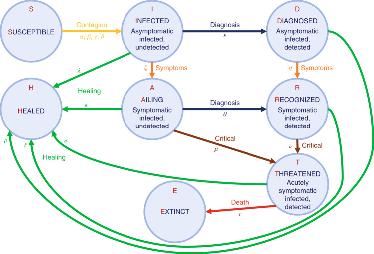
The total population is partitioned into eight stages of disease: S, susceptible (uninfected); I, infected (asymptomatic or pauci-symptomatic infected, undetected); D, diagnosed (asymptomatic infected, detected); A, ailing (symptomatic infected, undetected); R, recognized (symptomatic infected, detected); T, threatened (infected with life-threatening symptoms, detected); H, healed (recovered); E, extinct (dead). The interactions among these stages are shown in Fig. 1. We omit the probability rate of becoming susceptible again after having recovered from the infection. Although anecdotal cases are found in the literature²⁷, the reinfection rate value appears negligible. A detailed discussion of the model considerations and parameters is provided in the Methods.

Fig. 1. The model.

Graphical scheme representing the interactions among different stages of infection in the mathematical model SIDARTHE: S, susceptible (uninfected); I, infected (asymptomatic or pauci-symptomatic infected, undetected); D, diagnosed (asymptomatic infected, detected); A, ailing (symptomatic infected, undetected); R, recognized (symptomatic infected, detected); T, threatened (infected with life-threatening symptoms, detected); H, healed (recovered); E, extinct (dead).

For the COVID-19 epidemic in Italy, we estimate the model parameters based on data from 20 February 2020 (day 1) to 5 April 2020 (day 46) and show how the progressive restrictions, including the most recent lockdown progressively enforced since 9 March 2020, have affected the spread of the epidemic. We also model possible longer-term scenarios illustrating the effects of different countermeasures, including social distancing and population-wide testing, to contain SARS-CoV-2.

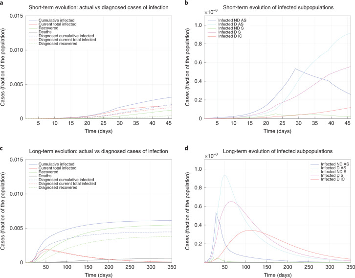
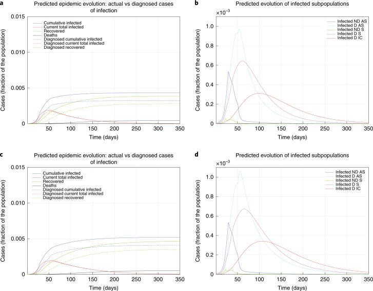
The model parameters have been updated over time to reflect the progressive introduction of increased restrictions. On day 1, the basic reproduction number was R₀ = 2.38, which resulted in a substantial outbreak. On day 4, R₀ = 1.66 as a result of the introduction of basic social distancing, awareness of the epidemic, hygiene and behavioral recommendations, and early measures by the Italian government (for example, closing schools). At day 12, asymptomatic individuals were almost no longer detected, and screening was focused on symptomatic individuals (leading to R₀ = 1.80). On day 22, a partially incomplete lockdown, of which the effectiveness was reduced by the movement of people from the north to the south of Italy when the country-wide lockdown was announced but not yet enforced, yielded R₀ = 1.60. When the national lockdown was fully operational and strictly enforced, after day 28, R₀ = 0.99, finally reaching below 1. Moreover, R₀ = 0.85 was achieved after day 38 due to a wider testing campaign that identified more mildly symptomatic infected individuals. Figure 2a shows the model evolution with the estimated parameters up to day 46; in the earliest epidemic phase, the number of infected was considerably underestimated. Of the total cases, 35% were undetected. In Fig. 2b, the infected individuals are partitioned into the different subpopulations (diagnosed or not, with different SOI classification). Over a 350-day horizon, in the absence of further policy changes, Fig. 2c predicts that 0.61% of the population will contract the virus (and 0.45% will be diagnosed), while 0.06% of the population will die from COVID-19. The peak of the number of concurrently infected individuals will occur on around day 50 at 0.19% of the population, while the peak of concurrently diagnosed infected individuals will occur later (around day 56) and amounts to 0.17% of the population. The actual case fatality rate (CFR) is 9.8% and the perceived CFR is 13%. Figure 2d shows that each infected subpopulation reaches its peak at a different time.

Fig. 2. Fitted and predicted epidemic evolution.

Epidemic evolution predicted by the model based on the available data about the COVID-19 outbreak in Italy. a,b, The short-term epidemic evolution obtained by reproducing the data trend with the model. c,d, The long-term predicted evolution over a 350-day horizon. a,c, The difference between the actual evolution of the epidemic (solid lines; this refers to all cases of infection, both diagnosed and non-diagnosed, predicted by the model, although non-diagnosed cases are of course not counted in the data) and the diagnosed epidemic evolution (dashed lines; this refers to all cases that have been diagnosed and are thus reported in the data). The plots in b and d distinguish between the different categories of infected patients: non-diagnosed asymptomatic (ND AS), diagnosed asymptomatic (D AS), non-diagnosed symptomatic (ND S), diagnosed symptomatic (D S) and diagnosed with life-threatening symptoms (D IC). Note that a,c and b,d have different scales.

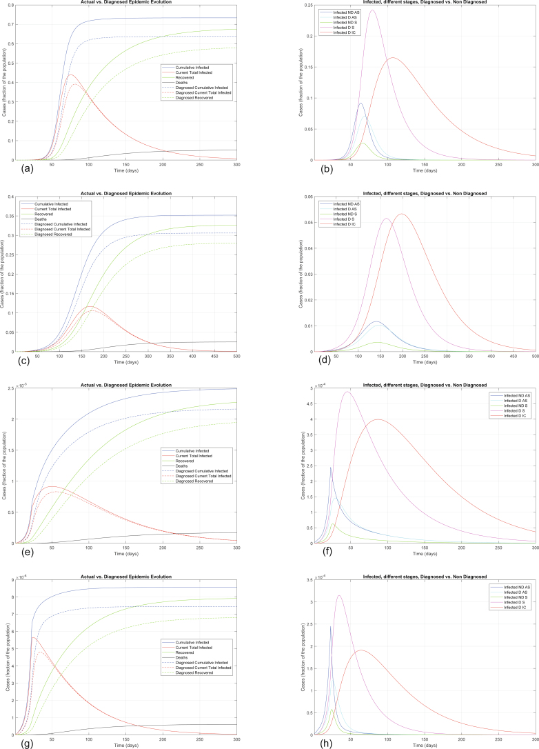
Extended Data Fig. 1 shows how the situation could have evolved if milder or stronger measures had been implemented earlier. The curve following day 22 shows the importance and effectiveness of a prompt lockdown. The actual epidemic evolution corresponds to an intermediate scenario: the lockdown measures had a moderate effect, probably due to their incremental nature.

Extended Data Fig. 1. Alternative scenarios for epidemic evolution.

Epidemic evolution that would have been predicted by the model for the COVID-19 outbreak in Italy if, after day 22, social-distancing countermeasures had been: absent (panels a and b), mild (panels c and d), strong (panels e and f) and very strong (panels g and h). In all cases, the actual Case Fatality Rate is around 7.2%, while the perceived CFR is around 9.0%. Panels (a), (c), (e), (g) show the difference between the actual (real cases) and the perceived (diagnosed cases) evolution of the epidemics, while panels (b), (d), (f), (h) distinguish between the different categories of infected patients. Note the different scales between the panels, having different orders of magnitude, which testify the enormous impact of social-distancing and lockdown.

We predict a range of possible future scenarios, with different measures enforced after day 50.

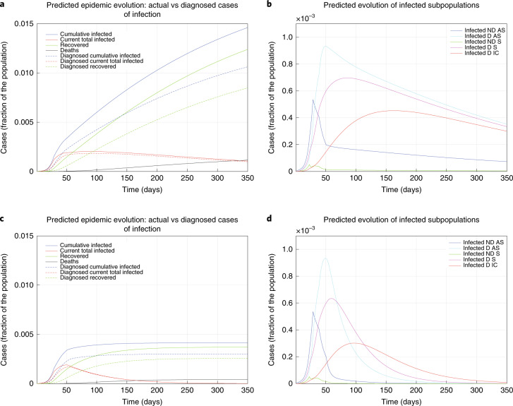
Figure 3a,b shows, if the lockdown is weakened, a sudden and strong increase of the spread of disease, a prolonged emergency and more deaths (0.12% of the population in the first 350 days). Figure 3c,d shows the benefits of stricter lockdown measures: after 350 days, 0.41% of the population would contract the virus (0.30% diagnosed) and 0.04% of the population would die.

Fig. 3. The effect of lockdown.

a–d, Epidemic evolution predicted by the model for the COVID-19 outbreak in Italy when, after day 50, the social distancing countermeasures are weakened, leading to a larger R₀ = 0.98 (a,b), or strengthened, leading to a smaller R₀ = 0.50 (c,d). a,c, The difference between the actual (real cases) and perceived (diagnosed cases) evolution of the epidemics. The plots in b and d distinguish between the different categories of infected patients: non-diagnosed asymptomatic (ND AS), diagnosed asymptomatic (D AS), non-diagnosed symptomatic (ND S), diagnosed symptomatic (D S) and diagnosed with life-threatening symptoms (D IC). Note that a,c and b,d have different scales.

A policy of population-wide testing and contact tracing would help to rapidly end the epidemic, as suggested by Peto²⁸. Figure 4a,b shows the effect of such measures: the peak would be reached sooner and, after 350 days, 0.43% of the population would contract the virus (0.33% diagnosed), with an estimated 0.05% dying. Figure 4c,d shows the effect of combining a milder lockdown with widespread testing and contact tracing: after 350 days, 0.52% of the population would contract the virus (0.41% diagnosed) and 0.05% would die.

Fig. 4. The effect of testing.

a–d, Epidemic evolution predicted by the model for the COVID-19 outbreak in Italy when, after day 50, massive testing and contact tracing is enforced (a,b), leading to R₀ = 0.59, as well as in parallel with weakening social-distancing measures (c,d), leading to R₀ = 0.77. The plots in a and c show the difference between the actual (real cases) and the perceived (diagnosed cases) evolution of the epidemics. The plots in b and d distinguish between the different categories of infected patients: non-diagnosed asymptomatic (ND AS), diagnosed asymptomatic (D AS), non-diagnosed symptomatic (ND S), diagnosed symptomatic (D S) and diagnosed with life-threatening symptoms (D IC). Note that a,c and b,d have different scales.

Hence, the current adopted lockdown measures are vital to contain the epidemic and cannot be relieved. Rather, they should be even more restrictive. The enforced lockdown could be mitigated in the presence of widespread testing and contact tracing, which would strongly contribute to a rapid resolution of the epidemic.

Distinguishing between diagnosed and non-diagnosed cases highlights a distortion in disease statistics. The discrepancy between the actual CFR (total number of deaths due to the infection, divided by the total number of infected people) and the perceived CFR (number of deaths ascribed to the infection, divided by the number of people diagnosed as infected) can be quantified, which explains the gap between the actual infection dynamics and perception of the outbreak. Performing an insufficient number of tests underestimates the transmission rate and overestimates the CFR. Our model can predict the long-term effects of underdiagnosis.

Concerning diagnostic tests for COVID-19, currently, standard molecular methods to detect the presence of SARS-CoV-2 in respiratory samples are based on non-specific real-time polymerase chain reaction with reverse transcription methods, which target RNA-dependent RNA polymerase and E genes²⁹. These tests are time-consuming and cannot be done on all susceptible individuals in the population; high false negatives rates have been reported and certified laboratories with expensive equipment are needed. Rapid tests with high sensitivity and specificity that can be easily adapted to real-life settings (schools, airports, train stations) are urgently required. Some laboratories are moving in this direction, developing a 15 min test to detect SARS-CoV-2 immunoglobulins IgM and IgG simultaneously in human blood³⁰.

Our model confirms that diagnosis campaigns can reduce the infection peak (the diagnosed population enters quarantine and is therefore less likely to affect the susceptible population) and help end the epidemic more quickly²⁸. Healthcare workers are more likely to be exposed and their risk of infection is increased, as supported by reports from China^31,32 suggesting that disease amplification in healthcare settings will occur despite restrictive measures.

The model does not consider reduced availability of medical care due to the healthcare system reaching or even surpassing its capacity³³. These analyses can only be done indirectly. For example, when the number of seriously affected individuals is high (above a threshold), the mortality coefficient will be increased due to an insufficient number of ICUs.

We compare scenarios with control measures of varying strength and nature, predicting for each the timing and magnitude of the epidemic peak, including the peak of ICU admissions. According to our findings, a partial implementation of lockdown measures results in a delay in the peak of infected individuals and patients admitted to the ICU, contrasting with an only moderate decrease in the total number of infected individuals and ICU admissions. Conversely, the implementation of very strong social-distancing strategies would result in an anticipated lower peak of infected individuals and patients admitted to the ICU, with a marked decrease in the total number of infected individuals and ICU admissions due to the disease.

Our findings provide policymakers with a tool to assess the consequences of possible strategies, including lockdown and social distancing, as well as testing and contact tracing. Our simulation results, achieved by combining the model with the available data about the COVID-19 epidemic in Italy, suggest that enforcing strong social-distancing measures is urgent, necessary and effective, in line with other reports in the literature^2,22,24. The earlier the lockdown is enforced, the stronger the effect obtained. The model results also confirm the benefits of mass testing, whenever facilities are available²⁸. We believe these indications can be useful to manage the epidemic in Italy, as well as in countries that are still in the early stages of outbreak.

Although the mortality rate (number of deaths in the whole population) of COVID-19 can be decreased with restrictive measures that reduce the spread of SARS-CoV-2, the CFR (number of deaths in the infected population) is essentially constant in different scenarios, unaffected by the extent of social restriction and testing. Despite rigid isolation policies, COVID-19 patients may still be burdened with excess case fatality, and efforts should be focused on developing more effective treatment strategies to combat COVID-19. As new drugs and vaccines are being tested and evaluated, the current scenario will evolve to account for these ongoing innovations^34–37.

Methods

SIDARTHE mathematical model

The SIDARTHE dynamical system consists of eight ordinary differential equations, describing the evolution of the population in each stage over time:

$$\dot{S}\left(t\right)=-S\left(t\right)\left(\alpha I\left(t\right)+\beta D\left(t\right)+\gamma A\left(t\right)+\delta R\left(t\right)\right)$$ 1

$$\dot{I}\left(t\right)=S\left(t\right)\left(\alpha I\left(t\right)+\beta D\left(t\right)+\gamma A\left(t\right)+\delta R\left(t\right)\right)-\left(\epsilon +\zeta +\lambda \right)I\left(t\right)$$ 2

$$\dot{D}\left(t\right)=\epsilon I\left(t\right)-\left(\eta +\rho \right)D\left(t\right)$$ 3

$$\dot{A}\left(t\right)=\zeta I\left(t\right)-\left(\theta +\mathrm{\mu }+\kappa \right)A\left(t\right)$$ 4

$$\dot{R}\left(t\right)=\eta D\left(t\right)+\theta A\left(t\right)-\left(\nu +\xi \right)R\left(t\right)$$ 5

$$\dot{T}\left(t\right)=\mathrm{\mu }A\left(t\right)+\nu R\left(t\right)-\left(\sigma +\tau \right)T\left(t\right)$$ 6

$$\dot{H}\left(t\right)=\lambda I\left(t\right)+\rho D\left(t\right)+\kappa A\left(t\right)+\xi R\left(t\right)+\sigma T\left(t\right)$$ 7

$$\dot{E}\left(t\right)=\tau T\left(t\right)$$ 8

where the uppercase Latin letters (state variables) represent the fraction of population in each stage, and all the considered parameters, denoted by Greek letters, are positive numbers. The interactions among different stages of infection are visually represented in the graphical scheme in Fig. 1. The parameters are defined as follows:

• α, β, γ and δ respectively denote the transmission rate (the probability of disease transmission in a single contact multiplied by the average number of contacts per person) due to contacts between a susceptible subject and an infected, a diagnosed, an ailing or a recognized subject. Typically, α is larger than γ (assuming that people tend to avoid contacts with subjects showing symptoms, even though diagnosis has not been made yet), which in turn is larger than β and δ (assuming that subjects who have been diagnosed are properly isolated). These parameters can be modified by social-distancing policies (for example, closing schools, remote working, lockdown). The risk of contagion due to threatened subjects, treated in proper ICUs, is assumed negligible.

• ε and θ capture the probability rate of detection, relative to asymptomatic and symptomatic cases, respectively. These parameters, also modifiable, reflect the level of attention on the disease and the number of tests performed over the population: they can be increased by enforcing a massive contact tracing and testing campaign²⁸. Note that θ is typically larger than ε, as a symptomatic individual is more likely to be tested.

• ζ and η denote the probability rate at which an infected subject, respectively not aware and aware of being infected, develops clinically relevant symptoms, and are comparable in the absence of specific treatment. These parameters are disease-dependent, but may be partially reduced by improved therapies and acquisition of immunity against the virus.

• µ and ν respectively denote the rate at which undetected and detected infected subjects develop life-threatening symptoms; they are comparable if there is no known specific treatment that is effective against the disease, otherwise µ may be larger. Conversely, ν may be larger because infected individuals with more acute symptoms, who have a higher risk of worsening, are more likely to have been diagnosed. These parameters can be reduced by means of improved therapies and acquisition of immunity against the virus.

• τ denotes the mortality rate (for infected subjects with life-threatening symptoms) and can be reduced by means of improved therapies.

• λ, κ, ξ, ρ and σ denote the rate of recovery for the five classes of infected subjects; they may differ significantly if an appropriate treatment for the disease is known and adopted for diagnosed patients, but are probably comparable otherwise. These parameters can be increased thanks to improved treatments and acquisition of immunity against the virus.

Discussion on modeling choices

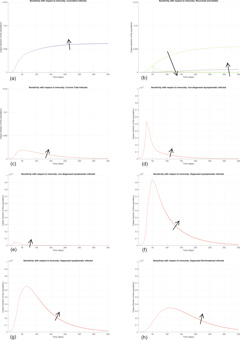
In the model, we omit the probability rate of becoming susceptible again, after having already recovered from the infection, because this appears to be negligible based on early evidence²⁷. Given the scarcity of available data, it is impossible to have conclusive evidence about immunity at this stage. Immunity might also be temporary³⁸. Although some reports suggest the possibility of SARS-CoV-2 reinfection^27,39,40, the indicated presence of viral RNA in respiratory samples might reflect a persistence rather than a true recurrence. The literature on the recrudescence of related members of the coronavirus family, such as SARS-CoV and MERS-CoV, is similarly sporadic. MERS-CoV reinfection despite serum detection of neutralizing antibodies has been described only in animals^41,42, while the presence of neutralizing antibodies in serum via primary infection or passive transfer has been shown to prevent respiratory tract replication of SARS-CoV in a murine model⁴³. From a modeling perspective, we are particularly interested in predictions over a relatively short horizon within which the temporary immunity is likely still to be in place, and the possibility of reinfection would negligibly affect the total number of susceptible individuals and so there would be no substantial difference in the evolution of the epidemic curves we consider. To provide solid support to this claim, Extended Data Fig. 2 shows the results of numerical simulation of the model when the possibility of reinfection is introduced: the evolution is almost identical, with the only difference being that the recovered population of course decreases over time. Hence, based on the evidence at hand, although we cannot rule out that adaptive immunity against SARS-CoV-2 may not provide long-lasting protection, we may reasonably consider the probability of reinfection to be negligible within the scope of our model.

Extended Data Fig. 2. Sensitivity analysis with respect to loss of immunity.

Sensitivity analysis showing the effect of introducing lack of immunity (hence, the possibility of reinfection) after day 50: recovered individuals can become susceptible again, so we add a term +χH(t) in equation (1) and a term −χH(t) in equation (7), where χ represents the rate at which immunity is lost. We show the evolution of the various model variables when χ = 0, χ = 0.1, χ = 0.8. Panel (a) shows the variation in the total number of cases, panel (b) in the number of recovered individuals (green) and deaths (black), panel (c) in the total number of currently infected individuals, panels (d)–(h) in the number of infected in different categories. Apart from the number of recovered individuals, which is drastically reduced after loss of immunity, all the other curves are essentially unaffected: the increase in the number of infected and deaths, hence the increase in the number of cumulative infected, is hardly visible.

Also, our model accounts for a distinction between non-diagnosed individuals, who spread the infection more because they are not in isolation, and diagnosed individuals, who transmit the disease much less thanks to proper isolation and complying with strict rules, either in hospital or at home. Because Italy is on lockdown, extended emergency measures nationwide are being applied to contain the epidemic: unless indispensable for fundamental activities, people are forced to stay at home in family settings, drastically reducing the risk of spreading the disease. Person-to-person household transmission of SARS-CoV-2 has been described in China^44,45. Although the infection of household members of COVID-19-positive individuals is possible, the rate of this occurrence is difficult to estimate so far. The only way to completely avoid such risk is to separate infected individuals in dedicated quarantine centers⁴⁶, as has been done partially in Italy, confining infected people in individual hotel rooms. Even with reduced admissions to hospital, patients that are treated at home and assisted by household members strictly comply with the home isolation guidelines issued by experts⁴⁷, ranging from sanitary hygiene measures (including waste management, cleaning of contaminated surfaces and household laundering) to interhuman contact measures among family members (the caregiver of a suspected or confirmed COVID-19-infected individual in home isolation must be in good health and maintain a distance of at least 1 m, avoiding direct contact with oral or respiratory secretions, faeces and urine; moreover, a surgical mask and disposable gloves should always be used). Hence, we can safely assume that in-house transmission is severely limited.

Although we do consider a delay in the emergence of symptoms, through asymptomatic (or pauci-symptomatic) patients, categorized as undetected (infected) and detected (diagnosed), our model does not account for a possible latency between exposure to the virus and onset of infectiousness, because there is mounting evidence that an infected individual can transmit the virus at an early, preclinical stage of the disease, based on epidemiological investigation of COVID-19 clusters^45,48–50. Moreover, recent studies estimated median serial interval values for COVID-19 to be close to or shorter than the median incubation period^51,52, further proving the possibility of presymptomatic transmission of the disease. For this reason, we deemed it unnecessary to include an additional stage: although asymptomatic, individuals exposed to the virus retain a potential of viral transmission and thus reasonably fit within the infected and diagnosed stages.

Finally, the SIDARTHE model is a mean-field type of model, where the average effect of phenomena involving the whole population is captured. Social mixing patterns are incorporated into our contagion parameters in an averaged fashion over the whole population, irrespective of age. However, our model is fully flexible and suited to include, for example, a distinction between age classes, which would require splitting each variable of the model into N variables if N age classes are considered. Another possible future development is to extend the model to predict the simultaneous evolution of other diseases, which, due to the epidemic emergency, may be overestimated, underestimated or not treated appropriately because the healthcare system is overloaded, thus leading to an increased number of ‘collateral’ deaths not directly linked to the virus.

Analysis of the mathematical model

The SIDARTHE model (1)–(8) is a bilinear system with eight differential equations. The system is positive: all the state variables take non-negative values for t ≥ 0 if initialized at time 0 with non-negative values. Note that H(t) and E(t) are cumulative variables that depend only on the other ones and their own initial conditions.

The system is compartmental and demonstrates the mass conservation property: as can be immediately checked, $\dot{S}\left(t\right)+\dot{I}\left(t\right)+\dot{D}\left(t\right)+\dot{A}\left(t\right)+\dot{R}\left(t\right)+\dot{T}\left(t\right)+\dot{H}\left(t\right)+\dot{E}\left(\mathrm{t}\right)=0$, hence the sum of the states (total population) is constant. Because the variables denote population fractions, we can assume

$$S\left(t\right)+I\left(t\right)+D\left(t\right)+A\left(t\right)+R\left(t\right)+T\left(t\right)+H\left(t\right)+E\left(t\right)=1$$

where 1 denotes the total population, including deceased.

Given an initial condition S(0), I(0), D(0), A(0), R(0), T(0), H(0), E(0) summing to 1, we can show that the variables converge to an equilibrium

$$\overline{S}\ge 0,Ī=0,\overline{D}=0,Ā=0,\overline{R}=0,\overline{T}=0,\overline{H}\ge 0,Ē\ge 0$$

with $\overline{S}+\overline{H}+Ē=1$. So only the susceptible, the healed and the deceased populations are eventually present, meaning that the epidemic phenomenon is over. All the possible equilibria are given by $\left(\overline{S},0,0,0,0,0,\overline{H},Ē\right)$, with $\overline{S}+\overline{H}+Ē=1$.

To understand the system behavior, we partition it into three subsystems: the first includes just variable S (corresponding to susceptible individuals), the second includes I, D, A, R and T (the infected individuals), which are non-zero only during the transient, and the third includes variables H and E (representing healed and defunct). We focus on the second subsystem, which we denote the IDART subsystem. An important observation is that when (and only when) the infected individuals I + D + A + R + T are zero are the remaining variables S, H and E at equilibrium. Variables H and E (which are monotonically increasing) converge to their asymptotic values $\overline{H}$ and $Ē$, and S (which is monotonically decreasing) converges to $\overline{S}$ if and only if I, D, A, R and T converge to zero.

The overall system can be recast in a feedback structure, where the IDART subsystem can be seen as a positive linear system subject to a feedback signal u as follows.

Defining x = [I D A R T]^⊤, we can rewrite the IDART subsystem as

$$\dot{x}\left(t\right)=Fx\left(t\right)+bu\left(t\right)=\left[\begin{array}{ccccc}\hfill -r_1\hfill & \hfill 0\hfill & \hfill 0\hfill & \hfill 0\hfill & \hfill 0\hfill \\ \hfill \epsilon \hfill & \hfill -r_2\hfill & \hfill 0\hfill & \hfill 0\hfill & \hfill 0\hfill \\ \hfill \zeta \hfill & \hfill 0\hfill & \hfill -r_3\hfill & \hfill 0\hfill & \hfill 0\hfill \\ \hfill 0\hfill & \hfill \eta \hfill & \hfill \theta \hfill & \hfill -r_4\hfill & \hfill 0\hfill \\ \hfill 0\hfill & \hfill 0\hfill & \hfill \mu \hfill & \hfill \nu \hfill & \hfill -r_5\hfill \end{array}\right]x\left(t\right)+\left[\begin{array}{c}\hfill 1\hfill \\ \hfill 0\hfill \\ \hfill 0\hfill \\ \hfill 0\hfill \\ \hfill 0\hfill \end{array}\right]u\left(t\right)$$ 9

$$y_S\left(t\right)=c^{\top }x\left(t\right)=\left[\begin{array}{ccccc}\hfill \alpha \hfill & \hfill \beta \hfill & \hfill \gamma \hfill & \hfill \delta \hfill & \hfill 0\hfill \end{array}\right]x\left(t\right)$$ 10

$$y_H\left(t\right)=f^{\top }x\left(t\right)=\left[\begin{array}{ccccc}\hfill \lambda \hfill & \hfill \rho \hfill & \hfill \kappa \hfill & \hfill \xi \hfill & \hfill \sigma \hfill \end{array}\right]x\left(t\right)$$ 11

$$y_E\left(t\right)=d^{\top }x\left(t\right)=\left[\begin{array}{ccccc}\hfill 0\hfill & \hfill 0\hfill & \hfill 0\hfill & \hfill 0\hfill & \hfill \tau \hfill \end{array}\right]x\left(t\right)$$ 12

$$u\left(t\right)=S\left(t\right)y_S\left(t\right)$$ 13

where r₁ = ε + ζ + λ, r₂ = η + ρ, r₃ = θ + μ + κ, r₄ = ν + ξ and r₅ = σ + τ. The remaining variables satisfy the differential equations

$$\dot{S}\left(t\right)=-S\left(t\right)y_S\left(t\right)$$ 14

$$\dot{H}\left(t\right)=y_H\left(t\right)$$ 15

$$\dot{E}\left(t\right)=y_E\left(t\right)$$ 16

Because the time-varying feedback gain S(t) eventually converges to a constant value $\overline{S}$, we can proceed with a parametric study with respect to the asymptotic feedback gain $\overline{S}$. A key property is given in the following proposition.

Proposition 1

The IDARTsubsystem with susceptible population $\overline{S}$is asymptotically stable if and only if

$$\overline{S}<{\overline{S}}^{*}=\frac{r_1{r}_2{r}_3{r}_4}{\alpha r_2{r}_3{r}_4+\beta \epsilon r_3{r}_4+\gamma \zeta r_2{r}_4+\delta \left(\eta \epsilon r_3+\zeta \theta r_2\right)}$$ 17

Proof of proposition 1

The dynamical matrix of the linearized system around the equilibrium $\left(\overline{S},0,0,0,0,0,\overline{H},Ē\right)$ is

$$J=\left[\begin{array}{cccccccc}\hfill 0\hfill & \hfill -\alpha \overline{S}\hfill & \hfill -\beta \overline{S}\hfill & \hfill -\gamma \overline{S}\hfill & \hfill -\delta \overline{S}\hfill & \hfill 0\hfill & \hfill 0\hfill & \hfill 0\hfill \\ \hfill 0\hfill & \hfill \alpha \overline{S}-r_1\hfill & \hfill \beta \overline{S}\hfill & \hfill \gamma \overline{S}\hfill & \hfill \delta \overline{S}\hfill & \hfill 0\hfill & \hfill 0\hfill & \hfill 0\hfill \\ \hfill 0\hfill & \hfill \epsilon \hfill & \hfill -r_2\hfill & \hfill 0\hfill & \hfill 0\hfill & \hfill 0\hfill & \hfill 0\hfill & \hfill 0\hfill \\ \hfill 0\hfill & \hfill \zeta \hfill & \hfill 0\hfill & \hfill -r_3\hfill & \hfill 0\hfill & \hfill 0\hfill & \hfill 0\hfill & \hfill 0\hfill \\ \hfill 0\hfill & \hfill 0\hfill & \hfill \eta \hfill & \hfill \theta \hfill & \hfill -r_4\hfill & \hfill 0\hfill & \hfill 0\hfill & \hfill 0\hfill \\ \hfill 0\hfill & \hfill 0\hfill & \hfill 0\hfill & \hfill \mu \hfill & \hfill \nu \hfill & \hfill -r_5\hfill & \hfill 0\hfill & \hfill 0\hfill \\ \hfill 0\hfill & \hfill \lambda \hfill & \hfill \rho \hfill & \hfill \kappa \hfill & \hfill \xi \hfill & \hfill \sigma \hfill & \hfill 0\hfill & \hfill 0\hfill \\ \hfill 0\hfill & \hfill 0\hfill & \hfill 0\hfill & \hfill 0\hfill & \hfill 0\hfill & \hfill \tau \hfill & \hfill 0\hfill & \hfill 0\hfill \end{array}\right]$$

where r₁ = ε + ζ + λ, r₂ = η + ρ, r₃ = θ + μ + κ, r₄ = ν + ξ and r₅ = σ + τ.

The matrix has three null eigenvalues, and five eigenvalues roots of the polynomial

$$p\left(s\right)=D\left(s\right)-\overline{S}N\left(s\right)$$

where

$$\begin{array}{ccc}D\left(s\right)\hfill & =\hfill & \left(s+r_1\right)\left(s+r_2\right)\left(s+r_3\right)\left(s+r_4\right)\left(s+r_5\right)\hfill \\ N\left(s\right)\hfill & =\hfill & \left(s+r_5\right)\left\{\alpha \left(s+r_2\right)\left(s+r_3\right)\left(s+r_4\right)+\beta \epsilon \left(s+r_3\right)\left(s+r_4\right)+\right.\hfill \\ \hfill & \hfill & \left.\gamma \zeta \left(s+r_2\right)\left(s+r_4\right)+\delta \left[\eta \epsilon \left(s+r_3\right)+\zeta \theta \left(s+r_2\right)\right]\right\}\hfill \end{array}$$

The transfer function from u to y_S in the system (9)–(13) is G(s) = N(s)/D(s). Because the system is positive, the H_∞ norm of G(s) is equal to the static gain G(0) = N(0)/D(0).

Then, by standard root locus (small gain argument) on the positive system G(s), we can say that the polynomial is Hurwitz (all roots in the left-hand plane) if and only if expression (17) holds, where ${\overline{S}}^{*}=1/G\left(0\right)$, which proves the result.

We observe that, therefore, we are well justified to define the basic reproduction parameter

$$R_0:=\frac{1}{{\overline{S}}^{*}}=\frac{\alpha +\beta \epsilon /r_2+\gamma \zeta /r_3+\delta \left(\eta \epsilon /\left(r_2{r}_4\right)+\zeta \theta /\left(r_3{r}_4\right)\right)}{r_1}$$

and stability of the equilibrium occurs for $\overline{S}{R}_0<1$.

(Notice also that R₀ = G(0) is the H_∞ norm of the transfer function G(s).) QED

The threshold ${\overline{S}}^{*}$ is of fundamental importance. Because, asymptotically, S(t) converges monotonically to a constant $\overline{S}$, such a constant $\overline{S}$ must ensure convergence of the IDART subsystem to zero (hence stability; otherwise, S could not converge to $\overline{S}$). Therefore, we have the following result.

Proposition 2

For positive initial conditions, the limit value $\overline{S}=\underset{t\to \infty }{lim}S\left(t\right)$ cannot exceed ${\overline{S}}^{*}$.

Proof of proposition 2

Because S(t) is monotonically decreasing and non-negative, it has a limit $\overline{S}\ge 0$. For t large enough, we have $S\left(t\right)\approx \overline{S}$. Then the system converges to the linear system corresponding to the linearization in $\overline{S}$. If, by contradiction, $\overline{S}$ renders this system unstable, then x(t) diverges, as the Metzler matrix $F+b\overline{S}{c}^{\top }$ has a positive dominant eigenvalue. In turn, this implies that x(t) cannot converge to zero, hence its components remain positive, which means that αI + βD + γA + δR > 0 does not converge to zero. As a consequence, $\dot{S}=-S\left(\alpha I+\beta D+\gamma A+\delta R\right)<0$ also does not converge to zero, hence S(t) cannot converge to a non-negative value $\overline{S}\ge 0$. We have reached a contradiction. QED

The threshold value of expression (17) has a deep meaning. The limit $\overline{S}$ represents the fraction of population that has never been infected. This value is a decreasing function of the parameters α, β, γ and δ, which are the infection parameters. The action

$$u\left(t\right)=S\left(t\right)y_S\left(t\right)=S\left(t\right)\left(\alpha I+\beta D+\gamma A+\delta D\right)$$

has a destabilizing effect on the IDART subsystem, which would be stable without this feedback. To preserve the stability of the IDART subsystem and ensure that the equilibrium $\overline{S}$ is reached, either the infection coefficients are small or the final value $\overline{S}$ is small. Defining the basic reproduction number as

$$R_0:=\frac{1}{{\overline{S}}^{*}}=\frac{\alpha }{r_1}+\frac{\beta \epsilon }{r_1{r}_2}+\frac{\gamma \zeta }{r_1{r}_3}+\frac{\delta \eta \epsilon }{r_1{r}_2{r}_4}+\frac{\delta \zeta \theta }{r_1{r}_3{r}_4}$$ 18

we have that stability of the equilibrium occurs for

$$\overline{S}{R}_0<1$$ 19

At the outset of the epidemic we have $\overline{S}\simeq 1$, so that stability occurs for

$$R_0<1$$

which essentially represents an immediate recovery with no large involvement of the population. Larger values of R₀ imply a strong affection of the population according to equation (19).

We can provide an important formula that relates the coefficient R₀ with the steady-state value $\overline{S}$ (and $\overline{H}$, $Ē$).

Proposition 3

For positive initial conditions, the limit values $\overline{S}=\underset{t\to \infty }{lim}S\left(t\right)$, $\overline{H}=\underset{t\to \infty }{lim}H\left(t\right)$ and $Ē=\underset{t\to \infty }{lim}E\left(t\right)$ are given by

$$f_0+R_0\left(S\left(0\right)-\overline{S}\right)=\log \left(\frac{S\left(0\right)}{\overline{S}}\right)$$ 20

$$\overline{H}=H\left(0\right)+f_H+R_H\left(S\left(0\right)-\overline{S}\right)$$ 21

$$Ē=E\left(0\right)+f_E+R_E\left(S\left(0\right)-\overline{S}\right)$$ 22

where f₀ = −c^⊤F⁻¹x(0), f_H = −f^⊤F⁻¹x(0), f_E = −d^⊤F⁻¹x(0), R_H = −f^⊤F⁻¹b and R_E = −d^⊤F⁻¹b.

Proof of proposition 3

From expression (14), we have $\dot{S}\left(t\right)/S\left(t\right)=-y_S\left(t\right)$, namely $-y_S\left(t\right)=\frac{\mathrm{d}\log \left(S\left(t\right)\right)}{\mathrm{d}t}$. By integration we have

$$\underset{0}{\overset{\infty }{\int }}{y}_S\left(\varphi \right)\mathrm{d}\varphi =-\log \left(\frac{\overline{S}}{S\left(0\right)}\right)=\log \left(\frac{S\left(0\right)}{\overline{S}}\right)$$

Now, with constant F and b, we integrate $\dot{x}\left(t\right)$:

$$\underset{0}{\overset{\infty }{\int }}\dot{x}\left(\varphi \right)\mathrm{d}\varphi =x\left(\infty \right)-x\left(0\right)=F\underset{0}{\overset{\infty }{\int }}x\left(\varphi \right)\mathrm{d}\varphi +b\underset{0}{\overset{\infty }{\int }}u\left(\varphi \right)\mathrm{d}\varphi =F\underset{0}{\overset{\infty }{\int }}x\left(\varphi \right)\mathrm{d}\varphi +b\underset{0}{\overset{\infty }{\int }}S\left(\varphi \right)y_S\left(\varphi \right)\mathrm{d}\varphi$$

Since $\dot{S}\left(t\right)=-S\left(t\right)y_S\left(t\right)$ and x(∞) = 0, we have

$$-x\left(0\right)=F\underset{0}{\overset{\infty }{\int }}x\left(\varphi \right)\mathrm{d}\varphi -b\underset{0}{\overset{\infty }{\int }}\dot{S}\left(\varphi \right)\mathrm{d}\varphi =F\underset{0}{\overset{\infty }{\int }}x\left(\varphi \right)\mathrm{d}\varphi -b\left(\overline{S}-S\left(0\right)\right)$$

We pre-multiply by c^⊤F⁻¹ and take into account that y_S(t) = c^⊤x(t):

$$-c^{\top }{F}^{-1}x\left(0\right)=\underset{0}{\overset{\infty }{\int }}{y}_S\left(\varphi \right)\mathrm{d}\varphi -c^{\top }{F}^{-1}b\left(\overline{S}-S\left(0\right)\right)=\log \left(\frac{S\left(0\right)}{\overline{S}}\right)-c^{\top }{F}^{-1}b\left(\overline{S}-S\left(0\right)\right)$$

Simple calculations show that −c^⊤F⁻¹b = R₀, with R₀ defined in equation (18). Denoting f₀ = −c^⊤F⁻¹x(0), we have

$$f_0+R_0\left(S\left(0\right)-\overline{S}\right)=\log \left(\frac{S\left(0\right)}{\overline{S}}\right)$$

The formulas for $\overline{H}$ and $Ē$ can be obtained by pre-multiplying the expression of $\underset{0}{\overset{\infty }{\int }}x\left(\varphi \right)\mathrm{d}\varphi$ above by f^⊤ and d^⊤, respectively. QED

If we consider an initial condition in which only undiagnosed infected I(0) > 0 are present, while D(0) = A(0) = R(0) = T(0) = 0, then we can explicitly compute $f_0=-c^{\top }{F}^{-1}{\left[\begin{array}{ccccc}\hfill I\left(0\right)\hfill & \hfill 0\hfill & \hfill 0\hfill & \hfill 0\hfill & \hfill 0\hfill \end{array}\right]}^{\top }$ as

$$f_0=R_{0}I\left(0\right)$$ 23

It is important to stress that equation (23) could be totally misleading for a long-term prediction, because in the long run the coefficients of matrix F are going to change. So, if there is a change in the parameters at time t₀, for example due to imposed restrictions and countermeasures, the prediction has to be adjusted by considering f₀ = −c^⊤F⁻¹x(t₀), where F includes the new parameter values and x(t₀) = (I(t₀) D(t₀) A(t₀) R(t₀) T(t₀))^⊤. Clearly equation (20) also has to be updated by considering the new S(t₀).

An important indicator of the dynamics of an epidemiologic model is the CFR, which is the ratio between the number of deaths and the number of infected. Our model allows us to distinguish between the actual CFR M(t) and the perceived CFR P(t), which are defined as

$$M\left(t\right)=\frac{E\left(t\right)}{{\int }_0^{t}S\left(\varphi \right)\left[\alpha I\left(\varphi \right)+\beta D\left(\varphi \right)+\gamma A\left(\varphi \right)+\delta R\left(\varphi \right)\right]\mathrm{d}\varphi }$$ 24

$$P\left(t\right)=\frac{E\left(t\right)}{{\int }_0^t\left[\epsilon I\left(\varphi \right)+\left(\theta +\mu \right)A\left(\varphi \right)\right]\mathrm{d}\varphi }$$ 25

Taking into account that

$$S\left(t\right)=S\left(0\right)+I\left(0\right)-I\left(t\right)-r_1\underset{0}{\overset{t}{\int }}I\left(\varphi \right)\mathrm{d}\varphi$$ 26

we can provide the explicit formulas

$$M\left(t\right)=\frac{E\left(t\right)}{S\left(0\right)-S\left(t\right)}$$ 27

$$P\left(t\right)=\frac{E\left(t\right)}{\frac{\epsilon r_3+\left(\theta +\mu \right)\zeta }{r_1{r}_3}\left[I\left(0\right)+S\left(0\right)-I\left(t\right)-S\left(t\right)\right]+\frac{\theta +\mu }{r_3}\left[A\left(0\right)-A\left(t\right)\right]}$$ 28

with equilibria

$$\overline{M}=\frac{Ē}{S\left(0\right)-\overline{S}}$$ 29

$$\overline{P}=\frac{Ē}{\frac{\epsilon r_3+\left(\theta +\mu \right)\zeta }{r_1{r}_3}\left[I\left(0\right)+S\left(0\right)-\overline{S}\right]+\frac{\theta +\mu }{r_3}A\left(0\right)}$$ 30

Fit of the model for the COVID-19 outbreak in Italy

We infer the model parameters based on the official data (source: Protezione Civile and Ministero della Salute) about the evolution of the epidemic in Italy from 20 February 2020 (day 1) through 5 April 2020 (day 46). The official data we gathered are provided in Supplementary Table 1. We turn the data into fractions over the whole Italian population (~60 million).

The estimated parameter values are based on the data about the number of currently infected individuals with different SOI (asymptomatic or pauci-symptomatic, quarantined at home, roughly corresponding to variable D(t) in our model; symptomatic and hospitalized, roughly corresponding to variable R(t) in our model; symptomatic in life-threatening conditions, admitted to ICUs, roughly corresponding to variable T(t) in our model) and the number of diagnosed individuals who recovered (roughly corresponding to the quantity ${\int }_0^t\left[\rho D\left(\varphi \right)+\xi R\left(\varphi \right)+\sigma T\left(\varphi \right)\right]\mathrm{d}\varphi$ that can be computed based on our model). Although we also show plots comparing the model prediction to cumulative case data, we did not fit the model to the cumulative case counts, but to the number of currently infected cases, to avoid the pitfalls described by King and others⁵³.

Data about the number of deaths (corresponding to E(t) in our model) appear particularly high with respect to the CFR reported in the literature; this can be largely explained by the age structure of the Italian population, which is the second oldest in the world (the reported CFR across all countries increases steeply with the age of the patient), and by the extensive intergenerational contacts in Italian society, which enhanced the spreading of the virus among older and more fragile generations⁵⁴. Perhaps more importantly, it can also be explained by the Italian criteria for (provisional) statistics, which lead to overestimation. In fact, unlike other countries, the official numbers for COVID-19 deaths provisionally include the deaths of all people tested positive for the SARS-CoV-2 virus, even when they had multiple pre-existing life-threatening diseases and the exact cause of death had not yet been ascertained, so these numbers still need to be confirmed⁵⁵. Thus, an important challenge in tuning the model is that the initial data are affected by statistical distortion: in particular, the values of the ratio death/infected are highly overestimated. The model fitting process must take this problem into account. Therefore, we decided to fit the parameters based on the data about the diagnosed infected population and the number of recovered diagnosed patients, but not on the data about deaths. It is also worth stressing that, in the long run, the model is weakly sensitive to the initial conditions; for this reason, the initial mismatch concerning the mortality data has little impact.

We adopt a best-fit approach to find the parameters that locally minimize the sum of the squares of the errors. The model involves many state variables, as well as a large number of uncertain parameters whose numerical determination is a very challenging problem; it is likely that an infinite number of different parameter sets could be found, matching the data equally well. On the other hand, our parameters are control tuning knobs whose values should realistically reproduce the data and the reproduction number R₀ in plausible scenarios. Relying on a priori epidemiological and clinical information about the relative parameter magnitude (as discussed above), and starting from a random initial guess, the model parameters have been fitted by reiterated local minimization of the sum of the squares of the errors. During the course of the simulation, the parameters have been updated based on the successive measures, of increasing strength, adopted by policymakers.

In particular, the fraction of the population in each stage at day 1 is set as: I = 200/60e6, D = 20/60e6, A = 1/60e6, R = 2/60e6, T = 0, H = 0, E = 0; S = 1 – I – D – A – R – T – H – E. The parameters are set as α = 0.570, β = δ = 0.011, γ = 0.456, ε = 0.171, θ = 0.371, ζ = η = 0.125, μ = 0.017, ν = 0.027, τ = 0.01, λ = ρ = 0.034 and κ = ξ = σ = 0.017. The resulting basic reproduction number is R₀ = 2.38.

After day 4, as a consequence of basic social-distancing measures due to the public being aware of the epidemic outbreak and due to recommendations (such as washing hands often, not touching one’s face, avoiding handshakes and keeping distance) and early measures (such as closing schools) by the Italian government, we set α = 0.422, β = δ = 0.0057 and γ = 0.285, so the new basic reproduction number becomes R₀ = 1.66.

Also, after day 12, we set ε = 0.143 as a consequence of the policy limiting screening to symptomatic individuals only; thus, totally asymptomatic individuals are almost no longer detected, while individuals with very mild symptoms are still detected (hence ε is not set exactly to zero). Due to this, R₀ = 1.80.

After day 22, the lockdown, at first incomplete, yields α = 0.360, β = δ = 0.005 and γ = 0.200; also, ζ = η = 0.034, μ = 0.008, ν = 0.015, λ = 0.08 and ρ = κ = ξ = σ = 0.017. Hence, the new basic reproduction number becomes R₀ = 1.60.

After day 28, the lockdown is fully operational and gets stricter (working is no longer a good reason for going out: gradually, non-indispensable activities are stopped): we get α = 0.210 and γ = 0.110, hence R₀ = 0.99.

After day 38, a wider testing campaign is launched: this yields ε = 0.200, and also ρ = κ = ξ = 0.020, while σ = 0.010 and ζ = η = 0.025. Therefore, R₀ = 0.85.

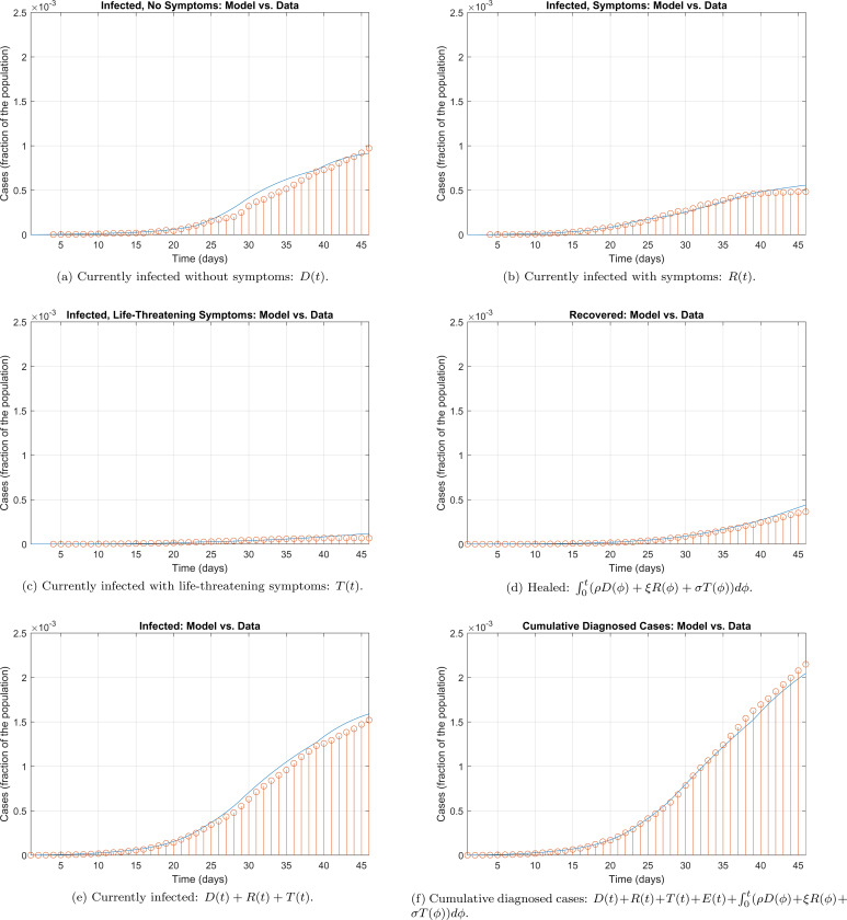
The parameters above were used to simulate the model and generate the graphs reported in Fig. 2. The comparison between the official data and the curves resulting from the SIDARTHE model are provided in Extended Data Fig. 3. The current number of infected (including all stages), the number of recovered and the cumulative number of diagnosed cases are well reproduced, but a small mismatch can be noted in the last days when distinguishing between different SOI. This discrepancy can have two interpretations: on the one hand, the model considers infected with different severities (for example, T(t) is the number of life-threatened patients that would need ICU admission) while the data report the actual treatment that the patients received (for example, the number of patients actually admitted to ICUs, which is constrained by the number of available beds and can be limited if the infected suddenly and quickly worsen, leading to death, before admission to the hospital). Hence, our overestimation of ICU patients may be due to saturation of the healthcare system, which is neglected in the model, or to the sudden worsening of infected who die at home before having the time to reach the ICU. Another possible explanation for our overestimation of patients with symptoms, and life-threatening symptoms, and our underestimation of patients that are asymptomatic or pauci-symptomatic, is that the average age of infected people is getting lower and lower, and younger patients are less likely to show serious or life-threatening symptoms.

Extended Data Fig. 3. Model simulation compared to real data.

Comparison between the official data (red dots histogram) and the results with the calibrated SIDARTHE model (blue line). Panel (a): number of reported infected with no (or mild) symptoms, who are quarantined at home. Panel (b): number of reported infected with symptoms, who are hospitalised. Panel (c): number of reported infected with life-threatening symptoms, admitted to ICU. Panel (d): number of reported recovered individuals. Panel (e): total number of reported infected in all categories. Panel (f): number of cumulative reported cases.

In the possible future scenarios reported in Figs. 3 and 4, the parameters are changed after day 50 as follows. In Fig. 3a,b, α = 0.252, hence R₀ = 0.98 (increased). In Fig. 3c,d, α = 0.105, hence R₀ = 0.50 (significantly decreased). In Fig. 4a,b, ε = 0.400, hence R₀ = 0.59 (decreased, although not as much as in the previous scenario). In Fig. 4c,d, α = 0.420 but also ε = 0.600, therefore R₀ = 0.77 (reduced, although not as much as in the previous two scenarios).

Conversely, Extended Data Fig. 1 shows the epidemic evolution that would have been predicted by the model for the COVID-19 outbreak in Italy if, after day 22, social-distancing countermeasures had been absent (Extended Data Fig. 1a,b), mild (Extended Data Fig. 1c,d), strong (Extended Data Fig. 1e,f) and very strong (Extended Data Fig. 1g,h). In all cases, the actual CFR is ~7.2%, while the perceived CFR is ~9.0%.

Extended Data Fig. 1a,b shows that, in the absence of further countermeasures after day 22 (just closing schools and hygiene recommendations), we have α = 0.422, γ = 0.285 and β = δ = 0.0057, hence R₀ = 1.66 and the model predicts an evolution that leads to 73% of the population having contracted the virus (and ~64% having been diagnosed) and ~5.2% of the population having died because of the contagion over a 300-day horizon (Extended Data Fig. 1a). The peak of the number of concurrently infected individuals occurs at around 76 days and amounts to ~44% of the population; however, the peak of concurrently diagnosed infected individuals occurs later, around 82 days, and amounts to 39% of the population. Extended Data Fig. 1b shows how the different subpopulations of infected individuals evolve over time, and it is interesting to notice that each subpopulation reaches its peak at a different time. In particular, the fraction of infected who need intensive care reaches its peak, almost 16.5% of the population, after 107 days.

Extended Data Fig. 1c,d shows that, with social-distancing countermeasures after day 22 having a mild effect, α = 0.285 and γ = 0.171, hence R₀ = 1.13, still larger than 1. Hence, the peak is delayed (and reduced in amplitude), because the increase in the number of new infected is reduced. Over a 500-day horizon, as shown in Extended Data Fig. 1c, the model predicts an evolution that leads to a peak in the number of concurrently infected individuals around day 170, amounting to 11.7% of the population (10.6% of the population have been diagnosed). Eventually, 35% of the population have contracted the virus (and ~30% have been diagnosed) and ~2.5% of the population have died because of the contagion. The fraction of patients in need of intensive care, as shown in Extended Data Fig. 1d, reaches its peak on day 198, amounting to 5.3% of the population. The adopted social-distancing policy, although mild, has some impact and helps gain more time to strengthen and supply the healthcare system, but is still insufficient.

Extended Data Fig. 1e,f shows that, with stronger social-distancing countermeasures, able to yield α = 0.200 and γ = 0.086, hence R₀ = 0.787, now lower than 1, the peak is not delayed, but anticipated, because the increase in the number of new infected is reduced so much that it soon becomes a decrease. Over a 300-day horizon, as shown in Extended Data Fig. 1e, the model predicts an evolution of the situation that leads to a peak in the number of concurrently infected individuals around day 50, amounting to 0.092% of the population; the peak in diagnosed infected occurs at day 54 and amounts to 0.083% of the population. Eventually, 0.25% of the population have contracted the virus (and ~0.22% have been diagnosed) and ~0.02% of the population have died because of the contagion. The fraction of patients in need of intensive care, as shown in Extended Data Fig. 1f, reaches its peak on day 85, amounting to 0.04% of the population.

Extended Data Fig. 1g,h shows that, with even stronger social-distancing countermeasures, α = γ = 0.057, hence R₀ = 0.0329, significantly lower than 1. Over a 300-day horizon, as shown in Extended Data Fig. 1g, the model predicts an evolution of the situation that leads to a peak in the number of concurrently infected individuals around day 25, amounting to 0.057% of the population; the peak in diagnosed infected occurs at day 35 and amounts to 0.048% of the population. Eventually, 0.086% of the population have contracted the virus (and ~0.074% have been diagnosed) and ~0.006% of the population have died because of the contagion. The fraction of patients in need of intensive care, as shown in Extended Data Fig. 1h, reaches its peak on day 64, amounting to 0.02% of the population.

These scenarios, although surpassed, are fundamental to prove that lockdown was an appropriate policy, given that, in the absence of social-distancing countermeasures, the epidemic could have had tragic outcomes; also, they suggest—for countries early on in the outbreak evolution—that strictly enforcing the lockdown as early as possible leads to enormous benefits with respect to a delayed intervention.

Model sensitivity analysis

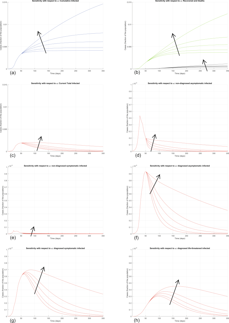
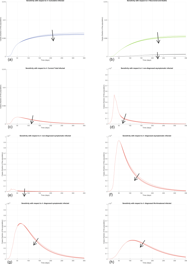
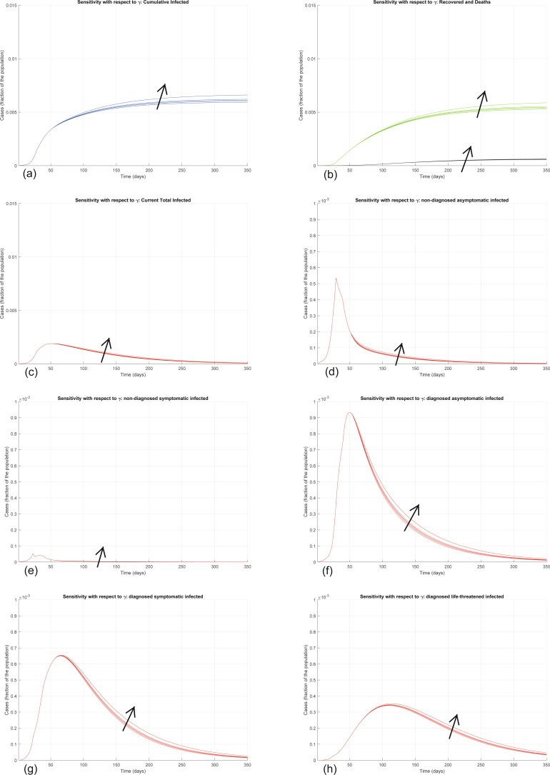
We now investigate the sensitivity of the model to parameter variations, focusing in particular on the parameters that can be influenced by policymakers: transmission parameters, related to lockdown measures (α, β, γ and δ), and testing parameters, related to testing and contact tracing policies (ε, θ). To illustrate the effect of changing the parameter values in the model, our sensitivity analysis results are reported in Extended Data Figs. 4–10.

Extended Data Fig. 4. Sensitivity analysis with respect to α.

Sensitivity analysis showing the effect of varying the transmission coefficient α, whose nominal value is α = 0.21, after day 50. We multiply the nominal value of α by 0.5, 0.8, 1, 1.1, and 1.2, and show the corresponding evolution of the model variables. Panel (a) shows the variation in the total number of cases, panel (b) in the number of recovered individuals (green) and deaths (black), panel (c) in the total number of currently infected individuals, panels (d)–(h) in the number of infected in different categories. Increasing α significantly increases all the curves: the model is extremely sensitive to variations in the value of α.

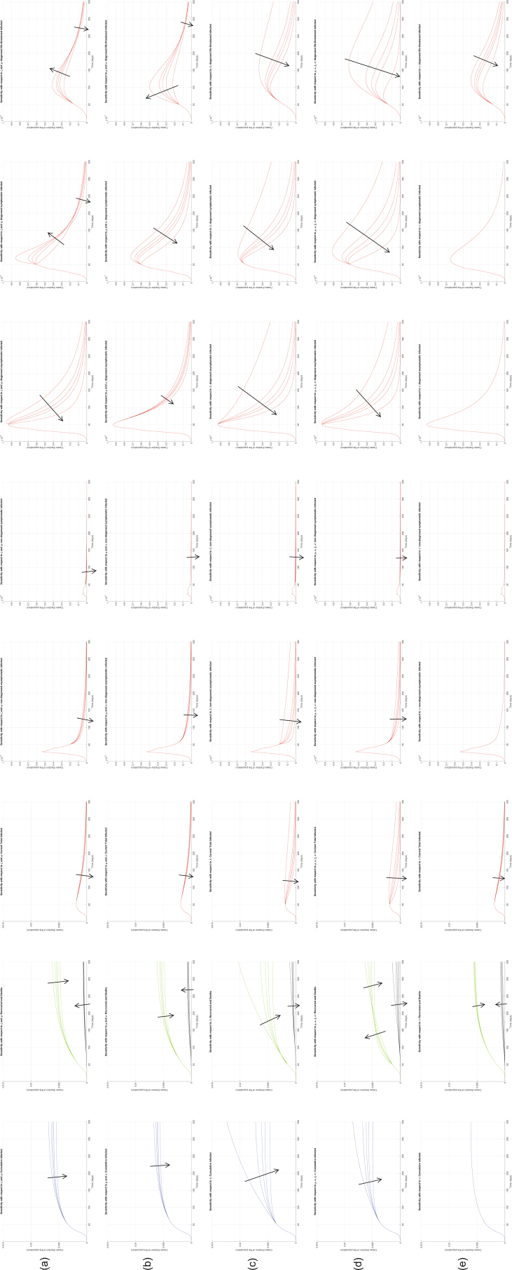
Extended Data Fig. 10. Sensitivity analysis with respect to the other parameters.

Sensitivity analysis showing the effect of varying, after day 50: the worsening coefficients ζ and η leading to clinically relevant symptoms, whose nominal values are ζ = η = 0.0250 (row a); the worsening coefficients μ and ν leading to life-threatening symptoms, whose nominal values are μ = 0.0080 and ν = 0.0150 (row b); the healing coefficient λ, whose nominal value is λ = 0.0800 (row c); the healing coefficients ρ, κ, ξ and σ, whose nominal values are ρ = κ = ξ = 0.0200 and σ = 0.0100 (row d); the mortality coefficient τ, whose nominal value is τ = 0.0100 (row e). In all cases, the nominal value of all the considered parameters is multiplied by 0.5, 0.8, 1, 1.2, 2, and the corresponding evolution of the model variables is shown. Increasing ζ and η decreases the final number of infected and recovered, but also increases the number of deaths; the number of symptomatic and life-threatening infections initially increases, to decrease afterwards. Increasing μ and ν decreases the final number of infected and recovered, but also increases the number of deaths; the number of life-threatening infections initially increases, to decrease afterwards. Increasing λ, as well as the other healing parameters, decreases all the curves, apart from the curve of recovered patients, which initially increases (due to a higher recovery rate) and then eventually decreases (due to less infections overall). Increasing τ leaves all the curves almost unaffected, apart from the curve of life-threatened infected that is decreased, leading to a small decrease in the curve of all infected cases, the curve of recovered that is decreased and the curve of deaths that is increased.

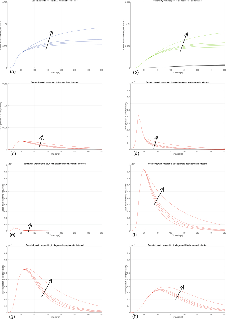
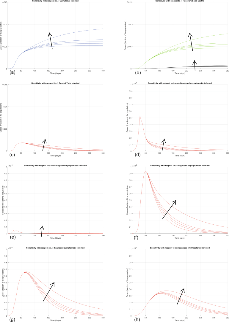
Interestingly, the model is particularly sensitive to variations in the value of α and of ε. Increasing α significantly increases all the curves (Extended Data Fig. 4). Also increasing the other transmission parameters, β, γ and δ, increases all the curves—that is, increases the values of all the variables, point by point, over time (Extended Data Figs. 5–7), although the sensitivity is smaller. All these parameters can be decreased by policymakers, by enforcing lockdown and social-distancing measures, and stringent safety procedures in hospitals and for home assistance of diagnosed infected.

Extended Data Fig. 5. Sensitivity analysis with respect to β.

Sensitivity analysis showing the effect of varying the transmission coefficient β, whose nominal value is β = 0.0050, after day 50. We multiply the nominal value of β by 0.5, 0.8, 1, 1.2, 2, and show the corresponding evolution of the model variables. Panel (a) shows the variation in the total number of cases, panel (b) in the number of recovered individuals (green) and deaths (black), panel (c) in the total number of currently infected individuals, panels (d)–(h) in the number of infected in different categories. Increasing β increases all the curves, although the sensitivity is smaller than with respect to α.

Extended Data Fig. 7. Sensitivity analysis with respect to δ.

Sensitivity analysis showing the effect of varying the transmission coefficient δ, whose nominal value is δ = 0.0050, after day 50. We multiply the nominal value of δ by 0.5, 0.8, 1, 1.2, 2, and show the corresponding evolution of the model variables. Panel (a) shows the variation in the total number of cases, panel (b) in the number of recovered individuals (green) and deaths (black), panel (c) in the total number of currently infected individuals, panels (d)–(h) in the number of infected in different categories. Increasing δ increases all the curves, although the sensitivity is smaller than with respect to α.

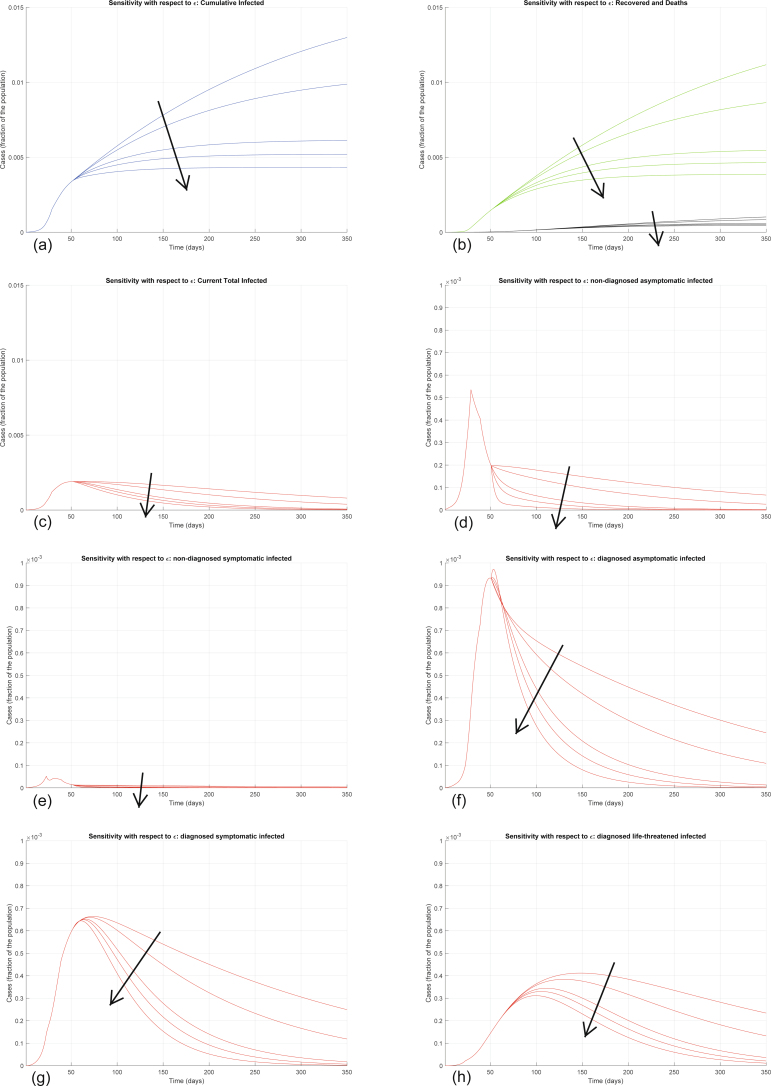
Conversely, increasing ε significantly decreases all the curves (Extended Data Fig. 8). Also increasing the other testing parameter θ decreases all the curves—that is, decreases the values of all the variables, point by point, over time (Extended Data Fig. 9), but the sensitivity is smaller. These two parameters can be increased by policymakers by enforcing population-wide testing and contact tracing, focused on discovering, respectively, asymptomatic and symptomatic infections. Discovering infected people at an earlier stage appears to help reduce the contagion more.

Extended Data Fig. 8. Sensitivity analysis with respect to ε.

Sensitivity analysis showing the effect of varying the testing coefficient ε, whose nominal value is ε = 0.2000, after day 50. We multiply the nominal value of ε by 0.75, 0.8, 1, 1.2, 2, and show the corresponding evolution of the model variables. Panel (a) shows the variation in the total number of cases, panel (b) in the number of recovered individuals (green) and deaths (black), panel (c) in the total number of currently infected individuals, panels (d)–(h) in the number of infected in different categories. Increasing ε significantly decreases all the curves: the model is extremely sensitive to variations in the value of ε.

Extended Data Fig. 9. Sensitivity analysis with respect to θ.

Sensitivity analysis showing the effect of varying the testing coefficient θ, whose nominal value is θ = 0.3705, after day 50. We multiply the nominal value of θ by 0.5, 0.8, 1, 1.2, 2, and show the corresponding evolution of the model variables. Panel (a) shows the variation in the total number of cases, panel (b) in the number of recovered individuals (green) and deaths (black), panel (c) in the total number of currently infected individuals, panels (d)–(h) in the number of infected in different categories. Increasing θ decreases all the curves, but the sensitivity is smaller than with respect to ε.

The other parameters are harder to control with prevention and mitigation strategies (Extended Data Fig. 10). Increasing ζ and η decreases the final number of infected and recovered, but also increases the number of deaths; the number of symptomatic and life-threatening infections initially increases, to decrease afterwards. Increasing μ and ν decreases the final number of infected and recovered, but also increases the number of deaths; the number of life-threatening infections initially increases, to decrease afterwards. Increasing λ, as well as the other healing parameters ρ, κ, ξ and σ, decreases all the curves, apart from the curve of recovered patients, which initially increases (due to a higher recovery rate) and then eventually decreases (due to fewer infections overall). Increasing τ leaves all the curves almost unaffected, apart from the curve of life-threatened infected, which is decreased, also leading to a small decrease in the curve of all infected cases, a decrease in the curve of recovered and an increase in the curve of deaths.

Discussion of the model features

The key feature of our proposed model is the distinction between detected and undetected infection cases, and between cases with different SOI classifications (mild and moderate versus major and extreme). Distinguishing between diagnosed and not diagnosed cases allows us to highlight the perceived distortion in disease statistics, such as the number of infected individuals, the transmission rate and the CFR (the ratio between the number of deaths ascribed to the infection and the number of diagnosed cases). The discrepancy between the actual CFR (total number of deaths due to the infection, divided by the total number of people who have been infected) and the perceived CFR (number of deaths ascribed to the infection, divided by the number of people who have been diagnosed as infected) can be quantified based on this model. Therefore, the model can explain the possible discrepancy between the actual infection dynamics and the perception of the phenomenon. Misperception (either resulting in underestimating or overestimating) can be particularly relevant in the early phases of an epidemic phenomenon due to the lack of thorough information: for example, performing an insufficient number of tests may lead to underestimating the transmission rate (because many infected subjects are not diagnosed as such) and overestimating the CFR (because critical or fatal cases hardly go undetected). The model thus provides a rough quantification of the error in estimating the actual number of infected people due to the lack of proper diagnostic tests, or due to insufficient number of diagnostic tests being performed. Also, it can explain and predict the long-term effects of underdiagnosis, including the (apparently surprising) increased number of infections and fatalities, with sudden outbreaks after long silent periods.

Once the model parameters have been estimated on the basis of the available clinical data, the model enables us to reproduce and predict the dynamic evolution of the epidemic and to evaluate the possible underestimation or overestimation of the epidemic phenomenon based on current statistics, which are heavily subject to bias (for example, asymptomatic patients may get tested according to some protocols, not tested according to others).

The model helps evaluate and predict the effect of the implementation of different guidelines and protocols (for example, more extensive screening for the disease or stricter social-distancing measures), which typically results in a change in the model parameters.

The model predictions in the long run are not very sensitive to the initial conditions, but they are sensitive to the parameter values (and in particular extremely sensitive to some of these, as our sensitivity analysis has indicated), which are deeply uncertain and can vary due to several factors, such as population density, cultural habits, environmental conditions and age distribution of the population. The predictions must also consider parameter variations due to the measures imposed by the government. This is a fundamental aspect: in the long term, not imposing drastic measures leads to catastrophic outcomes, even when the initially affected population is a small fraction.

Social-distancing measures are modeled by reducing the infection coefficients α, β, γ and δ. The infection peak time is not monotonic with increasing restrictions. Partial restrictions on population movements postpone the peak, while strong restrictions anticipate the peak. Mild containment measures may have negative effects, for example augmenting the fraction of the population with life-threatening symptoms with respect to the fraction of population with mild symptoms.

Diagnosis campaigns can reduce the infection peak, because the diagnosed population enters quarantine and hence is less likely to affect the susceptible population.

Reporting Summary

Further information on research design is available in the Nature Research Reporting Summary linked to this article.

Online content

Any methods, additional references, Nature Research reporting summaries, source data, extended data, supplementary information, acknowledgements, peer review information; details of author contributions and competing interests; and statements of data and code availability are available at 10.1038/s41591-020-0883-7.

Extended data

Extended Data Fig. 6. Sensitivity analysis with respect to γ.

Sensitivity analysis showing the effect of varying the transmission coefficient γ, whose nominal value is γ = 0.11, after day 50. We multiply the nominal value of γ by 0.5, 0.8, 1, 1.2, 2, and show the corresponding evolution of the model variables. Panel (a) shows the variation in the total number of cases, panel (b) in the number of recovered individuals (green) and deaths (black), panel (c) in the total number of currently infected individuals, panels (d)–(h) in the number of infected in different categories. Increasing γ increases all the curves, although the sensitivity is smaller than with respect to α and β.

Author contributions

G.G., F.B. and P.C. proposed the model and performed the mathematical derivations, the fitting and the simulations. R.B., A.D.F., A.D.M. and M.C. provided first-hand insight into the disease evolution and provided the clinical contextualization and interpretation of the results. All authors wrote and approved the manuscript.

Data availability

We gathered epidemiological data from the following publicly available data sources: Italian Civil Protection (http://www.protezionecivilfor exampleov.it/media-comunicazione/comunicati-stampa) and the Ministry of Health (http://www.salutfor exampleov.it/portale/home.html). All the epidemiological information we used is documented in the Extended Data and Supplementary Tables. Raw data are reported in Supplementary Table 1 and are also included in Extended Data Fig. 3.

Code availability

The codes are available at http://users.dimi.uniud.it/~giulia.giordano/docs/papers/SIDARTHEcode.zip.

Competing interests

The authors declare no competing interests.

Extended data

is available for this paper at 10.1038/s41591-020-0883-7.

Supplementary information

is available for this paper at 10.1038/s41591-020-0883-7.

References

- 1.Velavan TP, Meyer CG. The COVID-19 epidemic. Trop. Med. Int. Health. 2020;25:278–280. doi: 10.1111/tmi.13383. [DOI] [PMC free article] [PubMed] [Google Scholar]
- 2.Wu Z, McGoogan JM. Characteristics of and important lessons from the coronavirus disease 2019 (COVID-19) outbreak in China: summary of a report of 72,314 cases from the Chinese center for disease control and prevention. JAMA. 2020;323:1239–1242. doi: 10.1001/jama.2020.2648. [DOI] [PubMed] [Google Scholar]
- 3.Guan, W.-J.et al. Clinical characteristics of coronavirus disease 2019 in China. N. Engl. J. Med.10.1056/NEJMoa2002032 (2020). [DOI] [PMC free article] [PubMed]
- 4.WHO. Coronavirus Disease 2019 (COVID-19): Situation Report 76 (WHO, 2020).
- 5.Remuzzi A, Remuzzi G. COVID-19 and Italy: what next? Lancet Health Policy. 2020;395:1225–1228. doi: 10.1016/S0140-6736(20)30627-9. [DOI] [PMC free article] [PubMed] [Google Scholar]
- 6.Giuffrida, A. & Beaumont, P. Coronavirus: inquiry opens into hospitals at centre of Italy outbreak. The Guardian (26 February 2020).
- 7.Ministero della Salute (Italian Ministry of Health). http://www.salute.gov.it/imgs/C_17_notizie_4403_0_file.pdf (5 April 2020).
- 8.Italian Civil Protection. Situazione Italia al 5 marzo. http://www.salute.gov.it/portale/nuovocoronavirus/dettaglioNotizieNuovoCoronavirus.jsp?lingua=italiano&menu=notizie&p=dalministero&id=4157 (5 March 2020).
- 9.Chronology of main steps and legal acts taken by the Italian Government for the containment of the COVID-19 epidemiological emergency. http://www.protezionecivile.gov.it/documents/20182/1227694/Summary+of+measures+taken+against+the+spread+of+C-19/c16459ad-4e52-4e90-90f3-c6a2b30c17eb (accessed 12 March 2020).
- 10.Wang Y, Wang Y, Chen Y, Quin Q. Unique epidemiological and clinical features of the emerging 2019 novel coronavirus pneumonia (COVID-19) implicate special control measures. J. Med. Virol. 2020;92:568–576. doi: 10.1002/jmv.25748. [DOI] [PMC free article] [PubMed] [Google Scholar]
- 11.Fisman, D., Rivers, C., Lofgren, E. & Majumder, M. S. Estimation of MERS-Coronavirus reproductive number and case fatality rate for the Spring 2014 Saudi Arabia outbreak: insights from publicly available data. PLoS Curr.10.1371/currents.outbreaks.98d2f8f3382d84f390736cd5f5fe133c (2014). [DOI] [PMC free article] [PubMed]
- 12.Zhao S, et al. Preliminary estimation of the basic reproduction number of novel coronavirus (2019-nCoV) in China, from 2019 to 2020: a data-driven analysis in the early phase of the outbreak. Int. J. Inf. Dis. 2020;92:214–217. doi: 10.1016/j.ijid.2020.01.050. [DOI] [PMC free article] [PubMed] [Google Scholar]
- 13.Read, J., Bridgen, J. R., Cummings, D. A. T., Ho, A. & Jewell, C. P. Novel coronavirus 2019-nCoV: early estimation of epidemiological parameters and epidemic predictions. Preprint at medRxiv10.1101/2020.01.23.20018549 (2020). [DOI] [PMC free article] [PubMed]
- 14.Zou L, et al. SARS-CoV-2 viral load in upper respiratory specimens of infected patients. N. Engl. J. Med. 2020;382:1177–1179. doi: 10.1056/NEJMc2001737. [DOI] [PMC free article] [PubMed] [Google Scholar]
- 15.Anderson, R. M. & May, R. M. Infectious Diseases of Humans (Oxford Univ. Press, 1991).
- 16.Diekmann, O. & Heesterbeek, J. A. P. Mathematical Epidemiology of Infectious Diseases: Model Building, Analysis and Interpretation (Wiley, 2000).
- 17.Hethcote HW. The mathematics of infectious diseases. SIAM Rev. 2000;42:599–653. doi: 10.1137/S0036144500371907. [DOI] [Google Scholar]
- 18.Brauer, F. & Castillo-Chavez, C. Mathematical Models in Population Biology and Epidemiology 2nd edn (Springer, 2012).
- 19.Kermack WO, McKendrick AG. A contribution to the mathematical theory of epidemics. Proc. R. Soc. Lond. 1927;115:700–721. [Google Scholar]
- 20.Lin Q, et al. A conceptual model for the coronavirus disease 2019 (COVID-19) outbreak in Wuhan, China with individual reaction and governmental action. Int. J. Inf. Dis. 2020;93:211–216. doi: 10.1016/j.ijid.2020.02.058. [DOI] [PMC free article] [PubMed] [Google Scholar]
- 21.Anastassopoulou C, Russo L, Tsakris A, Siettos C. Data-based analysis, modelling and forecasting of the COVID-19 outbreak. PLoS One. 2020;15:e0230405. doi: 10.1371/journal.pone.0230405. [DOI] [PMC free article] [PubMed] [Google Scholar]
- 22.Casella, F. Can the COVID-19 epidemic be managed on the basis of daily data? Preprint at https://arxiv.org/abs/2003.06967 (2020).
- 23.Wu J, et al. Estimating clinical severity of COVID-19 from the transmission dynamics in Wuhan, China. Nat. Med. 2020;26:506–510. doi: 10.1038/s41591-020-0822-7. [DOI] [PMC free article] [PubMed] [Google Scholar]
- 24.Hellewell J, et al. Feasibility of controlling COVID-19 outbreaks by isolation of cases and contacts. Lancet Global Health. 2020;8:e488–e496. doi: 10.1016/S2214-109X(20)30074-7. [DOI] [PMC free article] [PubMed] [Google Scholar]
- 25.Kucharski, A. J. et al. Early dynamics of transmission and control of COVID-19: a mathematical modelling study. Lancet Global Health10.1016/S1473-3099(20)30144-4 (2020). [DOI] [PMC free article] [PubMed]
- 26.Gumel, A. B. et al. Modelling strategies for controlling SARS outbreaks. Proc. R. Soc. B Biol. Sci. 10.1098/rspb.2004.2800 (2004). [DOI] [PMC free article] [PubMed]
- 27.Lan, L. et al. Positive RT-PCR test results in patients recovered from COVID-19. JAMA10.1001/jama.2020.2783 (2020). [DOI] [PMC free article] [PubMed]
- 28.Peto J. Covid-19 mass testing facilities could end the epidemic rapidly. Br. Med. J. 2020;368:m1163. doi: 10.1136/bmj.m1163. [DOI] [PubMed] [Google Scholar]
- 29.Corman VM, et al. Detection of 2019 novel coronavirus (2019-nCoV) by real-time RT-PCR. Euro Surveill. 2020;25:2000045. doi: 10.2807/1560-7917.ES.2020.25.3.2000045. [DOI] [PMC free article] [PubMed] [Google Scholar]
- 30.Li, Z. et al. Development and clinical application of a rapid IgM-IgG combined antibody test for SARS-CoV-2 infection diagnosis. J. Med. Virol. 10.1002/jmv.25727 (2020). [DOI] [PMC free article] [PubMed]
- 31.Roosa K, et al. Short-term forecasts of the COVID-19 epidemic in Guangdong and Zhejiang, China: February 13–23, 2020. J. Clin. Med. 2020;9:E596. doi: 10.3390/jcm9020596. [DOI] [PMC free article] [PubMed] [Google Scholar]
- 32.Wang C, et al. Risk management of COVID-19 by universities in China. J. Risk Financ. Manag. 2020;13:36. doi: 10.3390/jrfm13020036. [DOI] [Google Scholar]
- 33.Ji Y, Ma Z, Peppelenbosch MP, Pan Q. Potential association between COVID-19 mortality and health-care resource availability. Lancet Global Health. 2020;8:e480. doi: 10.1016/S2214-109X(20)30068-1. [DOI] [PMC free article] [PubMed] [Google Scholar]
- 34.Wang M, et al. Remdesivir and chloroquine effectively inhibit the recently emerged novel coronavirus (2019-nCoV) in vitro. Cell Res. 2020;30:269–271. doi: 10.1038/s41422-020-0282-0. [DOI] [PMC free article] [PubMed] [Google Scholar]
- 35.Chang, Y.-C. et al. Potential therapeutic agents for COVID-19 based on the analysis of protease and RNA polymerase docking. Preprint at Preprintshttps://www.preprints.org/manuscript/202002.0242/v1
- 36.Diao, B. et al. Reduction and functional exhaustion of T cells in patients with coronavirus disease 2019 (COVID-19). Preprint at medRxiv10.1101/2020.02.18.20024364 (2020). [DOI] [PMC free article] [PubMed]
- 37.Chen, W.-H., Strych, U., Hotez, P. J. & Bottazzi, M. E. The SARS-CoV-2 vaccine pipeline: an overview. Curr. Trop. Med. Rep.10.1007/s40475-020-00201-6 (2020). [DOI] [PMC free article] [PubMed]
- 38.Epidemiologist: ‘Too early to say’ if infected people develop immunity from the coronavirus (interview to David Heymann). The Hillhttps://thehill.com/policy/healthcare/490059-epidemiologist-too-early-to-say-if-infected-people-develop-immunity-from (29 March 2020).
- 39.Chen D, et al. Recurrence of positive SARS-CoV-2 RNA in COVID-19: a case report. Int. J. Infect. Dis. 2020;93:297–299. doi: 10.1016/j.ijid.2020.03.003. [DOI] [PMC free article] [PubMed] [Google Scholar]
- 40.Zhou L, et al. Cause analysis and treatment strategies of ‘recurrence’ with novel coronavirus pneumonia (covid-19) patients after discharge from hospital. Zhonghua Jie He He Hu Xi Za Zhi. 2020;43:E028. doi: 10.3760/cma.j.cn112147-20200229-00219. [DOI] [PubMed] [Google Scholar]
- 41.Houser KV, et al. Enhanced inflammation in New Zealand white rabbits when MERS-CoV reinfection occurs in the absence of neutralizing antibody. PLoS Pathog. 2017;13:e1006565. doi: 10.1371/journal.ppat.1006565. [DOI] [PMC free article] [PubMed] [Google Scholar]
- 42.Hemida MG, et al. Longitudinal study of middle east respiratory syndrome coronavirus infection in dromedary camel herds in Saudi Arabia, 2014–2015. Emerg. Microbes Infect. 2017;6:e56. doi: 10.1038/emi.2017.44. [DOI] [PMC free article] [PubMed] [Google Scholar]
- 43.Subbarao K, et al. Prior infection and passive transfer of neutralizing antibody prevent replication of severe acute respiratory syndrome coronavirus in the respiratory tract of mice. J. Virol. 2004;78:3572–3577. doi: 10.1128/JVI.78.7.3572-3577.2004. [DOI] [PMC free article] [PubMed] [Google Scholar]
- 44.Ji, N.-L. et al. Clinical features of pediatric patients with COVID-19: a report of two family cluster cases. World J. Pediatr.10.1007/s12519-020-00356-2 (2020). [DOI] [PMC free article] [PubMed]
- 45.Qian, G. et al. A COVID-19 transmission within a family cluster by presymptomatic infectors in China. Clin. Infect. Dis. 10.1093/cid/ciaa316 (2020). [DOI] [PMC free article] [PubMed]
- 46.Fineberg, H. V. Ten weeks to crush the curve. N. Engl. J. Med. 10.1056/NEJMe2007263 (2020). [DOI] [PubMed]
- 47.Istituto Superiore di Sanità. Recommendations for People in Family Isolation and Their Caregivershttp://www.salutfor exampleov.it/portale/nuovocoronavirus/dettaglioNotizieNuovoCoronavirus.jsp?lingua=italiano&menu=notizie&p=dalministero&id=4266 (accessed 4 April 2020).
- 48.Pung R, et al. Investigation of three clusters of COVID-19 in Singapore: implications for surveillance and response measures. Lancet. 2020;395:1039–1046. doi: 10.1016/S0140-6736(20)30528-6. [DOI] [PMC free article] [PubMed] [Google Scholar]
- 49.Rothe C, et al. Transmission of 2019-nCoV infection from an asymptomatic contact in Germany. N. Engl. J. Med. 2020;382:970–971. doi: 10.1056/NEJMc2001468. [DOI] [PMC free article] [PubMed] [Google Scholar]
- 50.Kimball A, et al. Asymptomatic and presymptomatic SARS-CoV-2 infections in residents of a long-term care skilled nursing facility. King County, Washington, March 2020. Morb. Mortal Wkly Rep. 2020;69:377–381. doi: 10.15585/mmwr.mm6913e1. [DOI] [PMC free article] [PubMed] [Google Scholar]
- 51.Nishiura H, Linton NM, Akhmetzhanov AR. Serial interval of novel coronavirus (COVID-19) infections. Int. J. Infect. Dis. 2020;93:284–286. doi: 10.1016/j.ijid.2020.02.060. [DOI] [PMC free article] [PubMed] [Google Scholar]
- 52.Du Z, et al. Serial interval of COVID-19 among publicly reported confirmed cases. Emerg. Infect. Dis. 2020;26:6. doi: 10.3201/eid2606.200357. [DOI] [PMC free article] [PubMed] [Google Scholar]
- 53.King AA, et al. Avoidable errors in the modelling of outbreaks of emerging pathogens, with special reference to Ebola. Proc. Biol. Sci. 2015;282:20150347. doi: 10.1098/rspb.2015.0347. [DOI] [PMC free article] [PubMed] [Google Scholar]
- 54.Dowd, J. B. et al. Demographic science aids in understanding the spread and fatality rates of COVID-19. OSFhttps://osf.io/fd4rh (2020). [DOI] [PMC free article] [PubMed]
- 55.Istituto Superiore di Sanità. Characteristics of COVID-19 patients dying in Italy. https://www.epicentro.iss.it/en/coronavirus/sars-cov-2-analysis-of-deaths (2020).
Associated Data
This section collects any data citations, data availability statements, or supplementary materials included in this article.
Supplementary Materials
Supplementary Table 1.
Data Availability Statement