A U-statistics for integrative analysis of multilayer omics data

Abstract

Motivation

The emerging multilayer omics data provide unprecedented opportunities for detecting biomarkers that are associated with complex diseases at various molecular levels. However, the high-dimensionality of multiomics data and the complex disease etiologies have brought tremendous analytical challenges.

Results

We developed a U-statistics-based non-parametric framework for the association analysis of multilayer omics data, where consensus and permutation-based weighting schemes are developed to account for various types of disease models. Our proposed method is flexible for analyzing different types of outcomes as it makes no assumptions about their distributions. Moreover, it explicitly accounts for various types of underlying disease models through weighting schemes and thus provides robust performance against them. Through extensive simulations and the application to dataset obtained from the Alzheimer’s Disease Neuroimaging Initiatives, we demonstrated that our method outperformed the commonly used kernel regression-based methods.

Availability and implementation

The R-package is available at https://github.com/YaluWen/Uomic.

Supplementary information

Supplementary data are available at Bioinformatics online.

1 Introduction

Benefiting from high-throughput biotechnologies, large amount of multilayer omics data have been collected and they hold great promise in systematically investigating the etiologies of complex human diseases at different molecular levels (e.g. genomics, transcriptomics and epigenomics) (Ashley, 2015). While traditionally the association studies are conducted between complex diseases and single-layer omics data (e.g. genetic variants, DNA methylation markers and gene expression levels), such a strategy only uses partial information from one layer of omics data and thus can result in suboptimal performance, especially when multilayer omics data jointly explain the disease variations. Moreover, for many complex diseases, only a small proportion of disease heritability can be explained by single-layer omics data (e.g. genetic data) (Manolio et al., 2009), and the variants identified from different studies may suffer from poor reproducibility (Phan et al., 2012). Therefore, an integrative approach that can make use of information from all layers of omics data has the potential to identify new disease-associated biomarkers and provide better insights into disease mechanisms (do Valle et al., 2018).

Comprehensive reviews of integrative analysis on multilayer omics data are summarized in Bersanelli et al. (2016), Li et al. (2018) and Zeng and Lumley (2018). Existing association testing approaches are usually based on kernel machine regressions (KMRs) that are widely used in genome-wide association studies (GWAS) (Huang et al., 2014; Yan et al., 2019; Zhao et al., 2014, 2018). At the core, KMR assumes that individuals with similar profiles at the molecular levels have similar outcomes if these molecular features and the outcomes are associated. For GWAS, KMR measures genetic similarities using a kernel function, and builds a score-type of statistics that asymptotically follows a mixture of ${\chi }^2$ distribution under the null hypothesis (Lee et al., 2012; Wu et al., 2010, 2011). For multilayer omics data analysis, KMR extends the idea used in GWAS by replacing the genetic similarities to similarities determined from all layers of omics data using various kernel functions (Huang, 2014; Huang et al., 2014; Zhao et al., 2014, 2018). For example, Huang et al. estimated omics-similarities as a weighted average of similarities derived from each layer of omics data using a linear kernel, and the weights were determined empirically so that each layer of omics data contributed approximately equally to the overall score-type of statistics (Huang et al., 2014). Zhao et al. used a similar KMR framework for the integrative analysis of genome-wide methylation and genomic data, where a composite kernel was built as a weighted average of genomic and methylation similarities. The statistical significance was evaluated through a projection approach, where a kernel principal component analysis (KPCA) was used to make the genomic and methylation similarities orthogonal. The overall score-type of statistics can be viewed as a weighted mixture of independent ${\chi }^2$, and thus P-values can be computed analytically (Zhao et al., 2018). Although the score-type of statistics used in these KMR-based methods are in quadratic forms and have attractive properties under many scenarios (Huang et al., 2014; Yan et al., 2019; Zhao et al., 2014, 2018), most of these methods are parametric/semiparametric and assume the outcomes come from the exponential family that may not hold in practice. For example, the distribution of cognitive test scores in the Alzheimer’s Disease Neuroimaging Initiatives (ADNI) dataset may not come from the exponential family (Supplementary Fig. S1). When the distributional assumption is violated, these KMR methods can be subject to low power and/or high type I error. Many efforts have been made to improve the robustness of statistical modeling (Wu and Ma, 2015). For example, robust loss functions (e.g. least absolute deviation, exponential squared and rank-based losses) have been developed for regression models. While these strategies are important for biomedical research, they are not directly applicable for association studies with multiomics data.

When integrating multilayer omics data for association studies, selecting relevant layers of omics data is of great importance and an extensive review on variable selection for multiomics data integration can be found at Wu et al. Indeed, in practice it is quite likely that only some layers of omics data are associated with the outcome of interest (Wu et al., 2019; Yan et al., 2019; Zhao et al., 2018). Building the score-type of statistics with similarities estimated from all layers of omics data may lead to suboptimal performance, especially when only a few layers are associated with the outcomes. To obtain optimal power, several strategies have been proposed. One of them focuses on selecting only disease-associated layers of omics data for the association analysis through the projection of multiomics data into orthogonal subspaces (Zhao et al., 2018). For example, Zhao et al. proposed to project multiomics data into orthogonal subspaces so that they are independent of each other. P-values for the associations between each combination of multilayer omics data in the subspaces and the outcome were obtained, and the optimal test statistics was built through a minimum P-value approach (Zhao et al., 2018). While this projection-based method can obtain the asymptotic distribution of the test statistics without relying on resampling techniques, it can have suboptimal performance when different layers of omics data are highly correlated. Another strategy is to view the association testing as a problem of combining multiple correlated P-values, which are obtained from different combinations of multilayer omics data in the original space (Poole et al., 2016; Yan et al., 2019). While this strategy has potential to capture the inter-relationships among different layers of omics data, it relies on resampling techniques to estimate correlations between P-values and can be computationally demanding. Moreover, it focuses on the correlations between P-values (i.e. at the summary statistics level), and thus may not fully capture the relationships among multiomics data and overlook the consensus information embedded in them.

To address these limitations, we propose a flexible U-statistics-based non-parametric framework for association analysis on multilayer omics data (Shieh, 1997), where two strategies are developed to obtain optimal power of the test. Our proposed method makes no assumption about the distribution of the outcomes, and thus can provide a robust and powerful tool for analyzing various types of outcomes. Moreover, our method can account for all possible disease models (e.g. for genomic and gene expression data, there are three possible disease models: only gene expression is related; only genetic data is associated and both gene expression and genetic data are related), and thus provide a unified framework for diseases with various underlying causes. In the following sections, we first lay out the details of our proposed method and its theoretical properties, and then evaluate its performance through extensive simulation studies. Finally, we perform an integrative analysis on the DNA sequencing and gene expression data obtained from the ADNI (Saykin et al., 2010).

2 Materials and methods

Suppose that data are collected on n independent subjects with continuous or discrete outcomes $(y_1,y_2,\dots ,y_n)$. Similar to many existing methods (Yan et al., 2019; Zhao et al., 2014, 2018), we assume that omics data are grouped into genes based on some prior biological information. Let ${\mathit{O}}_i$ be a $n\times p_i$ matrix denoting the ith layer of omics data, where p_i is the number of variants for the ith layer. We use $\mathit{O}=({\mathit{O}}_1,{\mathit{O}}_2,\dots ,{\mathit{O}}_{n_{\mathrm{o}}})$ to denote all n_o layers of omics data.

2.1 Motivation from a KMR model used for association analysis of single-layer omics data

To motivate the idea of our method, we first overview the widely used KMR models for association analysis of single-layer omics data. Without loss of generality, we present KMR for genetic association analysis. KMR relates the outcomes to genotypes via a semiparametric KMR model as

$$g(E(\mathit{y}))=\mathit{X}\mathit{\beta }+h({\mathit{O}}_{\mathrm{g}}),$$ (1)

where $g(·)$ is a link function, $\mathit{\beta }$ are regression coefficients for covariates $\mathit{X}$ (e.g. age and gender), ${\mathit{O}}_{\mathrm{g}}$ is a $n\times p_{\mathrm{g}}$ matrix of genotypes with ${\mathit{O}}_{\mathrm{g}}^i$ being the genetic variants for individual i and $h(·)$ is a function of joint effects of p_g genetic variants on the outcome.

Under the KMR framework, $h(·)$ is a function in a Reproducing Kernel Hilbert Space generated by some kernel function $K(·,·)$. The kernel matrix $\mathit{K}={({\kappa }_{i,j})}_{n\times n}$ with the (i, j)th element being ${\kappa }_{i,j}=K({\mathit{O}}_{\mathrm{g}}^i,{\mathit{O}}_{\mathrm{g}}^j)$ measures the genetic similarity between ith and jth individuals. Using the connections between KMR and generalized linear mixed model (Wu et al., 2010, 2011), hypothesis testing can be conducted via a variance component score test as

$$Q=(\mathit{y}-{\widehat{\mathit{y}}}_0)\prime \mathit{K}(\mathit{y}-{\widehat{\mathit{y}}}_0),$$ (2)

where ${\widehat{\mathit{y}}}_0$ are the estimates of $\mathit{y}$ under the null hypothesis. Q asymptotically follows a mixture of ${\chi }^2$ distribution under the null hypothesis (Wu et al., 2010, 2011), and it can be partitioned into two parts as

$$Q=\sum _{i\ne j}(y_i-{\widehat{y}}_i)(y_j-{\widehat{y}}_j){\kappa }_{i,j}+\sum _i{(y_i-{\widehat{y}}_i)}^2{\kappa }_{i,i},$$ (3)

where the first term is closed related to the test statistics introduced in this work.

2.2 A U-statistics method for association analysis on multilayer omics data

The basic idea in KMR for association analysis of single-layer omics data is that similarities in omics data can lead to outcome similarities if the specific layer of omics data is associated with the outcomes. Similar idea can be adopted in multilayer omics data analysis, where similarities derived from single-layer omics data are replaced by those calculated from all layers of omics data. While promising, KMRs usually assume that outcomes come from an exponential family and can be subject to lower power if this assumption is not met. Here, we develop a U-statistics-based method that can consider outcomes with various distributions and utilize information from all layers of omics data for association testing.

Let $\mathit{X}$ be an n × p matrix representing p demographic variables (e.g. age and gender). Define ${\mathit{P}}_0={\mathit{I}}_n-\mathit{X}{({\mathit{X}}^{\prime }\mathit{X})}^{-1}\mathit{X}\prime$ and ${\mathit{e}}_n=({ϵ}_1,{ϵ}_2,\dots ,{ϵ}_n)\prime ={\mathit{P}}_0\mathit{y}$, where ${\mathit{e}}_n$ can be viewed as residuals after adjusting for the effects of covariates $\mathit{X}$. Indeed, when the outcomes are normally distributed, ${\mathit{e}}_n$ are the residuals from a simple linear regression model under the null. We define R_i as the rank of residuals for the ith subject (i.e. $R_i=\text{rank}({ϵ}_i)$), and further define a rank-based kernel function that is robust to different distributions of the outcomes as

$$h(R_i,R_j)=\frac{(R_i-{\mu }_R)(R_j-{\mu }_R)}{{\sigma }_R^2},$$ (4)

where ${\mu }_R=E(R)$ and ${\sigma }_R^2=\text{var}(R)$. It is straightforward to show this kernel function has finite second-moment ($E\left[h^2(R_i,R_j)\right]<\infty$) and is degenerate ($\text{var}\left(h_1(R_1)\right)=0$ with $h_1(r_1)=E\left[h(r_1,R_2)\right]$). When there are no covariates to adjust for, R_i is simply the rank of the outcome values for the ith subject. Let $\mathit{K}={({\kappa }_{i,j})}_{n\times n}$ represent pairwise similarity matrix that are derived from all omics data. Using the same idea used in genetic association testing (Wei et al., 2016), we define our test statistics as

$$U_{\text{omic}}=\sum _{i=1}^n\sum _{j\ne i}{\kappa }_{i,j}h(R_i,R_j).$$ (5)

The kernel function $h(R_i,R_j)$ can be viewed as a covariate-adjusted rank-based outcome similarity between the ith and jth subjects. If two individuals have similar outcomes (or adjusted-outcomes), we would expect their ranks are similar and thus a higher rank-based outcome similarity. The test statistics is a weighted summation of all pairwise rank-based outcome similarities, where the weights are omics-similarities determined from all layers of omics data. Under the null hypothesis where none of the omics data is related to the outcomes, the rank-based outcome similarities are not associated with omic-similarities. Therefore, U_omic is expected to be zero as $E\left[h(R_i,R_j)\right]=0$. Under the alternatives (i.e. at least one layer of omics data are related to the outcomes), the rank-based outcome similarities increase as the omics-similarities increase, and thus a positive U_omic is expected.

2.3 Asymptotic distribution of the test statistics

The asymptotic distributions for U-statistics have been well established in the existing literature (Hoeffding, 1948; Shieh, 1997). The limiting distribution is a normal distribution when the kernel function in non-degenerate (Hoeffding, 1948), and it is a mixture of ${\chi }^2$ when the kernel function is degenerate (Shieh, 1997). The proposed test statistics in Equation (5) can be viewed as a weighted U-statistics with a degenerate kernel function as $\text{var}(E(h(R_i,R_j)|R_i))=0$.

Let $\gamma =({\mu }_R,{\sigma }_R)$, and we use ${\gamma }_0=({\mu }_0,{\sigma }_0)$ to represent the true values of γ. Given the assumptions listed in Supplementary A1, under the null hypothesis, we have

$$U_{\text{omic}}({\gamma }_0)\sim \sum _m{\eta }_m{\chi }_1^2,$$

where η_m is the mth eigenvalue of $\mathit{K}$. Recall $\mathit{K}={({\kappa }_{i,j})}_{n\times n}$ denotes the weight matrix, and it is symmetric with diagonal values being zeros. There exists an orthogonal matrix $\mathit{B}=(b_{im})$ such that $\mathit{BKB}\prime =\mathbf{\Lambda }$, where $\mathbf{\Lambda }=\text{diag}({\eta }_m)$. It is straightforward to see that

$$\begin{array}{c}{U}_{\text{omic}}({\gamma }_0)=\sum _i\sum _{j\ne i}\sum _m{\eta }_m{b}_{im}{b}_{jm}\frac{(R_i-{\mu }_0)(R_j-{\mu }_0)}{{\sigma }_0^2}\\ =\sum _m{\eta }_m\sum _i\sum _j{b}_{im}{b}_{jm}\frac{R_i-{\mu }_0}{{\sigma }_0}\frac{R_j-{\mu }_0}{{\sigma }_0}\\ =\sum _m{\eta }_m{\left(\sum _i{b}_{im}\frac{R_i-{\mu }_0}{{\sigma }_0}\right)}^2\sim \sum _m{\eta }_m{\chi }_1^2.\end{array}$$ (6)

In practice, the true parameter γ₀ is unknown in advance. As we propose to directly work with rank-based statistics, the parameters only depend on the sample size and how many ties are present. We estimated $\widehat{\gamma }$ using ${\widehat{\mu }}_R=n+1/2$ and ${\widehat{\sigma }}_R^2=(\mathit{R}-{\widehat{\mu }}_R)\prime (\mathit{R}-{\widehat{\mu }}_R)/n-1$. Note, ${\widehat{\sigma }}_R^2=n(n+1)/12$, when there are no ties. Under the null hypothesis, we have

$$U_{\text{omic}}(\widehat{\gamma })\sim \sum _m\eta {\prime }_m{\chi }_1^2,$$

where $\eta {\prime }_m$ are the eigenvalues of matrix $({\mathit{I}}_n-(1/n\left){\mathbf{1}}_{n\times n}\right)\mathit{K}({\mathit{I}}_n-(\mathbf{1}/n\left){\mathbf{1}}_{n\times n}\right)$ with all elements in ${\mathbf{1}}_{n\times n}$ being 1. Using the same idea in Shieh (1997), $U_{\text{omic}}(\widehat{\gamma })$ can be approximated as

$${\tilde{U}}_{\text{omic}}(\widehat{\gamma })=\sum _m{\eta }_m{\left\{\sum _i{b}_{im}\left(\frac{R_i-{\mu }_0}{{\sigma }_0}+\left(\frac{\partial E_{{\gamma }_0}\left[R_i-\mu /\sigma \right]}{\partial \gamma }{|}_{\gamma ={\gamma }_0}\right)(\widehat{\gamma }-{\gamma }_0)\prime \right)\right\}}^2,$$

where $E_{{\gamma }_0}\left[R_i-\mu /\sigma \right]$ denotes the expectation of $R_i-\mu /\sigma$ when the $E(R_i)={\mu }_0$. We can show that ${\tilde{U}}_{\text{omic}}(\widehat{\gamma })\sim {\sum }_m\eta {\prime }_m{\chi }_1^2$. As $\widehat{\gamma }{\to }_P{\gamma }_0$, we can also show that ${\tilde{U}}_{\text{omic}}(\widehat{\gamma })-U_{\text{omic}}(\widehat{\gamma }){\to }_{P}0$. Therefore, $U_{\text{omic}}(\widehat{\gamma })$ has the same asymptotic distribution as ${\tilde{U}}_{\text{omic}}(\widehat{\gamma })$(the detailed proof is in Supplementary A2).

Algorithm 1.

Permutation-based weighting scheme for $\mathit{\alpha }$

1 Calculate P-values for each layer of omic data using the test statistics in Equation (5) (e.g. $p_{G,0},\hspace{0.17em}{p}_{M,0}$ and $p_{E,0}$), where ${\kappa }_{i,j}$ is calculated based on single-layer omics data.

2 Calculate P-values for each possible combination of multilayer omics data, where ${\kappa }_{i,j}$ is the average of similarities of the chosen omics data (e.g. $p_{G+M,0}$ with ${\mathit{K}}_{GM}=(1/2){\mathit{K}}_G+(1/2){\mathit{K}}_M$).

3 Calculate the new test statistics as $p_0=\underset{i\in \Omega }{\min }{p}_{i,0}$ with Ω representing the set of all possible models (e.g. $\Omega =G,M,E,GM,GE,ME,\mathit{GME}$).

4 Randomly permute the ranks, and calculate P-values for all possible models (denoted by $p_{i,b},i\in \Omega$) using the permuted ranks. Note that eigenvalues required for the calculation of P-values are not recomputed for each permutation. For example, for genetic effect only model, they are derived from $({\mathit{I}}_n-(1/n){\mathbf{1}}_{n\times n})\prime {\mathit{K}}_G({\mathit{I}}_n-(1/n){\mathbf{1}}_{n\times n})$, which does not depend on ranks.

5 Calculate the final P-value for the permuted sample as $p_b=\underset{i\in \Omega }{\min }{p}_{i,b}$.

6 Repeat Steps 4 and 5 B times for a large number B.

7 The final P-value is estimated as $p=B^{-1}{\sum }_{b=1}^{B}I(p_b\le p_0)$.

2.4 Weighting schemes

The fundamental assumption in the proposed U-statistics is that individuals with similar omics-profiles would have similar ranks if the gene is associated with the outcomes, and thus the power of our proposed test depends on the choice of ${\kappa }_{i,j}$ that reflects pairwise similarities of omics-profiles between subjects i and j. As this assumption is quite similar to that used in KMRs (Wu et al., 2010, 2011; Zhao et al., 2014, 2018), existing strategies can be adopted to estimate ${\kappa }_{i,j}$. For instance, we can use the KPCA proposed by Zhao et al. to project multilayer omics data into orthogonal subspaces, from which ${\kappa }_{i,j}$ is estimated and optimal test is derived (Zhao et al., 2018). However, such a strategy can substantially reduce the power when intercorrelations among different layers of omics data are large. Another strategy is to estimate ${\kappa }_{i,j}$ by simply averaging omics-specific similarities derived from each layer of omics data (Huang, 2014). While intercorrelations among omics data are likely to be captured, it is subject to lower power if only a few layers (e.g. only genetic variants are causal) of omics data are associated with the outcomes. To address these issues, we propose to use $\mathit{K}={({\kappa }_{i,j})}_{n\times n}={\sum }_i{\alpha }_i{\mathit{K}}_i$ to estimate ${\kappa }_{i,j}$, where ${\mathit{K}}_i$ is a omics-specific similarity estimated from the ith layer of omics data and $\mathit{\alpha }=({\alpha }_1,\dots ,{\alpha }_{n_{\mathrm{o}}})$ is determined based on the following two weighting strategies.

2.4.1. Consensus weighting scheme for $\mathit{\alpha }$

The problem of estimating $\mathit{\alpha }$ can be viewed as a unsupervised multi-kernel learning problem, where the optimal values are estimated based on some loss functions. As we want to focus on consensus information in all omics data and reduce the impact of noise, we propose to use the idea of kernel canonical correlation analysis (Mariette and Villa-Vialaneix, 2018), where the objective function is defined as:

$$\underset{\mathit{\alpha }}{\max }\mathit{\alpha }\prime \mathit{C}\mathit{\alpha },\mathit{\alpha }\in {\mathbb{R}}^{n_{\mathrm{o}}} \text{such} \text{that} \sum _i{\alpha }_i^2=1,$$ (7)

where $\mathit{C}=(c_{ij})$ is a $n_{\mathrm{o}}\times n_{\mathrm{o}}$ matrix with c_ij representing the similarity between ${\mathit{K}}_i$ and ${\mathit{K}}_j$. Various functions can be used to estimate this similarity, and here we proposed to use the cosines function, which can take the scales of ${\mathit{K}}_i$ into consideration. As shown in Mariette and Villa-Vialaneix (2018), the solution to Equation (7) can be obtained by a simple eigen-decomposition, which is computationally convenient. Specifically, if $\mathit{\alpha }$ is the first eigenvector of $\mathit{C}$, then its entries are non-negative and $\mathit{\alpha }/{\sum }_i{\alpha }_i$ provide a solution for Equation (7).

2.4.2. Permutation-based weighting scheme for $\mathit{\alpha }$

While the consensus weighting scheme can reduce the noise in multilayer omics data and put more focus on the consensus information, it is a unsupervised procedure and its solution is not sparse. Therefore, it may still suffer if only a few layers of omics data within the gene are associated with the outcomes (e.g. among genetic, methylation and gene expression data, only gene expression data is associated with the outcomes). In practice, the underlying true disease model is usually unknown in advance, and thus it is desirable to develop a weighting scheme capable of accommodating all possible disease models. For example, for a gene with its expression, methylation and genetic data, we will consider seven possible disease models (i.e. only genetic effect, only methylation effect, only gene expression effect, both genetic and methylation effects, both genetic and gene expression effects, both methylation and gene expression effects and all have effects). We propose to achieve an optimal test statistics by using the minimum P-value of all possible models as a new test statistic, and the final P-value are obtained by a permutation-based test as outlined in Algorithm 1.

3 Results

3.1 Simulation studies

We investigated the performance of our proposed method under (i) various inter-relationships between multilayer omics data; (ii) different distributions of the outcomes and (iii) different underlying disease models. We further compared our method with (i) a projection-based KMR method (denoted as KPCA) (Zhao et al., 2018), (ii) a method that combines correlated P-values derived from KMR [denoted as Omnibus Fisher (Yan et al., 2019)] and (iii) KMR models that assess associations for each layer of omics data (denoted as Genomic and Methylation for genetic and methylation data, respectively) (Lee et al., 2012; Wu et al., 2011). For each simulation setting, 5000 Monte Carlo replicates were generated to evaluate the type I error rate at different significance levels and the empirical power for each method.

3.1.1. Simulation I: the impact of intercorrelation between omics data

For the first set of simulations, we evaluated the impact of intercorrelations between multilayer omics data on the performance of our method. Without loss of generality, we only considered two types of omics data (i.e. genomic and methylation data). Similar to the simulation in Zhao et al. (2018), we considered the ASAH1 gene. Twenty-nine single nucleotide polymorphisms (SNPs) within the gene are genotyped in the Affymetrix Genome-Wide Human SNP Array 6.0 (Affymetrix, Santa Clara, CA), constituting the ‘typed’ SNPs for the gene in our analyses. Twenty-one CpG sites are harbored within ASAH1, constituting the methylation data in our analyses. In total, we considered 50 variants, with 29 being SNPs and 21 being methylation levels. Similar to Zhao et al. (2018), we simulated genotype and methylation data based on a 50-dimensional multivariate normal distribution with mean $\mathbf{0}$ and variance $\mathbf{\Sigma }=\left\{\begin{array}{ccc}1& \cdots & \rho \\ ⋮& \ddots & ⋮\\ \rho & \cdots & 1\end{array}\right\}$, where all variables have a variance of 1 and a correlation of ρ. We gradually changed ρ from 0 (i.e. methylation and genetic data are independent) to 0.45 (strongly correlated). We randomly selected 21 variables from this multivariate normal distribution to form the methylation data and the remaining were used to generate SNP data, where each of these 29 variables was categorized into 0, 1 and 2 by comparing to its 36th and 84th percentiles.

To evaluate the type I error, we simulated the outcomes under the following model:

$$y_i=X_{1i}\times {\beta }_1+X_{2i}\times {\beta }_2+{ϵ}_i,{ϵ}_i\sim N(0,1),$$ (8)

where $X_{1i}\sim N(0,1)$ and $X_{2i}\sim \text{Ber}(0.5)$ respectively represent continuous and categorical confounding variables (e.g. age and gender). To evaluate the empirical power, we selected three SNPs and two methylation markers as the variants that affect outcomes. We used J₁ and J₂ to denote the causal sets for SNPs and methylation data, respectively (i.e. J₁ includes the three causal SNPs and J₂ has two methylation markers). We also considered the effects of confounder and simulated the outcomes as,

$$y_i=X_{1i}\times {\beta }_1+X_{2i}\times {\beta }_2+{\beta }_{\mathrm{s}}\sum _{j\in J_1}{G}_{i,j}+{\beta }_{\mathrm{m}}\sum _{l\in J_2}{M}_{i,l}+{ϵ}_i,$$ (9)

where ${ϵ}_i\sim N(0,{\sigma }_0^2)$. $G_{i,j}$ and $M_{i,l}$ are the genotype of jth SNP and the methylation level of lth CpG site in sample i, respectively. We considered three situations, where outcomes were associated with (i) only SNPs (i.e. ${\beta }_{\mathrm{s}}\ne 0$ and ${\beta }_{\mathrm{m}}=0$); (ii) only methylation levels (i.e. ${\beta }_{\mathrm{s}}=0$ and ${\beta }_{\mathrm{m}}\ne 0$) and (iii) both of them (i.e. ${\beta }_{\mathrm{s}}\ne 0$ and ${\beta }_{\mathrm{m}}\ne 0$).

As shown in Table 1 and Supplementary Table S1, the type I errors at 5%, 1%, 0.5% and 0.1% are well controlled for all methods. The empirical power for N = 500 and N = 1000 is summarized in Figure 1 and Supplementary Figure S2, respectively. As correlation between genetic and methylation data increases, the power of all methods increases. We noticed that when correlation between genetic and methylation data is low, the projection-based method can outperform single-layer association analyses when only single-layer data is associated with the outcomes. However, as correlation increases, the projection-based method (i.e. KPCA) loses power substantially. Similarly, when both layers of omics data contribute to disease risk, the projection-based method also loses power. This is mainly due to the fact that projecting multilayer omics data into orthogonal subspaces lose information when the intercorrelations are high or both layers of data are associated with the outcomes. As shown in Figure 1 and Supplementary Figure S2, our method outperforms the KPCA as correlation increases. Comparing our method with Omnibus Fisher that is designed for combining correlated P-values, our method tends to perform better though their performances are very similar in general.

Table 1.

Type I errors under different correlations

ρ	Sample size = 500					Sample size = 1000
	Uomic	KPCA	Omnibus Fisher	Genomic	Methylation	Uomic	KPCA	Omnibus Fisher	Genomic	Methylation
Significance level = 0.05
0.0	0.0472	0.0440	0.0412	0.0466	0.0482	0.0524	0.0478	0.0474	0.0426	0.0540
0.1	0.0438	0.0322	0.0398	0.0464	0.0466	0.0482	0.0454	0.0442	0.0492	0.0504
0.2	0.0460	0.0392	0.0462	0.0434	0.0488	0.0478	0.0374	0.0452	0.0450	0.0430
0.3	0.0476	0.0410	0.0484	0.0464	0.0484	0.0460	0.0424	0.0454	0.0446	0.0442
0.4	0.0472	0.0432	0.0508	0.0464	0.0496	0.0498	0.0454	0.0474	0.0430	0.0452
Significance level = 0.01
0.0	0.0100	0.0052	0.0076	0.0094	0.0074	0.0086	0.0094	0.0074	0.0078	0.0112
0.1	0.0080	0.0054	0.0088	0.0074	0.0078	0.0092	0.0076	0.0090	0.0080	0.0092
0.2	0.0090	0.0060	0.0102	0.0076	0.0074	0.0102	0.0078	0.0110	0.0086	0.0080
0.3	0.0094	0.0082	0.0118	0.0070	0.0108	0.0096	0.0076	0.0106	0.0078	0.0086
0.4	0.0090	0.0068	0.0114	0.0082	0.0082	0.0086	0.0088	0.0106	0.0084	0.0090
Significance level = 0.005
0.0	0.0034	0.0016	0.0026	0.0028	0.0032	0.0044	0.0038	0.0040	0.0034	0.0064
0.1	0.0046	0.0028	0.0058	0.0044	0.0042	0.0052	0.0032	0.0046	0.0038	0.0054
0.2	0.0046	0.0030	0.0056	0.0030	0.0034	0.0050	0.0040	0.0062	0.0048	0.0048
0.3	0.0060	0.0048	0.0052	0.0040	0.0038	0.0048	0.0048	0.0058	0.0044	0.0046
0.4	0.0048	0.0036	0.0042	0.0036	0.0036	0.0052	0.0048	0.0064	0.0038	0.0042
Significance level = 0.001
0.0	0.0006	0.0000	0.0000	0.0002	0.0002	0.0010	0.0004	0.0006	0.0004	0.0010
0.1	0.0016	0.0008	0.0016	0.0012	0.0010	0.0016	0.0014	0.0024	0.0012	0.0006
0.2	0.0008	0.0008	0.0010	0.0006	0.0006	0.0010	0.0012	0.0022	0.0012	0.0004
0.3	0.0010	0.0010	0.0012	0.0010	0.0008	0.0008	0.0014	0.0016	0.0012	0.0006
0.4	0.0010	0.0012	0.0010	0.0010	0.0008	0.0010	0.0008	0.0018	0.0010	0.0006

Fig. 1.

Power under different correlations between genetic and methylation data (N = 500)

3.1.2. Simulation II: the impact of the outcome distributions

In this set of simulations, we investigated the impact of outcome distributions on the performance of our method. The two-layer omics data were generated using the same strategy laid out in Section 3.1.1. Without loss of generality, we considered two cases for the correlations: (i) genetic and methylation data are not correlated (i.e. ρ = 0), and (ii) genetic and methylation data are moderately correlated (i.e. $\rho =0.1$). We simulated the outcomes under model 10 as

$$\{\begin{array}{c}\text{Gaussian} \text{outcome:}\hspace{1em}\hspace{1em}\hspace{1em}\hspace{1em}\hspace{1em}{y}_i={\alpha }_i+{ϵ}_i,\text{where}\hspace{1em}{ϵ}_i\sim N(0,{\sigma }_0^2),\hfill \\ \text{Binary} \text{outcome:}\hspace{1em}\hspace{1em}\hspace{1em}\hspace{1em}\hspace{1em}\hspace{1em}\text{logit}(y_i=1)={\alpha }_i,\hfill \\ \text{Cauchy}–\text{Normal} \text{mixture:} \hspace{1em}{y}_i={\alpha }_i+{ϵ}_i,\text{where}\hspace{1em}\hfill \\ \hspace{1em}\hspace{1em}\hspace{1em}\hspace{1em}\hspace{1em}\hspace{1em}\hspace{1em}\hspace{1em}\hspace{1em}\hspace{1em}\hspace{1em}\hspace{1em}\hspace{1em}{ϵ}_i\sim 0.15 \text{Cauchy}(0,0.3)+0.85N(0,1),\hfill \\ \mathrm{T}-\text{distributed}\hspace{0.17em}\text{outcome}:\hspace{1em}\hspace{1em}{y}_{\mathrm{i}}={\alpha }_{\mathrm{i}}+{ϵ}_{\mathrm{i}},\text{where}\hspace{1em}{ϵ}_{\mathrm{i}}\sim t_{\text{df}=2},\hfill \\ \text{Normal} \text{mixture} \text{outcome:}\hspace{1em}{y}_i={\alpha }_i+{ϵ}_i,\text{where}\hspace{1em}{ϵ}_i\sim \sum _j^3{p}_{j}N({\mu }_j,{\sigma }_j^2).\hfill \end{array}$$ (10)

${\alpha }_i=X_{1i}\times {\beta }_1+X_{2i}\times {\beta }_2+{\beta }_{\mathrm{s}}\sum _{j\in J_1}{G}_{i,j}+{\beta }_{\mathrm{m}}\sum _{l\in J_2}{M}_{i,l}$, where $X_{1i}\sim N(0,1)$ and $X_{2i}\sim \text{Ber}(0.5)$ are covariates. $G_{i,j}$ and $M_{i,l}$ are jth SNP and lth methylation level for sample i. J₁ and J₂ respectively denote the causal sets for genetic and methylation data. To evaluate the type I error, we set ${\beta }_{\mathrm{m}}={\beta }_{\mathrm{s}}=0$. To evaluate the power, we considered the same scenarios as those in simulation I, where outcomes were related to (i) only genetic data; (ii) only methylation data and (iii) both of them.

The type I errors for N = 500 and N = 1000 are summarized in Table 2 and Supplementary Table S2, respectively. They are well controlled for all methods. The empirical power when N = 500 and intercorrelation is 0.1 is shown in Figure 2, and the others are shown in Supplementary Figures S3–S5. Not surprisingly, our method significantly outperformed all the KMR-based methods when the outcomes do not come from the exponential family. When the outcomes are from the exponential family, our method performs similar to KMR-based methods. We consider the robustness against the outcome distribution important, as the underlying distributions for the outcomes are unknown in advance.

Table 2.

Type I errors under different distributions of phenotypes (N = 500)

Distribution	ρ = 0					$\rho =0.1$
	Uomic	KPCA	Omnibus Fisher	Genomic	Methylation	Uomic	KPCA	Omnibus Fisher	Genomic	Methylation
Significance level = 0.05
Normal	0.0472	0.0440	0.0412	0.0466	0.0482	0.0438	0.0322	0.0398	0.0464	0.0466
T-dist (df = 2)	0.0522	0.0368	0.0382	0.0400	0.0422	0.0460	0.0346	0.0422	0.0392	0.0512
Cauchy–Normal	0.0474	0.0372	0.0422	0.0344	0.0486	0.0436	0.0402	0.0416	0.0446	0.0548
Binary	0.0474	0.0470	0.0428	0.0482	0.0462	0.0524	0.0478	0.0534	0.0482	0.0504
Normal mixtures	0.0474	0.0426	0.0404	0.0472	0.0464	0.0452	0.0388	0.0418	0.0424	0.0498
Significance level = 0.01
Normal	0.0100	0.0052	0.0076	0.0094	0.0074	0.0080	0.0054	0.0088	0.0074	0.0078
T-dist (df = 2)	0.0094	0.0050	0.0046	0.0064	0.0066	0.0086	0.0058	0.0104	0.0056	0.0106
Cauchy–Normal	0.0102	0.0044	0.0060	0.0046	0.0084	0.0102	0.0080	0.0116	0.0084	0.0090
Binary	0.0082	0.0084	0.0066	0.0082	0.0082	0.0106	0.0100	0.0130	0.0086	0.0110
Normal mixtures	0.0100	0.0054	0.0054	0.0084	0.0082	0.0078	0.0068	0.0086	0.0090	0.0092
Significance level = 0.005
Normal	0.0034	0.0016	0.0026	0.0028	0.0032	0.0046	0.0028	0.0058	0.0044	0.0042
T-dist (df = 2)	0.0040	0.0018	0.0024	0.0026	0.0036	0.0060	0.0028	0.0064	0.0026	0.0048
Cauchy–Normal	0.0048	0.0026	0.0028	0.0022	0.0040	0.0060	0.0034	0.0076	0.0032	0.0046
Binary	0.0038	0.0032	0.0040	0.0040	0.0040	0.0034	0.0034	0.0052	0.0044	0.0064
Normal mixtures	0.0040	0.0026	0.0022	0.0038	0.0028	0.0034	0.0034	0.0050	0.0032	0.0042
Significance level = 0.001
Normal	0.0006	0.0000	0.0000	0.0002	0.0002	0.0016	0.0008	0.0016	0.0012	0.0010
T-dist (df = 2)	0.0012	0.0004	0.0006	0.0004	0.0002	0.0016	0.0008	0.0012	0.0006	0.0010
Cauchy–Normal	0.0008	0.0004	0.0002	0.0004	0.0008	0.0022	0.0002	0.0024	0.0006	0.0006
Binary	0.0006	0.0008	0.0002	0.0006	0.0008	0.0012	0.0012	0.0014	0.0008	0.0006
Normal mixtures	0.0000	0.0000	0.0000	0.0006	0.0000	0.0006	0.0004	0.0016	0.0008	0.0006

Fig. 2.

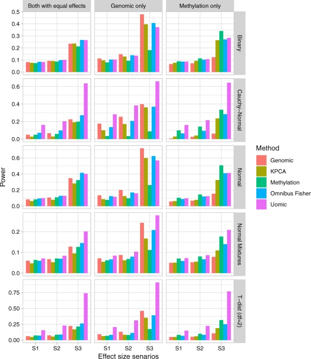
Power under different distributions of the outcomes (N = 500 and $\rho =0.1$). Effect size scenarios: S1: $G+M=0.04$ for normal and $G+M=0.08$ for the other distributions. S2: $G+M=0.05$ for normal and $G+M=0.1$ for the other distributions. S3: $G+M=0.1$ for normal and $G+M=0.2$ for the other distributions. G denotes the genetic effects (i.e. β_s) and M denotes the methylation effects (i.e. β_m). G = 0 (M = 0) when there is no genetic (methylation) effects. G = M when both genetic and methylation have the same effects

3.1.3. Simulation III: the impact of disease models

In this set of simulations, we evaluated the impact of different disease models on the performance of our method. In particular, we are interested in comparing different weighting schemes as outlined in Section 2.4. It is straightforward to show that when only two layers of omics data are considered, the consensus scheme is equivalent to that of the average weighting. Therefore, to thoroughly evaluate our method we considered three layers of omics data in this set of simulations. Without loss of generality, we simulated gene expression, methylation and genetic data for gene RB1. We used the InterSIM software, which simulates multiple interrelated data types with realistic intra/inter-relationships based on the TCGA ovarian cancer study, to generate gene expression and methylation data (Chalise et al., 2016). Since InterSIM software does not simulate genomic data, to mimic the real human genome, genetic variants within the RB1 gene were simulated using HAPGEN2 with the linkage disequilibrium structure the same as the CEU samples from the HAPMAP project (Su et al., 2011).

Outcomes were simulated using Equation (11), where they were associated with (i) none of the omics data (i.e. $I_{\mathrm{e}}=I_{\mathrm{s}}=I_{\mathrm{m}}=0$); (ii) only one layer of omics data (i.e. $I_{\mathrm{e}}\ne 0,I_{\mathrm{s}}=I_{\mathrm{m}}=0$ or $I_{\mathrm{s}}\ne 0,I_{\mathrm{e}}=I_{\mathrm{m}}=0$ or $I_{\mathrm{m}}\ne 0,I_{\mathrm{s}}=I_{\mathrm{e}}=0$); (iii) two layers of omics data (i.e. $I_{\mathrm{e}}\ne 0,I_{\mathrm{s}}\ne 0,I_{\mathrm{m}}=0$ or $I_{\mathrm{e}}\ne 0,I_{\mathrm{m}}\ne 0,I_{\mathrm{s}}=0$ or $I_{\mathrm{m}}\ne 0,I_{\mathrm{s}}\ne 0,I_{\mathrm{e}}=0$) and (iv) all omics data (i.e. $I_{\mathrm{m}}\ne 0,I_{\mathrm{s}}\ne 0,I_{\mathrm{e}}\ne 0$). Similar to the above simulations, X₁ and X₂ were continuous and binary covariates. J₁ and J₂ were the causal sets for genetic and methylation data, respectively. For the random errors, we considered two scenarios: (i) ${ϵ}_i\sim N(0,{\sigma }^2)$ and (ii) ${ϵ}_i\sim t_{\text{df}=2}$. The details of effect sizes for each scenario are in Supplementary Table S3. For our method, we considered four ways of constructing the ${\kappa }_{i,j}$: (i) the consensus weighting scheme as outlined in Section 2.4.1; (ii) the permutation-based weighting scheme as outlined in Section 2.4.2; (iii) the average weights and (iv) the optimal weighting scheme in which only the disease-associated layers of omics data were included in the association analysis. As KPCA was designed for only two layers of omics-data (Zhao et al., 2018), we only compared our methods to the method that combines correlated P-values (i.e. the Omnibus Fisher) and KMR models that assess associations for each layer of omics data (denoted by Genomic, Methylation and Expression).

$$\begin{array}{cc}{y}_i=\hfill & X_{1i}\times {\beta }_1+X_{2i}\times {\beta }_2+I_{\mathrm{s}}{\beta }_{\mathrm{s}}{\displaystyle \sum _{j\in J_1}}{G}_{i,j}\hfill \\ \hfill & +I_{\mathrm{m}}{\beta }_{\mathrm{m}}{\displaystyle \sum _{j\in J_2}}{M}_{i,j}+I_{\mathrm{e}}{\beta }_{\mathrm{e}}{E}_i+{ϵ}_i.\hfill \end{array}$$ (11)

The type I errors (i.e. none of the omics is related to the outcomes) and the empirical power when N = 500 are summarized in Tables 3 and 4, respectively. The corresponding results for N = 1000 are summarized in Supplementary Tables S4 and S5. The type I errors are well controlled for all settings. For normally distributed outcomes, the consensus weighting scheme performs similar to the permutation-based weighting scheme for most of the settings. The empirical power for both proposed weighting schemes is higher than that of the average weighting scheme. Moreover, the performance for both proposed weighting schemes is only slightly lower than the case, where only the associated layers of omics data are used for association analysis (i.e. ‘Uomic Optimal’). With regards to KMR-based methods, when multiple layers of omics data are associated with the outcomes, jointly considering all layers of omics data (i.e. Omnibus Fisher) outperforms the methods where only one layer of omics data is considered. Comparing to KMR-based models, our methods have better performance under most of the simulation settings. For outcomes that follow t-distribution with two degrees of freedom, similar trends hold except our methods significantly outperform KMR-based models. This indicates that the two proposed weighting schemes have robust performance against various underlying disease models regardless of the outcome distributions. We consider this important, as in practice we do not know which layers of omics data are associated with the outcomes of interest in advance.

Table 3.

Type I errors under different weighting schemes (N = 500)

Significance level	Uomic permutation	Uomic average	Uomic consensus	Genomic	Methylation	Expression	Omnibus Fisher
Normal distribution
0.050	0.0462	0.0462	0.0494	0.0502	0.0511	0.0506	0.0516
0.010	0.0088	0.0086	0.0094	0.0088	0.0091	0.0094	0.0084
0.005	0.0050	0.0046	0.0046	0.0040	0.0043	0.0040	0.0034
0.001	0.0002	0.0010	0.0012	0.0006	0.0006	0.0008	0.0008
T-dist (df = 2)
0.050	0.0492	0.0504	0.0504	0.0480	0.0442	0.0472	0.0472
0.010	0.0114	0.0120	0.0098	0.0084	0.0088	0.0068	0.0110
0.005	0.0062	0.0064	0.0062	0.0056	0.0043	0.0032	0.0062
0.001	0.0010	0.0008	0.0016	0.0018	0.0008	0.0010	0.0012

Table 4.

Power under different weighting schemes (N = 500)

Disease model	Uomic optimal	Uomic permutation	Uomic average	Uomic consensus	Genomic	Methylation	Expression	Omnibus Fisher
Normal distribution
E	0.5832	0.4224	0.3464	0.2116	0.0524	0.0528	0.3008	0.4510
M	0.8272	0.7272	0.5904	0.7098	0.0490	0.5954	0.0242	0.4612
M+E	0.9108	0.8542	0.7832	0.8260	0.0554	0.5944	0.2858	0.7186
G	0.7908	0.7046	0.5430	0.7248	0.7866	0.0446	0.0260	0.6842
G+E	0.8754	0.8294	0.7496	0.8216	0.7690	0.0548	0.3014	0.8412
G+M	0.9602	0.9326	0.8920	0.9568	0.7812	0.5954	0.0236	0.8492
G+M+E	0.9780	0.9620	0.9426	0.9780	0.7634	0.5956	0.2824	0.9206
T-dist (df = 2)
E	0.3488	0.2294	0.1952	0.1158	0.0448	0.0472	0.0730	0.0896
M	0.6324	0.5222	0.3860	0.5146	0.0884	0.1530	0.0408	0.1326
M+E	0.7028	0.6166	0.5312	0.5952	0.1084	0.1586	0.0830	0.1968
G	0.5716	0.4738	0.3276	0.4996	0.2166	0.0652	0.0316	0.1692
G+E	0.6752	0.6020	0.5040	0.5994	0.2526	0.0878	0.0906	0.2556
G+M	0.8206	0.7610	0.6724	0.8126	0.2896	0.1894	0.0572	0.2904
G+M+E	0.8554	0.8110	0.7606	0.8554	0.2848	0.1864	0.0962	0.3368

3.2 The analysis of Alzheimer’s disease dataset

We analyzed the whole genome sequencing and gene expression data from ADNI using the proposed method with the consensus weighting scheme. ADNI, including ADNI 1, ADNI GO and ADNI 2, is a longitudinal study that can assess the effects of biomarkers at various molecular levels on Alzheimer’s disease (AD). DNA samples from study subjects in ADNI 2 were obtained and analyzed using Illumina’s non-CLIA whole genome sequencing (Saykin et al., 2010). The baseline RNA expression data were collected from subjects in ADNI 2 at baseline for newly recruited subjects and 1st ADNI 2 visit for ADNI 1 and ADNI GO continuing subjects. We wish to identify biomarkers that are associated with cognitive test scores, including the Mini-Mental State Examination (MMSE), the 13-items Alzheimer’s Disease Assessment Scale-Cognitive Subscale (ADAS13), the Montreal Cognitive Assessment (MOCA) and the Clinical Dementia Rating Sum of Boxes (CDRSB). The distributions of these four cognitive scores are shown in Supplementary Figure S1. We focused on baseline data, and the sample sizes for genomic, gene expression and cognitive test scores are summarized in Supplementary Table S6. For genetic data, we annotated the genetic variants based on GRch37 assembly, and excluded genes with more than 20% missing. We included a total of 15 656 genes that have both genetic and gene expression data. For all association analyses, we controlled the effects of age and gender.

The QQ-plots and the Manhattan plots for the association analyses of all the four cognitive scores using the Uomic method are shown in Figures 3 and 4, respectively. The P-values for the associations between APOE and all the four cognitive test scores are highly significant (i.e. $P<{10}^{-5}$). There is substantial amount of evidence suggesting that the presence of the apolipoprotein ${\epsilon }_4$ allele is associated with an increased risk of AD (Christensen et al., 2008; Ertekin-Taner, 2007; Greenwood et al., 2000; Hoffmann et al., 2015). The proportions of individuals carrying at least ${\epsilon }_4$ allele among patients diagnosed with Alzheimer’s type dementia is much higher than those in the general population (Ertekin-Taner, 2007). Recent evidence also suggests that cognitive decline is more rapid for ${\epsilon }_4$ carriers as compared to the non-carries in the general population (Greenwood et al., 2000).

Fig. 3.

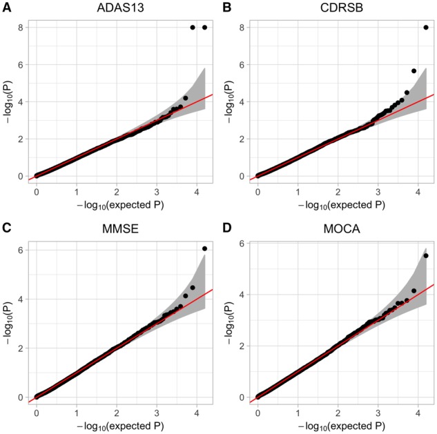
QQ-plots for association analyses of four cognitive test scores

Fig. 4.

Manhattan plots for association analyses of four cognitive test scores

For the ADAS13 and the Clinical Dementia Rating Scale, genes APOC1 and TOMM40 are also significant. A deletion/insertion polymorphism in the promoter region of the apolipoprotein C1 gene was reported to be associated with late-onset AD. APOC1 is a genetic risk factor for dementia and cognitive impairment in the elderly, and it has robust impact on hippocampal volumes (Serra-Grabulosa et al., 2003). It was also found that APOE ${\epsilon }_4$ carries with APOC1 insertion allele were much more prevalent among AD patients than healthy individuals (Zhou et al., 2014). For the gene TOMM40, the association between genetic variants within the TOMM40-APOE-${\epsilon }_4$-C1 region and the risk of AD has been established by a number of studies (Burggren et al., 2017; Chiba-Falek et al., 2018; Chu et al., 2011; Corder et al., 1993; Johnson et al., 2011; Maruszak et al., 2012). While some studies suggest that the association of TOMM40 poly-T, a polymorphism in intron 6 of the TOMM40 gene, is mainly due to its linkage disequilibrium with APOE (Chu et al., 2011; Corder et al., 1993; Maruszak et al., 2012). Others have supported the hypothesis of an independent association of TOMM40 poly-T with AD-related phenotypes [e.g. hippocampal thinning (Burggren et al., 2017) and gray matter volume (Johnson et al., 2011)]. Falek et al. found that TOMM40 poly-T was associated with changes in MOCA scores in the Bryan ADRC Prevention Screening Study and Database/Repository while adjusting for the effects of gender, age and APOE genotypes (Chiba-Falek et al., 2018). For the Clinical Dementia Rating Scale scores, the effect of TLR1 is also significant. It was found that TLR1 is up-regulated after AD onset (Hu, 2011). While TLR2 is a major receptor for Alzheimer’s amyloid β peptide that triggers neuroinflammatory activation, studies have suggested that TLR1 coexpression can enhance TLR-mediated $A\beta 42$-triggered inflammatory activation (Liu et al., 2012).

For the MMSE scores, in addition to gene APOE and APOC1, the gene SULF2 tends to be significant (i.e. $P=3.4\times {10}^{-5}$). Gene SULF2 modulates cell signaling, growth, development and homeostasis. Based on autopsy specimens from subjects with and without AD, it was found that the expression of SULF2 in AD patients was much lower in the hippocampal region, the parahippocampal gray matter and the frontal lobe gray matter. However, it is still not clear whether SULF2 is involved in the pathogenesis of AD, and further studies are needed to investigate the mechanisms for loss of SULF2 expression in AD living patients (Roberts et al., 2017).

For MOCA scores, in addition to APOE, gene SLC6A15 also tends to be significant (i.e. $P=7.1\times {10}^{-5}$). SLC6A15 gene, which belongs to the solute carrier family 6 (SLC6) and encodes a sodium-dependent transporter for neutral amino acids, was first shown to have effects on structural integrity of white matter tracts in major depressive disorder (Choi et al., 2016), and it is a regulator of hippocampal neurochemistry and behavior (Santarelli et al., 2015). While a recent study suggests SLC6A15 may be actively involved in AD (Ni et al., 2018), further studies are needed to investigate the role of SLC6A15 gene on the pathology of AD.

We also conducted the association analyses using the other three methods (i.e. Omnibus Fisher, KPCA and single-layer data analysis), and the QQ-plots and Manhattan plots are shown in Supplementary Figures S6 and S7, respectively. While the identified genes are largely consistent among all four methods (Supplementary Fig. S6), the type I errors for some outcomes can be inflated/conservative (Supplementary Fig. S6).

4 Discussion

We have proposed a flexible U-statistics-based non-parametric framework that comes with two weighting schemes for association analysis on multilayer omics data. There are three major advantages of our method. First, it can account for various levels of intercorrelations among multilayer omics data, as demonstrated through simulation studies (Fig. 1 and Supplementary Fig. S2), our method achieves better or similar power as compared to existing methods [i.e. KPCA (Zhao et al., 2018) and Omnibus Fisher (Yan et al., 2019)] at different levels of intercorrelations. Second, our method is built within the non-parametric U-statistics framework, and thus achieves robust and powerful performance for analyzing outcomes with various types of distributions (e.g. Gaussian, binary and heavy-tailed distributions). It can significantly outperform KMR-based methods when the distributions of outcomes are heavy tailed (Fig. 2 and Supplementary Figs S3–S5). Finally, our method can account for different possible disease models and obtain close to optimal power without entirely relying on resampling techniques. Indeed, while the permutation-based weighting scheme relies on resampling, the consensus weighting scheme can derive the P-value analytically. As shown in Table 4 and Supplementary Table S5, the consensus weighting scheme can achieve similar performance to that of the permutation-based scheme, and both schemes have better performance than KMR-based methods.

We used our method to test the association between omics data (i.e. gene expression and genetic variants) and four cognitive test scores obtained from ADNI study (Saykin et al., 2010). We have not only identified genes that are well known to be associated with AD (i.e. APOE, APOC1 and TOMM40), but also genes that have conflicted results (i.e. SLC6A15, SULF2 and TLR1). While our analyses have shed lights on the additional genes that may be associated with AD, further investigations are needed to study their pathology in AD development. While the association analysis of KMR-based method has slightly inflated type I errors for the Clinical Dementia Rating Scale scores and conservative P-values for the MOCA scores (Supplementary Fig. S6), there is no evidence of systematical inflation/deflation of our association results (Fig. 3).

Our proposed method has close connections with KMR-based methods, as all of them are in a quadratic form of kernel functions. While we focused on the main effects from each layer of omics data in this paper, it is straightforward to extend our method to consider interaction effects both within and across layers of omics data. For example, to consider pairwise interaction effects among genetic variants, a Hadamard product of a linear kernel that is constructed from genetic variants can be used to capture this pairwise interaction. Similarly, to consider interactions between genetic and methylation data, a Hadamard product between a linear kernel constructed from genetic data and another determined from methylation data can be used. Other kernel functions [e.g. saturate pathway kernel (Weissbrod et al., 2016)] can be used to capture more complex relationships. To assess the overall significance of all layers of omics data and their potential interaction effects, the same weighting schemes outlined in Section 2.4 can be used to obtain optimum power.

To adjust for the potential confounder effects, we project the outcomes to a subspace that is orthogonal to the space spanned by covariates, and rank the outcomes in this orthogonal subspace. While this approach is the same as ranking the residuals from a simple linear regression model, it may subject to suboptimal performance when the outcomes are binary or categorical, where residuals from generalized linear model are more appropriate. This is the future revenue of our research. Nevertheless, our proposed method has similar or better performance than the existing KMR-based methods regardless of the distributions of the outcomes.

References

- Ashley E.A. (2015) The precision medicine initiative: a new national effort. JAMA, 313, 2119–2120. [DOI] [PubMed] [Google Scholar]
- Bersanelli M. et al. (2016) Methods for the integration of multi-omics data: mathematical aspects. BMC Bioinformatics, 17 (Suppl. 2), 15. [DOI] [PMC free article] [PubMed] [Google Scholar]
- Burggren A.C. et al. (2017) Hippocampal thinning linked to longer TOMM40 poly-t variant lengths in the absence of the APOE epsilon4 variant. Alzheimers Dement., 13, 739–748. [DOI] [PMC free article] [PubMed] [Google Scholar]
- Chalise P. et al. (2016) InterSIM: simulation tool for multiple integrative ‘omic datasets’. Comput. Methods Programs Biomed., 128, 69–74. [DOI] [PMC free article] [PubMed] [Google Scholar]
- Chiba-Falek O. et al. (2018) The effects of the TOMM40 poly-t alleles on Alzheimer’s disease phenotypes. Alzheimers Dement., 14, 692–698. [DOI] [PMC free article] [PubMed] [Google Scholar]
- Choi S. et al. (2016) Effects of a polymorphism of the neuronal amino acid transporter SLC6A15 gene on structural integrity of white matter tracts in major depressive disorder. PLoS One, 11, e0164301. [DOI] [PMC free article] [PubMed] [Google Scholar]
- Christensen H. et al. (2008) The association of APOE genotype and cognitive decline in interaction with risk factors in a 65–69 year old community sample. BMC Geriatr., 8, 14. [DOI] [PMC free article] [PubMed] [Google Scholar]
- Chu S.H. et al. (2011) TOMM40 poly-t repeat lengths, age of onset and psychosis risk in Alzheimer’s disease. Neurobiol. Aging, 32, 2328.e1–2328.e9. [DOI] [PMC free article] [PubMed] [Google Scholar]
- Corder E.H. et al. (1993) Gene dose of apolipoprotein E type 4 allele and the risk of Alzheimer’s disease in late onset families. Science, 261, 921–923. [DOI] [PubMed] [Google Scholar]
- do Valle I.F. et al. (2018) Network integration of multi-tumour omics data suggests novel targeting strategies. Nat. Commun., 9, 4514. [DOI] [PMC free article] [PubMed] [Google Scholar]
- Ertekin-Taner N. (2007) Genetics of Alzheimer’s disease: a centennial review. Neurol. Clin., 25, 611–667, v. [DOI] [PMC free article] [PubMed] [Google Scholar]
- Greenwood P.M. et al. (2000) Genetics and visual attention: selective deficits in healthy adult carriers of the epsilon4 allele of the apolipoprotein E gene. Proc. Natl. Acad. Sci. USA, 97, 11661–11666. [DOI] [PMC free article] [PubMed] [Google Scholar]
- Hoeffding W. (1948) A class of statistics with asymptotically normal distribution. Ann. Math. Stat., 19, 293–325. [Google Scholar]
- Hoffmann K. et al. (2015) Moderate-to-high intensity physical exercise in patients with Alzheimer’s disease: a randomized controlled trial. J. Alzheimers Dis., 50, 443–453. [DOI] [PubMed] [Google Scholar]
- Hu W. (2011) Alzheimer’s disease is TH17 related autoimmune disease against misfolded beta amyloid. Nat. Precedings, doi: 10.1038/npre.2011.5934.3. [Google Scholar]
- Huang Y.T. (2014) Integrative modeling of multiple genomic data from different types of genetic association studies. Biostatistics, 15, 587–602. [DOI] [PubMed] [Google Scholar]
- Huang Y.T. et al. (2014) Joint analysis of SNP and gene expression data in genetic association studies of complex diseases. Ann. Appl. Stat., 8, 352–376. [DOI] [PMC free article] [PubMed] [Google Scholar]
- Johnson S.C. et al. (2011) The effect of TOMM40 poly-t length on gray matter volume and cognition in middle-aged persons with APOE epsilon3/epsilon3 genotype. Alzheimers Dement., 7, 456–465. [DOI] [PMC free article] [PubMed] [Google Scholar]
- Lee S. et al. (2012) Optimal tests for rare variant effects in sequencing association studies. Biostatistics, 13, 762–775. [DOI] [PMC free article] [PubMed] [Google Scholar]
- Li Y. et al. (2018) A review on machine learning principles for multi-view biological data integration. Brief. Bioinform., 19, 325–340. [DOI] [PubMed] [Google Scholar]
- Liu S. et al. (2012) TLR2 is a primary receptor for Alzheimer’s amyloid beta peptide to trigger neuroinflammatory activation. J. Immunol., 188, 1098–1107. [DOI] [PubMed] [Google Scholar]
- Manolio T.A. et al. (2009) Finding the missing heritability of complex diseases. Nature, 461, 747–753. [DOI] [PMC free article] [PubMed] [Google Scholar]
- Mariette J., Villa-Vialaneix N. (2018) Unsupervised multiple kernel learning for heterogeneous data integration. Bioinformatics, 34, 1009–1015. [DOI] [PubMed] [Google Scholar]
- Maruszak A. et al. (2012) TOMM40 rs10524523 polymorphism’s role in late-onset Alzheimer’s disease and in longevity. J. Alzheimers Dis., 28, 309–322. [DOI] [PubMed] [Google Scholar]
- Ni H. et al. (2018) The GWAS risk genes for depression may be actively involved in Alzheimer’s disease. J. Alzheimers Dis., 64, 1149–1161. [DOI] [PubMed] [Google Scholar]
- Phan J.H. et al. (2012) Multiscale integration of -omic, imaging, and clinical data in biomedical informatics. IEEE Rev. Biomed. Eng., 5, 74–87. [DOI] [PMC free article] [PubMed] [Google Scholar]
- Poole W. et al. (2016) Combining dependent P-values with an empirical adaptation of Brown’s method. Bioinformatics, 32, i430–436. [DOI] [PMC free article] [PubMed] [Google Scholar]
- Roberts R.O. et al. (2017) Decreased expression of Sulfatase 2 in the brains of Alzheimer’s disease patients: implications for regulation of neuronal cell signaling. J. Alzheimers Dis. Rep., 1, 115–124. [DOI] [PMC free article] [PubMed] [Google Scholar]
- Santarelli S. et al. (2015) The amino acid transporter SLC6A15 is a regulator of hippocampal neurochemistry and behavior. J. Psychiatr. Res., 68, 261–269. [DOI] [PubMed] [Google Scholar]
- Saykin A.J. et al. (2010) Alzheimer’s Disease Neuroimaging Initiative biomarkers as quantitative phenotypes: genetics core aims, progress, and plans. Alzheimers Dement., 6, 265–273. [DOI] [PMC free article] [PubMed] [Google Scholar]
- Serra-Grabulosa J.M. et al. (2003) Apolipoproteins E and C1 and brain morphology in memory impaired elders. Neurogenetics, 4, 141–146. [DOI] [PubMed] [Google Scholar]
- Shieh G.S. (1997) Weighted degenerate U- and V-statistics with estimated parameters. Stat. Sin., 7, 1021–1038. [Google Scholar]
- Su Z. et al. (2011) HAPGEN2: simulation of multiple disease SNPs. Bioinformatics, 27, 2304–2305. [DOI] [PMC free article] [PubMed] [Google Scholar]
- Wei C. et al. (2016) A weighted U statistic for association analyses considering genetic heterogeneity. Stat. Med., 35, 2802–2814. [DOI] [PMC free article] [PubMed] [Google Scholar]
- Weissbrod O. et al. (2016) Multikernel linear mixed models for complex phenotype prediction. Genome Res., 26, 969–979. [DOI] [PMC free article] [PubMed] [Google Scholar]
- Wu C., Ma S. (2015) A selective review of robust variable selection with applications in bioinformatics. Brief. Bioinform., 16, 873–883. [DOI] [PMC free article] [PubMed] [Google Scholar]
- Wu C. et al. (2019) A Selective Review of Multi-Level Omics Data Integration Using Variable Selection. High-Throughput, 8, 4. [DOI] [PMC free article] [PubMed] [Google Scholar]
- Wu M.C. et al. (2010) Powerful SNP-set analysis for case–control genome-wide association studies. Am. J. Hum. Genet., 86, 929–942. [DOI] [PMC free article] [PubMed] [Google Scholar]
- Wu M.C. et al. (2011) Rare-variant association testing for sequencing data with the sequence kernel association test. Am. J. Hum. Genet., 89, 82–93. [DOI] [PMC free article] [PubMed] [Google Scholar]
- Yan Q. et al. (2019) An integrative association method for omics data based on a modified fisher’s method with application to childhood asthma. PLoS Genet., 15, e1008142. [DOI] [PMC free article] [PubMed] [Google Scholar]
- Zeng I.S.L., Lumley T. (2018) Review of statistical learning methods in integrated omics studies (an integrated information science). Bioinform. Biol. Insights, 12, 117793221875929. [DOI] [PMC free article] [PubMed] [Google Scholar]
- Zhao N. et al. (2018) Kernel machine methods for integrative analysis of genome-wide methylation and genotyping studies. Genet Epidemiol., 42, 156–167. [DOI] [PubMed] [Google Scholar]
- Zhao S.D. et al. (2014) More powerful genetic association testing via a new statistical framework for integrative genomics. Biometrics, 70, 881–890. [DOI] [PMC free article] [PubMed] [Google Scholar]
- Zhou Q. et al. (2014) Association between APOC1 polymorphism and Alzheimer’s disease: a case–control study and meta-analysis. PLoS One, 9, e87017. [DOI] [PMC free article] [PubMed] [Google Scholar]
Associated Data
This section collects any data citations, data availability statements, or supplementary materials included in this article.