Abstract
Deep neural networks can directly learn from chemical structures without extensive, user-driven selection of descriptors in order to predict molecular properties/activities with high reliability. But these approaches typically require large training sets to learn the endpoint-specific structural features and ensure reasonable prediction accuracy. Even though large datasets are becoming the new normal in drug discovery, especially when it comes to high-throughput screening or metabolomics datasets, one should also consider smaller datasets with challenging endpoints to model and forecast. Thus, it would be highly relevant to better utilize the tremendous compendium of unlabeled compounds from publicly-available datasets for improving the model performances for the user’s particular series of compounds. In this study, we propose the Molecular Prediction Model Fine-Tuning (MolPMoFiT) approach, an effective transfer learning method based on self-supervised pre-training + task-specific fine-tuning for QSPR/QSAR modeling. A large-scale molecular structure prediction model is pre-trained using one million unlabeled molecules from ChEMBL in a self-supervised learning manner, and can then be fine-tuned on various QSPR/QSAR tasks for smaller chemical datasets with specific endpoints. Herein, the method is evaluated on four benchmark datasets (lipophilicity, FreeSolv, HIV, and blood–brain barrier penetration). The results showed the method can achieve strong performances for all four datasets compared to other state-of-the-art machine learning modeling techniques reported in the literature so far.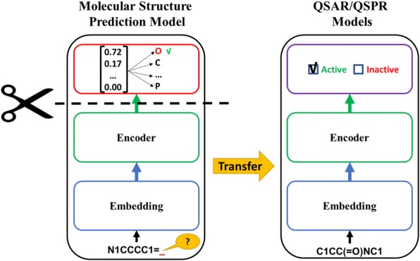
Keywords: Transfer learning, Neural networks, Self-supervised learning, QSPR/QSAR
Introduction
Predicting properties/activities of chemicals from their structures is one of the key objectives in cheminformatics and molecular modeling. Quantitative structure property/activity relationship (QSPR/QSAR) modeling [1–6] relies on machine learning techniques to establish quantified links between molecular structures and their experimental properties/activities. When using a classic machine learning approach, the training process is divided into two main steps: feature extraction/calculation and the actual modeling. The features (also called descriptors) characterizing the molecular structures are critical for the model performances. They typically encompass 2D molecular fingerprints, topological indices, or substructural fragments, as well as more complex 3D and 4D descriptors [7, 8] directly computed from the molecular structures [9].
Deep learning methods have demonstrated remarkable performances in several QSPR/QSAR case studies. In addition to use expert-engineered molecular descriptors as input, those techniques can also directly take molecular structures (e.g., molecular graph [10–21], SMILES strings [22–24], and molecular 2D/3D grid image [25–30]) and learn the data-driven feature representations for predicting properties/activities. As a result, this type of approach is potentially able to capture and extract underlying, complex structural patterns and feature ↔ property relationships given sufficient amount of training data. The knowledge derived from these dataset-specific descriptors can then be used to better interpret and understand the structure–property relationships as well as to design new compounds. In a large scale benchmark study, Yang et al. [12] shown that a graph convolutional model that construct a learned representation from molecular graph consistently matches or outperforms models trained with expert-engineered molecular descriptors/fingerprints.
Graph convolutional neural networks (GCNN) directly operate on molecular graphs [10]. A molecular graph is an undirected graph whose nodes correspond to the atoms of the molecule and edges correspond to chemical bonds. GCNNs iteratively update the nodes representation by aggregating the representations of their neighboring nodes and/or edges. After k iterations of aggregation, the final nodes representations capture the local structure information within their k-hop graph neighborhood (which is somehow similar to augmented substructural fragments [31] but in a more data-driven manner). Moreover, the Simplified Molecular-Input Line-Entry System (SMILES) [32, 33] encodes the molecular structures as strings of text. Widely used in the field of cheminformatics, the SMILES format can be considered as an analogue of natural language. As a result, deep learning model architectures such as RNNs [34, 35], CNNs [36] and transformers [37] can be directly applied to SMILES for QSAR/QSPR tasks. While deep learning models have achieved state-of-the-art results on a variety of molecular properties/activities prediction tasks, these end-to-end models require very large amount of training data to learn useful feature representations. The learned representations are usually endpoint-specific, which means the models need to be built and retrained from scratch for the new endpoint/dataset of interest. Small chemical datasets with challenging endpoints to model are thus still disadvantaged with these techniques and unlikely to lead to models with reasonable prediction accuracy. As of today, this is considered as a grand challenge for QSAR modelers facing small sets of compounds without a clear path for obtaining reliable models for the endpoint of interest.
Meanwhile, transfer learning is a quickly emerging technique based on the general idea of reusing a pre-trained model built on a large dataset as the starting point for building a new, more optimized model for a target endpoint of interest. It is now widely used in the field of computer vision (CV) and natural language processing (NLP). In CV, a pre-trained deep learning model on ImageNet [38] can be used as the start point to fine-tune for a new task [39]. Transfer learning in NLP has historically been restricted to the shallow word embeddings: NLP models start with embedding layers initialized with pretrained weights from Word2Vec [40], GloVe [41] or fastText [42]. This approach only uses the prior knowledge for the first layer of a model, the remaining layers still need to be trained and optimized from scratch. Language model pre-training [43–47] extends this approach by transferring all the learned optimized weights from multiple layers, which providing contextualized word embeddings for the downstream tasks. Language scale pre-trained language models have greatly improved the performance on a variety of language tasks. The default task for a language model is to predict the next word given the past sequence. The input and labels of the dataset used to train a language model are provided by the text itself. This is known as self-supervised learning. Self-supervised learning opens up a huge opportunity for better utilizing unlabeled data.
Due to the limited amount and sparsity of labeled datasets for certain types of endpoints in chemistry (e.g., inhibitor residence times, allosteric inhibition, renal clearance), several transfer learning methods have been developed for allowing the development of QSPR/QSAR models for those types of endpoints/datasets. Inspired by ImageNet pretraining, Goh et al. proposed ChemNet [26] for transferable chemical property prediction. A deep neural network was pre-trained in a supervised manner on the ChEMBL [48] database using computed molecular descriptors as labels, then fine-tuned on other QSPR/QSAR tasks. Jaeger et al. [49] developed Mol2vec which employed the same idea of Word2Vec in NLP. Mol2vec learns the vector representations of molecular substructures in an unsupervised learning manner. Vectors of closely related molecular substructures are close to each other in the vector space. Molecular representations are computed by summing up the vectors of the individual substructures and be used as input for QSPR/QSAR models. Hu et al. pre-trained graph neural networks (GNNs) using both unlabeled data and labeled data from related auxiliary supervised tasks. The pre-trained GNNs were shown to significantly increase the model performances [50]. Multitask learning (MLT) is a related field to transfer learning, aiming at improving the performance of multiple tasks by learning them jointly. Multitask DNNs (deep neural networks) for QSAR were notably introduced by the winning team in the Kaggle QSAR competition and then applied in other QSAR/QSPR studies [51–56]. MTL is particularly useful if the endpoints share a significant relationship. However, MTL requires the tasks to be trained from scratch every time.
Herein, we propose the Molecular Prediction Model Fine-Tuning (MolPMoFiT − pronounced MOLMOFIT), an effective transfer learning method based on self-supervised pre-training + task-specific fine-tuning for QSPR/QSAR modeling. In the current version, a molecular structure prediction model (MSPM) is pre-trained using one million bioactive molecules from ChEMBL and then fine-tuned for various QSPR/QSAR tasks. This method is “universal” in the sense that the pre-trained molecular structure prediction model can be used as a source for any other QSPR/QSAR models dedicated to a specific endpoint and a smaller dataset (e.g., molecular series of congeneric compounds). This approach could constitute a first look at next-gen QSAR models being capable of high prediction reliability even for small series of compounds and highly challenging endpoints.
Methods
ULMFiT
The MolPMoFiT method we proposed here is adapted from the ULMFiT (Universal Language Model Fine-Tuning) [45], a transfer learning method developed for any NLP classification tasks. The original implementation of ULMFiT breaks the training process into three stages:
Train a general domain language model in the self-supervised manner on a large corpus (e.g., Wikitext-103 [57]). Language models are a type of model that aim to predict the next word in the sentences given the context precede it. The input and labels of the dataset used to train a language model are provided by the text itself. After training on millions of unlabeled text, the language model captures the extensive and in-depth knowledge [58–60] of a language and can provide useful features for other NLP tasks.
Fine-tuning the general language model on the task corpus to create a task specific language model.
Fine-tuning the task specific language model for downstream classification/regression model.
As described above, the ULMFiT is a three-stage transfer learning process that includes two types of models: language models and classification/regression models. A language model is a model that takes in a sequence of words and predicts the most likely next word. A language model is trained in a self-supervised manner and no label is required. This means the training data can be generated from a huge amount of unlabeled text data. The classification/regression model is a model that takes a whole sequence and predicts the class/value associated to the sequence, requiring labeled data.
MolPMoFiT
In this study, we adapted the ULMFiT method to handle molecular property/activity prediction. Specifically, we trained a molecular structure prediction model (MSPM) using one million molecules extracted from ChEMBL with self-supervised learning. The pre-trained MSPM was then fine-tuned for the given QSAR/QSPR tasks.
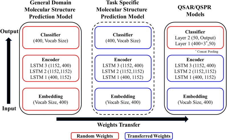
Model Architecture: The architectures for the MSPMs and the QSAR/QSPR models follow similar structures (Fig. 1): the embedding layer, the encoder and the classifier. The embedding layer converts the numericized tokens into fixed length vector representations (see “Molecular representation” section for details); the encoder processes the sequence of embedding vectors into feature representations which contain the contextualized token meanings; and the classifier uses the extracted feature representations to make the final prediction. The model architecture used for modeling is AWD-LSTM (ASGD Weight-Dropped LSTM) [61]. The main idea of the AWD-LSTM is to use a LSTM (Long Short-Term Memory [62]) model with dropouts in all the possible layers (embedding layer, input layer, weights, and hidden layers). The model hyperparameters are same as the ones initially implemented for ULMFiT. An embedding vector length of 400 was used for the models. The encoder consisted of three LSTM layers: the input size of first LSTM layer is 400, the hidden number of hidden units is 1152, and the output size of the last LSTM layer is 400. The classifiers use the output of the encoder to make predictions. The MSPMs and QSPR/QSAR models use the output of the encoder in different ways for different prediction purposes. The MSPM classifier consists of just a single softmax layer. The MSPMs predict the next token in a SMILES string, using the hidden state at the last time step hT of the final LSTM layer of the encoder. The QSPR/QSAR model classifier consists of two feedforward neural network layers. The first layer takes the concatenation of output vectors from the last LSTM layer of the encoder (concatenation of max pooling, mean pooling and last time step hT [45]), followed by a ReLU activation function. The final output size is determined by the QSPR/QSAR endpoints, e.g., for regression models, a single output node is used; for classification models, the output size equals to the number of classes.
Fig. 1.
Scheme illustrating the MolPMoFiT Architecture: During the fine-tuning, learned weights are transferred between models. Vocab Size corresponds to the number of unique characters tokenized (see “Molecular representation” section) from SMILES in a data set. The stage of Task Specific Molecular Structure Prediction Model fine-tuning is optional
General-Domain MSPM Training: In the first stage of training, a general domain MSPM is trained on one million molecules curated from ChEMBL. The model is trained using the one cycle policy with a constant learning rate for 10 epochs. One cycle policy is a learning rate schedule method proposed by Smith [63]. The MSPM forms the source for all the subsequent QSPR/QSAR models. The training of the general-domain MSPM model requires about one day on a single NVIDIA Quadro P4000 GPU but it only needs to be trained once and can be reused for other QSPR/QSAR tasks.
Task Specific MSPM Model Fine-Tuning (Optional): The stage is optional for MolPMoFiT. The MSPM trained on ChEMBL covers a large and diverse chemical space of bioactive molecules and can be directly fine-tuned to predict physical properties of molecules such as lipophilicity and solubility. For bioactivities such as HIV inhibition and other drug activities, scientists are more interested in compounds with desired activities. The experimental tested data (target task dataset) may have a different distribution from ChEMBL. Fine-tuning the general domain MSPM on target task data to adapt to the idiosyncrasies of the task data would be helpful to the downstream QSAR models. The impact of task specific MSPM fine-tuning will be analyzed in “Benchmark” section.
In this stage, the goal is to fine-tuning the general domain MSPM on the target QSAR datasets to create the task-specific (endpoint-specific) MSPM. The initial weights (embedding, encoder and linear head) of task specific MSPM are transferred from the general domain MSPM. The task specific MSPMs are fine-tuned using the one cycle policy and discriminative fine-tuning [45]. In a neural network, different layers encode different levels of information [64]. Higher layers contain less general knowledge toward the target task and need more fine-tuning compared to lower layers. Instead of using the same learning rate for fine-tuning all the layers, the discriminative fine-tuning trains higher layers with higher learning rates. Learning rates are adjusted based on the same the function ηlayer − 1 = ηlayer/2.6 used in the original ULMFiT approach, where η is the learning rate.
QSAR/QSPR Models Fine-Tuning: When fine-tuning the QSAR/QSPR model, only the embedding layer and the encoder are transferred from the pre-trained model, as the QSAR/QSPR model required a different classifier. In other word, the weights of classifier are initialized randomly and need to be trained from scratch for each task [45]. The QSPR/QSAR model is fine-tuned using one cycle policy, discriminative fine-tuning and gradual unfreezing [45]. During the fine-tuning, the model is gradually unfrozen over four layer-groups: (i) classifier; (ii) classifier + final LSTM layer; (iii) classifier + final two LSTM layers, and (iv) full model. Gradual unfreezing first trains the classifier of the model with the embedding and encoder layers frozen (weights are not updated). Then unfreezing the second to last layer-groups and fine-tuning the model. This process continues until all the layer-groups are unfrozen and fine-tuned.
Implementation. We implemented our model using the PyTorch [65] (https://pytorch.org/) deep learning framework and fastai v1 library [66] (https://docs.fast.ai). To ensure the reproducibility of this study, the data and code used in this study are freely available at: https://github.com/XinhaoLi74/MolPMoFiT.
Dataset preparation
SMILES of all molecules in ChEMBL [48] were downloaded and curated following the procedure: (1) Removing mixtures, molecules with more than 50 heavy atoms (2) Standardizing with MolVS [67] package; (3) Sanitizing and canonizing with RDKit [68] package. After curation, one million SMILES were randomly selected for training and testing the molecular structure perdition model.
We tested our method on four publicly-available, benchmark datasets [15]: (1) molecular lipophilicity; (2) experimental measured solvation energy in kcal/mol (FreeSolv) (3) HIV inhibition, and (4) blood–brain barrier penetration (BBBP). The detailed descriptions are summarized in Table 1.
Table 1.
Description of QSAR/QSPR datasets
| Data Set | Description | Size | # of active compound | Task |
|---|---|---|---|---|
| Lipophilicity | Octanol/water distribution coefficient | 4200 | Regression | |
| FreeSolv | Experimental measured solvation energy (kcal/mol) | 642 | Regression | |
| HIV | Inhibition of HIV replication | 41,127 | 1443 | Classification |
| BBBP | Ability to penetrate the blood–brain barrier | 2039 | 1560 | Classification |
Molecular representation
In this study, we use SMILES strings as the textual representation of molecules. SMILES is a linear notation for representing molecular structures. For SMILES to be processed by machine learning models, they need to be transformed into numeric representations. SMILES strings are tokenized at the character level with a few specific treatments: (1) ‘Cl’, ‘Br’ are two-character tokens; (2) special characters encoded between brackets are considered as tokens (e.g., ‘[nH], ‘[O-]’ and ‘[Te]’ et al.). The unique tokens are mapped to integers to be used as input for the deep learning models.
Data Augmentation
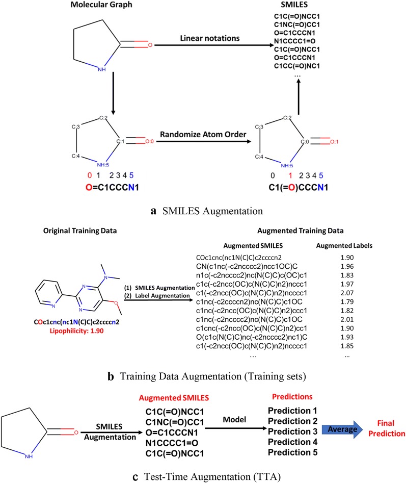
Deep learning models are data-hungry so that various data augmentation techniques have been developed for different types of data and applications [69–72]. Data augmentation usually helps deep learning models to be better generalized for new data. Each SMILES corresponds to one unique molecular structure, whereas several SMILES strings can be derived from the same molecule. In fact, for a single molecular structure, many SMILES can be generated by simply randomizing the atom ordering (Fig. 2a). Bjerrum shown the SMILES enumeration as a data augmentation technique for QSAR models based on SMILES input can improve the robustness and accuracy [73]. It has been also shown that the generative models trained on both augmented and canonical SMILES can create a larger chemical space of structures [74, 75]. Herein, we used SMILES enumeration as the basis for data augmentation technique. The SMILES augmentation technique was applied to both the MSPM and QSAR/QSPR models. For MSPM, the SMILES augmentation ensures the trained model can cover a large and diverse chemical space (characterized by SMILES). For unbalanced classification QSAR/QSPR datasets, the SMILES augmentation can be applied to re-balance the class distribution of training data. In addition to SMILES augmentation, for regression QSAR/QSPR models, a Gaussian noise (mean set at 0 and standard deviation σnoise) is added to the labels of augmented SMILES which could be considered as a simulation of experimental errors [76]. (Figure 2b). The standard deviation σnoise is considered as a hyperparameter for the models and need to be tuned from task to task. The impact of training data augmentation will be analyzed in “Analysis” section.
Fig. 2.
SMILES and Data Augmentation
We also applied the test time augmentation (TTA): Briefly, the final predictions are generated by averaging predictions of the canonical SMILES and four augmented SMILES (Fig. 2c). The impact of TTA will be discussed in “Benchmark” section.
Baselines and comparison models
To evaluate the performance of our method, we compared our models to the models reported by Yang et al. [12], including directed message passing neural network (D-MPNN), D-MPNN with RDKit features, random forest (RF) model on binary Morgan fingerprints, feed-forward network (FFN) on binary Morgan fingerprints, FFN on count-based Morgan fingerprints and FFN on RDKit descriptors,. We evaluated all models based on the original random and scaffold splits from Yang et al. for a fair and reproducible comparison. All the models were evaluated on the test sets on 10 randomly seeded 80:10:10 data splits. For regression model, we use root-mean-square-error (RMSE) as the key metric. For classification model, we use area under the receiver operating characteristic curve (AUROC) as the key metric.
Hyperparameters and Training Procedure
QSAR/QSPR Model Fine-Tuning: We are interested in obtaining a model that perform robustly across a variety of QSPR/QSAR tasks. Herein, we used the same set of hyperparameters for fine-tuning QSPR/QSAR models across different tasks, which we tuned on the HIV dataset (Table 2). The batch size is set to 128 (64 for HIV dataset due to the GPU memory limit). The optimal hyperparameters of the HIV dataset was determined based on the validation set results on 3 randomly 80:10:10 data splits. Specifically, we optimized the dropout rates, the base learning rate and training epochs.
Table 2.
Hyperparameters for QSPR/QSAR Model Fine-tuning
| Layer groups | Base Learning Rate | Epochs |
|---|---|---|
| Linear head only | 3e−2 | 4 |
| Linear head + final LSTM layer | 5e−3 | 4 |
| Linear head + final two LSTM layers | 5e−4 | 4 |
| Full model | 5e−5 | 6 |
Data Augmentation: In order to train a molecular structure prediction model that can be applied to a large chemical space, ChEMBL data is augmented by 4 times in addition to the original canonical SMILES. For the lipophilicity and FreeSolv datasets (regression), the number of augmented SMILES and the label noise σnoise were tuned on the validation set on three 80:10:10 random split. Specifically, the SMILES of lipophilicity training data were augmented 25 times with the label noise σnoise = 0.3 and the SMILES of FreeSolv training data were augmented 50 times with the label noise σnoise = 0.5. For classification tasks, we used data augmentation to balance the class distribution. Specifically, for HIV data, the SMILES of active class were augmented 60 times and the SMILES of inactive class were augmented 2 times. For BBBP data, the SMILES of positive class were augmented 10 times and the SMILES of negative class were augmented 30 times.
Results and discussion
Benchmark
Yang et al. [12] developed a graph convolutional model based on directed message passing neural network (D-MPNN) and benchmarked it across a wide variety of public and proprietary datasets, achieved consistently strong performance. We benchmarked our MolPMoFiT method to the state-of-the-art models from Yang et al. on four well-studied chemical datasets: lipophilicity, FreeSolv, HIV and BBBP. Both random and scaffold splits were evaluated. Scaffold split enforced all training and test sets shared no common molecular scaffolds, which represent a more challenging and realistic evaluation compared to a random split. All the models were evaluated on test set on the exact same ten 80:10:10 splits from Yang et al. to ensure a fair and reproducible benchmark. Results for lipophilicity and FreeSolv data were evaluated by root mean square error (RMSE), whereas results for HIV and BBBP were evaluated by area under the receiver operating characteristic curve (AUROC). For physical properties lipophilicity and FreeSolv data, the regression models were fine-tuned on the general domain MSPM. For bioactivities HIV and BBBP data, the classification models were fine-tuned on both the general and task-specific MSPMs (see “MolPMoFiT” section). Evaluation metrics were computed in two settings: (1) testing on canonical SMILES only and (2) Time-time augmentation (TTA, see “Data augmentation” section).
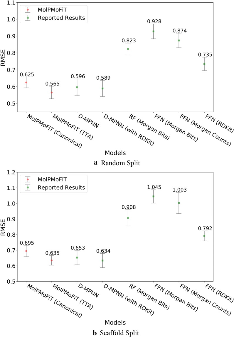
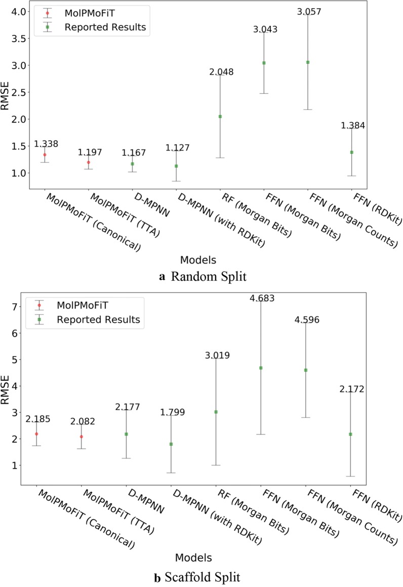
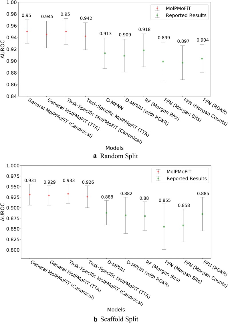
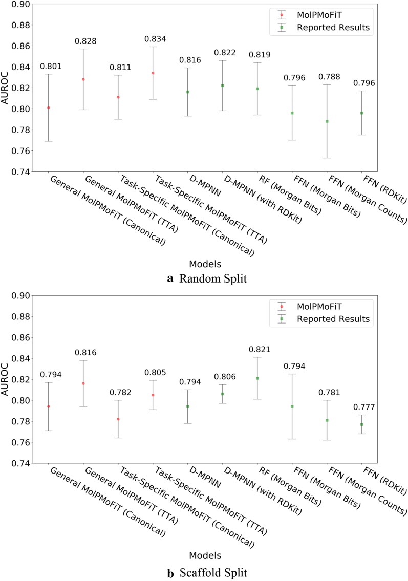
The results for test sets are summarized in Figs. 3, 4, 5 and 6. Across all four data sets, MolPMoFiT models achieved comparable or better prediction performances compared to the baselines. Generally, a scaffold split resulted in a worse performance compared to a random split. But a scaffold split can better measure the generalization ability of a model, which is very useful [77] for new molecular series with scaffolds being dissimilar to any other compounds in the modeling set.
Fig. 3.
Comparison of MolPMoFiT to Reported Results from Yang’s [12] on Lipophilicity. a Random split; b Scaffold split. MolPMoFiT Molecular Prediction Model Fine-Tuning, D-MPNN Directed Message Passing Neural Network, RF Random Forest, FFN Feed-Forward Network
Fig. 4.
Comparison of MolPMoFiT to Reported Results from Yang’s [12] on FreeSolv. a Random split; b Scaffold split
Fig. 5.
Comparison of MolPMoFiT to Reported Results from Yang’s [12] on BBBP. a Random split; b Scaffold split
Fig. 6.
Comparison of MolPMoFiT to Reported Results from Yang’s [12] on HIV. a Random split; b Scaffold split
For lipophilicity data, MolPMoFiT models tested on TTA outperform those tested on canonical SMILES. On random split, MolPMoFiT achieved a test set RMSE of 0.565 ± 0.037 and 0.625 ± 0.032 with and without TTA, respectively (Fig. 3a). On scaffold split, MolPMoFiT achieved a test set RMSE of 0.635 ± 0.031 and 0.695 ± 0.036 with and without TTA, respectively (Fig. 3b).
The FreeSolv dataset only contains 642 compounds, different data splits resulted in a large variance in RMSE (Fig. 4). MolPMoFiT models tested on TTA outperform those tested on canonical SMILES on random split but have no significant difference on scaffold split. On random split, MolPMoFiT achieved a test set RMSE of 1.197 ± 0.127 and 1.338 ± 0.144 with and without TTA, respectively (Fig. 4a). On scaffold split, MolPMoFiT achieved a test set RMSE of 2.082 ± 0.460 and 2.185 ± 0.448 with and without TTA, respectively (Fig. 4b).
For bioactivities like BBBP and HIV inhibition, the molecules of interest (tested experimentally) may have a different distribution from ChEMBL. Fine-tuning the general domain MSPM on target task data to adapt to the idiosyncrasies of the task data would be helpful to the downstream QSAR models. We evaluated the QSAR models fine-tuned both on general domain MSPM (named as general MolPMoFiT) and task-specific MSPM (named as task-specific MolPMoFiT) on BBBP and HIV datasets. For both BBBP (Fig. 5) and HIV (Fig. 6) dataset, the performance of models fine-tuned on general domain MSPM is on-par with the performance of models fine-tuned on the task-specific MSPMs. It requires more case studies to show whether fine-tuning on task-specific MSPM is beneficial.
On BBBP dataset, MolPMoFiT models outperform other comparison models (Fig. 5). Specifically, the general MolPMoFiT models achieved a test set AUROC of 0.950 ± 0.020 (Canonical SMILES) and 0.945 ± 0.023 (TTA) on random split and achieved a test set AUROC of 0.931 ± 0.025 (Canonical SMILES) and 0.929 ± 0.023 (TTA) on scaffold split. The task-specific MolPMoFiT models achieved a test set AUROC of 0.950 ± 0.022 (Canonical SMILES) and 0.942 ± 0.023 (TTA) on random split and achieved a test set AUROC of 0.933 ± 0.023 (Canonical SMILES) and 0.926 ± 0.026 (TTA) on scaffold split. It is worth noting that the implementation of TTA shows no improvements of the model accuracy.
For HIV data (Fig. 6), the general MolPMoFiT models achieved a test set AUROC of 0.801 ± 0.032 (Canonical SMILES) and 0.828 ± 0.029 (TTA) on random split and achieved a test set AUROC of 0.794 ± 0.023 (Canonical SMILES) and 0.816 ± 0.022 (TTA) on scaffold split. The task-specific MolPMoFiT models achieved a test set AUROC of 0.811 ± 0.021 (Canonical SMILES) and 0.834 ± 0.025 (TTA) on random split and achieved a test set AUROC of 0.782 ± 0.018 (Canonical SMILES) and 0.805 ± 0.014 (TTA) on scaffold split.
Analysis
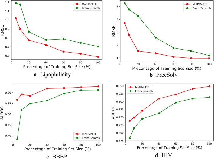
Impact of Transfer Learning: MolPMoFiT models were compared to the models that were trained from scratch. The models were trained on different number of training data and tested on the test set on a single 80:10:10 random split. The hyperparameters (learning rate, dropout rate and training epochs) were kept fixed: the hyperparameters of MolPMoFiT models were the same as we used in benchmark and the hyperparameters of models trained from scratch were tuned based on the validation set using the full training set. The results are illustrated in Fig. 7. Generally, with different numbers of training data, the MolPMoFiT model always outperforms the model trained from scratch. This indicated that the MolPMoFiT transfer learning technique provided a robust improvement for the model performances.
Fig. 7.
Performances of models on the different size of the training set. a Lipophilicity; b FreeSolv; c BBBP and d HIV
Impact of Training Data Augmentation: In “Benchmark” section, we shown that test-time augmentation (TTA) can improve the accuracy of predictions. Herein, we analyze the effect of training data augmentation. All models were evaluated with evaluation metrics computed with TTA on the test sets on three 80:10:10 random splits. The hyperparameters of models were the same as we used in benchmark.
For classification tasks (BBBP and HIV), models were trained on different sizes of augmented training data. On HIV dataset, when model trained on the original dataset (no augmentation), the AUROC is 0.816 ± 0.005, which is significantly low than those with data augmentation. The models achieved similar performance when data augmentation applied no matter class re-balancing or not (Table 3). Similarly, training data augmentation significantly improves the accuracy of the model on BBBP data. The model shows no improvement with the class re-balancing (Table 4).
Table 3.
Impact of SMILES Augmentation on HIV Dataset
| Iteration of augmentation | Class ratio (positive: negative) | AUROC | |
|---|---|---|---|
| Positive class | Negative class | ||
| 0 | 0 | 0.037 | 0.816 ± 0.005 |
| 4 | 4 | 0.037 | 0.831 ± 0.003 |
| 30 | 1 | 0.52 | 0.830 ± 0.007 |
| 60 | 1 | 1 | 0.835 ± 0.007 |
Table 4.
Impact of SMILES augmentation on BBBP dataset
| Iteration of augmentation | Class ratio (positive: negative) | AUROC | |
|---|---|---|---|
| Positive class | Negative class | ||
| 0 | 0 | 3.38 | 0.894 ± 0.004 |
| 4 | 4 | 3.10 | 0.937 ± 0.005 |
| 10 | 10 | 3.25 | 0.949 ± 0.002 |
| 9 | 30 | 1.1 | 0.946 ± 0.002 |
For regression tasks (lipophilicity and FreeSolv), models were trained on different sizes of augmented training data, whose labels were perturbed with different Gaussian noise σnoise. The evaluated numbers of augmented SMILES per compound were {0, 5, 25, 50} and {0, 25, 50, 100} for lipophilicity and FreeSolv, respectively. The evaluated Gaussian noise σnoise values were {0, 0.1, 0.3, 0.5}and {0, 0.3, 0.5, 1} for lipophilicity and FreeSolv, respectively. The results on the test set are shown in Fig. 8. For both lipophilicity and FreeSolv datasets, when the model was only trained on the original training data (no augmented SMILES and perturbed labels), the performance is significantly worse than those of the models trained on augmented training data.
Fig. 8.
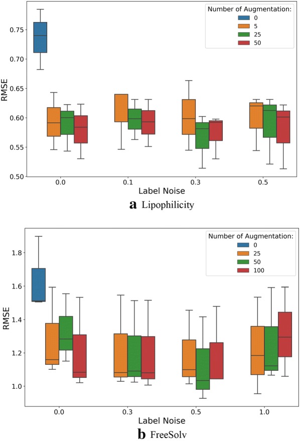
Performances of Lipophilicity models on different number of augmented SMILES per compound and Gaussian Noise (σnoise) added to the original experimental values
The results above show one limitation of using SMILES as input for deep learning model: the model actually learns to map individual SMILES to molecular properties/activities instead of linking actual molecular structures to their properties/activities. However, the SMILES augmentation is used as a regularization technique, making the model more robust to various SMILES representation for the same molecule. Appropriately adding random label noise to the augmented SMILES led to improved predictive power of the regression model. For the same data augmentation setting, testing results with TTA were found to be almost always better than the results on only canonical SMILES. While augmentation for training set can help in building models that can generalize well on new data, prediction accuracy can be further improved by TTA.
Conclusions
In this study, we introduced the MolPMoFiT, a novel transfer learning method for QSPR/QSAR tasks. We pre-trained a molecular structure prediction model (MSPM) using one million bioactive molecules from ChEMBL and then fine-tuned it for various QSPR/QSAR tasks. This pre-training + fine-tuning approach enables knowledge learned from large chemical data sets to transfer to smaller data sets, thereby improving the model performance and generalization. Without endpoint-specific hyperparameter tuning, this method showed comparable or better results compared to that of the state-of-the-art results reported in the literature for four benchmark datasets. In addition to the strong out-of-box performance, this method reuses the pre-trained MSMP across QSPR/QSAR tasks so that reduces the burden of hyperparameters tuning and model training. We posit that transfer learning techniques such as MolPMoFiT could significantly contribute in boosting the reliability of next-generation QSPR/QSAR models, especially for small/medium size datasets that are extremely challenging for QSAR modeling.
Acknowledgements
We gratefully thank the financial support from DARPA and ARO (grant number W911NF-18-1-0315).
Abbreviations
- MolPMoFiT
Molecular Prediction Model Fine-Tuning
- QSPR/QSAR
Quantitative structure property/activity relationship
- SMILES
Simplified Molecular-Input Line-Entry System
- GCNN
Graph convolutional neural networks
- RNN
Recurrent neural network
- CNN
Convolutional neural network
- CV
Computer vision
- NLP
Natural language processing
- MLT
Multitask learning
- MSPM
Molecular structure prediction model
- ULMFiT
Universal Language Model Fine-Tuning
- AWD-LSTM
ASGD Weight-Dropped LSTM
- D-MPNN
Directed Message Passing Neural Network
- RF
Random Forest
- FFN
Feed-Forward Network
- TTA
Test-time augmentation
Authors’ contributions
XL conceived, developed and implemented the method, performed the analysis, and wrote the manuscript. DF conceived the method and wrote the manuscript. All authors read and approved the final manusceipt.
Funding
We gratefully thank the financial support from DARPA and ARO (Grant number W911NF-18-1-0315).
Availability of data and materials
The curated datasets (.smi and .csv files) and the full updated code used in this study are freely-available at: https://github.com/XinhaoLi74/MolPMoFiT.
Competing interests
The authors declare no competing financial interests.
Footnotes
Publisher's Note
Springer Nature remains neutral with regard to jurisdictional claims in published maps and institutional affiliations.
Contributor Information
Xinhao Li, Email: xli74@ncsu.edu.
Denis Fourches, Email: dfourch@ncsu.edu.
References
- 1.Cherkasov A, Muratov EN, Fourches D, et al. QSAR modeling: where have you been? Where are you going to? J Med Chem. 2014;57:4977–5010. doi: 10.1021/jm4004285. [DOI] [PMC free article] [PubMed] [Google Scholar]
- 2.Mater AC, Coote ML. Deep Learning in Chemistry. J Chem Inf Model. 2019;59:2545–2559. doi: 10.1021/acs.jcim.9b00266. [DOI] [PubMed] [Google Scholar]
- 3.Tropsha A. Best practices for QSAR model development, validation, and exploitation. Mol Inform. 2010;29:476–488. doi: 10.1002/minf.201000061. [DOI] [PubMed] [Google Scholar]
- 4.Ma J, Sheridan RP, Liaw A, et al. Deep neural nets as a method for quantitative structure-activity relationships. J Chem Inf Model. 2015;55:263–274. doi: 10.1021/ci500747n. [DOI] [PubMed] [Google Scholar]
- 5.Fourches D, Williams AJ, Patlewicz G, et al (2018) Computational Tools for ADMET Profiling. In: Computational Toxicology. pp 211–244
- 6.Li X, Kleinstreuer NC, Fourches D. Hierarchical quantitative structure-activity relationship modeling approach for integrating binary, multiclass, and regression models of acute oral systemic toxicity. Chem Res Toxicol. 2020;33:353–366. doi: 10.1021/acs.chemrestox.9b00259. [DOI] [PubMed] [Google Scholar]
- 7.Ash J, Fourches D. Characterizing the chemical space of ERK2 kinase inhibitors using descriptors computed from molecular dynamics trajectories. J Chem Inf Model. 2017;57:1286–1299. doi: 10.1021/acs.jcim.7b00048. [DOI] [PubMed] [Google Scholar]
- 8.Fourches D, Ash J. 4D- quantitative structure–activity relationship modeling: making a comeback. Expert Opin Drug Discov. 2019 doi: 10.1080/17460441.2019.1664467. [DOI] [PubMed] [Google Scholar]
- 9.Xue L, Bajorath J. Molecular descriptors in chemoinformatics, computational combinatorial chemistry, and virtual screening. Comb Chem High Throughput Screen. 2012;3:363–372. doi: 10.2174/1386207003331454. [DOI] [PubMed] [Google Scholar]
- 10.Gilmer J, Schoenholz SS, Riley PF, et al (2017) Neural message passing for quantum chemistry. http://arxiv.org/abs/1704.01212
- 11.Chen C, Ye W, Zuo Y, et al. Graph networks as a universal machine learning framework for molecules and crystals. Chem Mater. 2019;31:3564–3572. doi: 10.1021/acs.chemmater.9b01294. [DOI] [Google Scholar]
- 12.Yang K, Swanson K, Jin W, et al. Analyzing learned molecular representations for property prediction. J Chem Inf Model. 2019;59:3370–3388. doi: 10.1021/acs.jcim.9b00237. [DOI] [PMC free article] [PubMed] [Google Scholar]
- 13.Duvenaud D, Maclaurin D, Aguilera-Iparraguirre J, et al. Convolutional networks on graphs for learning molecular fingerprints. Adv Neural Inf Process Syst. 2015;2015:2224–2232. [Google Scholar]
- 14.Coley CW, Barzilay R, Green WH, et al. Convolutional embedding of attributed molecular graphs for physical property prediction. J Chem Inf Model. 2017;57:1757–1772. doi: 10.1021/acs.jcim.6b00601. [DOI] [PubMed] [Google Scholar]
- 15.Wu Z, Ramsundar B, Feinberg EN, et al. MoleculeNet: a benchmark for molecular machine learning. Chem Sci. 2018;9:513–530. doi: 10.1039/C7SC02664A. [DOI] [PMC free article] [PubMed] [Google Scholar]
- 16.Pham T, Tran T, Venkatesh S (2018) Graph memory networks for molecular activity prediction. In: Proceedings - international conference on pattern recognition. pp 639–644
- 17.Wang X, Li Z, Jiang M, et al. Molecule property prediction based on spatial graph embedding. J Chem Inf Model. 2019 doi: 10.1021/acs.jcim.9b00410. [DOI] [PubMed] [Google Scholar]
- 18.Feinberg EN, Sur D, Wu Z, et al. PotentialNet for molecular property prediction. ACS Cent Sci. 2018;4:1520–1530. doi: 10.1021/acscentsci.8b00507. [DOI] [PMC free article] [PubMed] [Google Scholar]
- 19.Stokes JM, Yang K, Swanson K, et al. A deep learning approach to antibiotic discovery. Cell. 2020;180:688–702.e13. doi: 10.1016/j.cell.2020.01.021. [DOI] [PMC free article] [PubMed] [Google Scholar]
- 20.Tang B, Kramer ST, Fang M, et al. A self-attention based message passing neural network for predicting molecular lipophilicity and aqueous solubility. J Cheminform. 2020;12:15. doi: 10.1186/s13321-020-0414-z. [DOI] [PMC free article] [PubMed] [Google Scholar]
- 21.Withnall M, Lindelöf E, Engkvist O, Chen H. Building attention and edge message passing neural networks for bioactivity and physical-chemical property prediction. J Cheminform. 2020;12:1–18. doi: 10.1186/s13321-019-0407-y. [DOI] [PMC free article] [PubMed] [Google Scholar]
- 22.Goh GB, Hodas NO, Siegel C, Vishnu A (2017) SMILES2Vec: An interpretable general-purpose deep neural network for predicting chemical properties. http://arxiv.org/abs/1712.02034
- 23.Zheng S, Yan X, Yang Y, Xu J. Identifying structure-property relationships through SMILES syntax analysis with self-attention mechanism. J Chem Inf Model. 2019;59:914–923. doi: 10.1021/acs.jcim.8b00803. [DOI] [PubMed] [Google Scholar]
- 24.Kimber TB, Engelke S, Tetko I V, et al (2018) Synergy effect between convolutional neural networks and the multiplicity of SMILES for improvement of molecular prediction. http://arxiv.org/abs/1812.04439
- 25.Goh GB, Siegel C, Vishnu A, et al (2017) Chemception: a deep neural network with minimal chemistry knowledge matches the performance of expert-developed QSAR/QSPR models. https://arxiv.org/pdf/1706.06689.pdf
- 26.Goh GB, Siegel C, Vishnu A, Hodas NO (2017) Using rule-based labels for weak supervised learning: a ChemNet for transferable chemical property prediction.
- 27.Paul A, Jha D, Al-Bahrani R, et al (2018) CheMixNet: Mixed DNN architectures for predicting chemical properties using multiple molecular representations. http://arxiv.org/abs/1811.08283
- 28.Goh GB, Siegel C, Vishnu A, et al (2018) How much chemistry does a deep neural network need to know to make accurate predictions? In: Proceedings - 2018 IEEE winter conference on applications of computer vision, WACV 2018. pp 1340–1349
- 29.Fernandez M, Ban F, Woo G, et al. Toxic colors: the use of deep learning for predicting toxicity of compounds merely from their graphic images. J Chem Inf Model. 2018;58:1533–1543. doi: 10.1021/acs.jcim.8b00338. [DOI] [PubMed] [Google Scholar]
- 30.Asilar E, Hemmerich J, Ecker GF. Image based liver toxicity prediction. J Chem Inf Model. 2020 doi: 10.1021/acs.jcim.9b00713. [DOI] [PubMed] [Google Scholar]
- 31.Varnek A, Fourches D, Hoonakker F, Solov’ev VP. Substructural fragments: an universal language to encode reactions, molecular and supramolecular structures. J Comput Aided Mol Des. 2005;19:693–703. doi: 10.1007/s10822-005-9008-0. [DOI] [PubMed] [Google Scholar]
- 32.Weininger D. SMILES, a chemical language and information system. 1. Introduction to methodology and encoding rules. J Chem Inf Model. 1988;28:31–36. doi: 10.1021/ci00057a005. [DOI] [Google Scholar]
- 33.Weininger D, Weininger A, Weininger JL. SMILES. 2. Algorithm for generation of unique SMILES notation. J Chem Inf Model. 1989;29:97–101. doi: 10.1021/ci00062a008. [DOI] [Google Scholar]
- 34.Hopfield JJ. Neural networks and physical systems with emergent collective computational abilities. Proc Natl Acad Sci. 1982;79:2554–2558. doi: 10.1073/pnas.79.8.2554. [DOI] [PMC free article] [PubMed] [Google Scholar]
- 35.Lipton ZC, Berkowitz J, Elkan C (2015) A critical review of recurrent neural networks for sequence learning. http://arxiv.org/abs/1506.00019
- 36.Kim Y Convolutional neural networks for sentence classification. http://arxiv.org/abs/1408.5882
- 37.Vaswani A, Shazeer N, Parmar N, et al (2017) Attention Is All You Need. http://arxiv.org/abs/1706.03762
- 38.Deng J, Dong W, Socher R, et al (2009) ImageNet: A large-scale hierarchical image database. In: 2009 IEEE conference on computer vision and pattern recognition. IEEE, pp 248–255
- 39.Canziani A, Paszke A, Culurciello E (2016) An analysis of deep neural network models for practical applications. http://arxiv.org/abs/1605.07678
- 40.Mikolov T, Chen K, Corrado G, Dean J (2013) Efficient estimation of word representations in vector space. http://arxiv.org/abs/1301.3781
- 41.Pennington J, Socher R, Manning CD (2014) GloVe: Global vectors for word representation. In: Empirical methods in natural language processing (EMNLP). pp 1532–1543
- 42.Joulin A, Grave E, Bojanowski P, et al (2016) FastText.zip: Compressing text classification models. http://arxiv.org/abs/1612.03651
- 43.Peters ME, Neumann M, Iyyer M, et al (2018) Deep contextualized word representations. http://allennlp.org/elmo
- 44.Devlin J, Chang M-W, Lee K, Toutanova K (2018) BERT: Pre-training of deep bidirectional transformers for language understanding. http://arxiv.org/abs/1810.04805
- 45.Howard J, Ruder S (2018) Universal language model fine-tuning for text classification. http://arxiv.org/abs/1801.06146
- 46.Yang Z, Dai Z, Yang Y, et al (2019) XLNet: Generalized autoregressive pretraining for language understanding. http://arxiv.org/abs/1906.08237
- 47.Liu Y, Ott M, Goyal N, et al (2019) RoBERTa: A robustly optimized BERT pretraining approach. http://arxiv.org/abs/1907.11692
- 48.Gaulton A, Bellis LJ, Bento AP, et al. ChEMBL: a large-scale bioactivity database for drug discovery. Nucleic Acids Res. 2012;40:1100–1107. doi: 10.1093/nar/gkr777. [DOI] [PMC free article] [PubMed] [Google Scholar]
- 49.Jaeger S, Fulle S, Turk S. Mol2vec: unsupervised Machine Learning Approach with Chemical Intuition. J Chem Inf Model. 2018;58:27–35. doi: 10.1021/acs.jcim.7b00616. [DOI] [PubMed] [Google Scholar]
- 50.Hu W, Liu B, Gomes J, et al (2019) Pre-training Graph Neural Networks. https://arxiv.org/pdf/1905.12265.pdf
- 51.Xu Y, Ma J, Liaw A, et al. Demystifying multitask deep neural networks for quantitative structure-activity relationships. J Chem Inf Model. 2017;57:2490–2504. doi: 10.1021/acs.jcim.7b00087. [DOI] [PubMed] [Google Scholar]
- 52.Sosnin S, Karlov D, Tetko IV, Fedorov MV. Comparative study of multitask toxicity modeling on a broad chemical space. J Chem Inf Model. 2019;59:1062–1072. doi: 10.1021/acs.jcim.8b00685. [DOI] [PubMed] [Google Scholar]
- 53.León A, Chen B, Gillet VJ. Effect of missing data on multitask prediction methods. J Cheminform. 2018;10:26. doi: 10.1186/s13321-018-0281-z. [DOI] [PMC free article] [PubMed] [Google Scholar]
- 54.Wu K, Wei G-W. Quantitative toxicity prediction using topology based multitask deep neural networks. J Chem Inf Model. 2018;58:520–531. doi: 10.1021/acs.jcim.7b00558. [DOI] [PubMed] [Google Scholar]
- 55.Varnek A, Gaudin C, Marcou G, et al. Inductive transfer of knowledge: application of multi-task learning and feature net approaches to model tissue-air partition coefficients. J Chem Inf Model. 2009;49:133–144. doi: 10.1021/ci8002914. [DOI] [PubMed] [Google Scholar]
- 56.Ramsundar B, Liu B, Wu Z, et al. Is multitask deep learning practical for pharma? J Chem Inf Model. 2017;57:2068–2076. doi: 10.1021/acs.jcim.7b00146. [DOI] [PubMed] [Google Scholar]
- 57.Merity S, Xiong C, Bradbury J, Socher R (2016) Pointer sentinel mixture models. http://arxiv.org/abs/1609.07843
- 58.Linzen T, Dupoux E, Goldberg Y (2016) Assessing the Ability of LSTMs to Learn Syntax-Sensitive Dependencies. http://arxiv.org/abs/1611.01368
- 59.Gulordava K, Bojanowski P, Grave E, et al (2018) Colorless green recurrent networks dream hierarchically. http://arxiv.org/abs/1803.11138
- 60.Radford A, Jozefowicz R, Sutskever I (2017) Learning to generate reviews and discovering sentiment. http://arxiv.org/abs/1704.01444
- 61.Merity S, Keskar NS, Socher R (2017) Regularizing and optimizing LSTM language models. http://arxiv.org/abs/1708.02182
- 62.Hochreiter S, Schmidhuber J. Long short-term memory. Neural Comput. 1997;9:1735–1780. doi: 10.1162/neco.1997.9.8.1735. [DOI] [PubMed] [Google Scholar]
- 63.Smith LN (2018) A disciplined approach to neural network hyper-parameters: Part 1: learning rate, batch size, momentum, and weight decay. http://arxiv.org/abs/1803.09820
- 64.Yosinski J, Clune J, Bengio Y, Lipson H (2014) How transferable are features in deep neural networks? In: Advances in neural information processing systems. pp 3320–3328
- 65.Adam P, Sam G, et al (2017) Automatic differentiation in PyTorch. In: 31st Conf Neural Inf Process Syst (NIPS 2017)
- 66.Howard J, Gugger S. Fastai: a layered API for deep learning. Information. 2020;11:108. doi: 10.3390/info11020108. [DOI] [Google Scholar]
- 67.Swain M MolVS: Molecule validation and standardization. https://github.com/mcs07/MolVS
- 68.Landrum G RDKit: Open-source cheminformatics. http://www.rdkit.org
- 69.Fadaee M, Bisazza A, Monz C (2017) Data augmentation for low-resource neural machine translation. http://arxiv.org/abs/1705.00440
- 70.Kobayashi S (2018) Contextual Augmentation: Data Augmentation by Words with Paradigmatic Relations. In: Proceedings of the 2018 Conference of the North American Chapter of the Association for Computational Linguistics: Human Language Technologies, Volume 2 (Short Papers). Association for Computational Linguistics, Stroudsburg, PA, USA, pp 452–457
- 71.Kafle K, Yousefhussien M, Kanan C (2017) Data Augmentation for Visual Question Answering. In: Proceedings of the 10th international conference on natural language generation. association for computational linguistics, Stroudsburg, PA, USA, pp 198–202
- 72.Lei C, Hu B, Wang D, et al (2019) A preliminary study on data augmentation of deep learning for image classification. In: ACM International Conference Proceeding Series
- 73.Bjerrum EJ (2017) SMILES enumeration as data augmentation for neural network modeling of molecules. http://arxiv.org/abs/1703.07076
- 74.Arús-Pous J, Blaschke T, Ulander S, et al. Exploring the GDB-13 chemical space using deep generative models. J Cheminform. 2019;11:20. doi: 10.1186/s13321-019-0341-z. [DOI] [PMC free article] [PubMed] [Google Scholar]
- 75.Arús-Pous J, Johansson SV, Prykhodko O, et al. Randomized SMILES strings improve the quality of molecular generative models. J Cheminform. 2019;11:71. doi: 10.1186/s13321-019-0393-0. [DOI] [PMC free article] [PubMed] [Google Scholar]
- 76.Cortes-Ciriano I, Bender A. Improved chemical structure-activity modeling through data augmentation. J Chem Inf Model. 2015;55:2682–2692. doi: 10.1021/acs.jcim.5b00570. [DOI] [PubMed] [Google Scholar]
- 77.Sheridan RP. Time-split cross-validation as a method for estimating the goodness of prospective prediction. J Chem Inf Model. 2013;53:783–790. doi: 10.1021/ci400084k. [DOI] [PubMed] [Google Scholar]
Associated Data
This section collects any data citations, data availability statements, or supplementary materials included in this article.
Data Availability Statement
The curated datasets (.smi and .csv files) and the full updated code used in this study are freely-available at: https://github.com/XinhaoLi74/MolPMoFiT.


