Accurate Multiobjective Design in a Space of Millions of Transition Metal Complexes with Neural-Network-Driven Efficient Global Optimization

Abstract

The accelerated discovery of materials for real world applications requires the achievement of multiple design objectives. The multidimensional nature of the search necessitates exploration of multimillion compound libraries over which even density functional theory (DFT) screening is intractable. Machine learning (e.g., artificial neural network, ANN, or Gaussian process, GP) models for this task are limited by training data availability and predictive uncertainty quantification (UQ). We overcome such limitations by using efficient global optimization (EGO) with the multidimensional expected improvement (EI) criterion. EGO balances exploitation of a trained model with acquisition of new DFT data at the Pareto front, the region of chemical space that contains the optimal trade-off between multiple design criteria. We demonstrate this approach for the simultaneous optimization of redox potential and solubility in candidate M(II)/M(III) redox couples for redox flow batteries from a space of 2.8 M transition metal complexes designed for stability in practical redox flow battery (RFB) applications. We show that a multitask ANN with latent-distance-based UQ surpasses the generalization performance of a GP in this space. With this approach, ANN prediction and EI scoring of the full space are achieved in minutes. Starting from ca. 100 representative points, EGO improves both properties by over 3 standard deviations in only five generations. Analysis of lookahead errors confirms rapid ANN model improvement during the EGO process, achieving suitable accuracy for predictive design in the space of transition metal complexes. The ANN-driven EI approach achieves at least 500-fold acceleration over random search, identifying a Pareto-optimal design in around 5 weeks instead of 50 years.

Short abstract

Multiobjective optimization with artificial neural networks enables computational discovery of top new materials from millions of candidates in weeks instead of decades.

Introduction

The discovery of new functional materials is essential to address outstanding challenges in energy and resource utilization. Computational screening, e.g., with first-principles density functional theory (DFT), is a powerful complement to experimental efforts due to the ease and speed with which properties can be evaluated. Materials design often necessitates that multiple objectives be satisfied, such as meeting an energetic criterion while also exhibiting stability or low cost.¹ In these cases, it is beneficial to optimize properties along a Pareto front, the region of chemical space that contains the optimal trade-offs between desired properties, as has occasionally been carried out in chemistry,²⁻⁶ e.g., for catalyst design.² Simultaneous achievement of multiple design objectives to locate the Pareto front mandates exploration of vast chemical spaces (ca. millions of candidates), for which even efficient physics-based modeling is intractable.

In recent years, machine learning (ML) has emerged as a promising alternative to direct, physics-based simulation by enabling property prediction in seconds that would normally take days or weeks for full DFT-based evaluation.^1,7 Although ML models were first demonstrated to achieve near-DFT accuracy in small molecule organic chemistry,⁸ recent developments have focused on challenging materials spaces, such as transition metal chemistry^7,9−16 and inorganic materials.¹⁷⁻²² Challenges remain to deliver on the promise of ML-accelerated materials discovery. Prior to property prediction, ML models still require substantial training data, typically on the order of thousands^23,24 to millions^25,26 of DFT-evaluated properties. Even when such models are carefully trained, performance on a set aside test set can differ^10,14,27,28 from the true generalization performance on out-of-sample compounds that are the typical target of discovery efforts.

Active learning has been recognized^5,29−37 as an attractive paradigm for balancing between data acquisition in ML model training (i.e., exploration) and ML-model-based prediction (i.e., exploitation). Within chemical discovery,^5,30−37 Bayesian optimization^38,39 approaches, such as efficient global optimization (EGO) with the expected improvement (EI) criterion,³³⁻³⁷ have begun to be employed to balance exploration with exploitation. In cases where model uncertainty quantification (UQ) is possible, these approaches have been fruitfully applied to accelerate ML model training²⁹ and single-objective discovery efforts³³⁻³⁷ but not yet to large-scale multiobjective design challenges.

In this work, we develop an ML- and DFT-driven multiobjective transition metal complex design workflow and apply it to redox flow battery (RFB) redox couple discovery. RFBs^40,41 decouple power delivery and cell capacity by storing the redox-active species separately and delivering or replacing them on demand, making RFBs ideal for economical, large-scale energy storage.^42,43 Transition metal ions (e.g., vanadium) or complexes have been widely used in RFBs due to their ability to cycle through a range of oxidation states. However, smaller transition metal complexes with high redox potentials tend to diffuse across the membrane in a phenomenon known as crossover. Complexation with bulkier organic ligands can both tune redox properties and prevent diffusion,⁴⁴ but these same ligands can limit solubility⁴⁵ in the polar, organic solvents (e.g., acetonitrile) favored for RFB electrolytes.

Computational optimization of transition metal complex redox couples for RFBs should therefore address crossover, stability, solubility, and redox potential. We address the first two challenges by constructing a 2.8 M compound space of 700k candidate bulky ligands that are expected to form stable complexes with four open shell transition metal ions. To optimize solubility and redox potential within this space, we then employ two-dimensional EI to balance exploration and exploitation at the Pareto front. We show that a multitask ANN with latent-distance-based UQ metrics¹⁴ generalizes better than a Gaussian process, achieving good predictive accuracy from a combination of data sets from prior work^7,9,10,13 and representative points from the design space. This active learning approach rapidly improves properties and model prediction errors in only a handful of generations, revealing design rules for RFB redox couples satisfying multiple objectives. The ANN-driven EI approach achieves at least 500-fold acceleration over random search, identifying a Pareto-optimal design in weeks instead of decades.

Results and Discussion

Design Space and Objectives

We begin by reviewing the multiple concerns we must address in the design of transition-metal complex-based redox couples for RFBs. To address the challenges of crossover and stability, we created a diverse complex space of nearly three million unique candidate redox couples with bulkier ligands that are expected avoid the problem of crossover (Figure 1). This space was created through a series of hierarchical steps that started with core heterocyclic ligands inspired by experiment^46,47 that we subsequently modified, optionally joined, and functionalized. By using experimentally inspired design rules for heterocycle construction, we anticipated that these ligands would form stable complexes and validated this expectation with DFT calculations. In an application where stability was the paramount concern, an estimate of stability could instead be added as an explicit objective to the multiobjective optimization. Nitrogen or oxygen atoms act as the metal-coordinating atoms in eight distinct five- or six-membered heterocycles, and further modification (e.g., insertion of NH, S, O, or a C–C double bond) of the nonmetal-coordinating ring structure produced 38 nonredundant heterocycles (Figure 1 and Figure S1). Along with the monodentate core ligands (including pyridine, furan, and oxazole), we fused all possible heterocycle combinations into 741 bidentate ligands by forming a carbon–carbon bond between sites adjacent to the metal-coordinating atom (Figure 1 and Figure S1).

Figure 1.

Approach for hierarchical assembly of a 2.8 M homoleptic complex design space for multiobjective RFB design. The sequential stages that lead to each combinatorial step are indicated in the flowchart at left starting with selection and modification of rings, optionally fusing them to form 779 unique monodentate and bidentate ligands, functionalization of ligands with 897 unique functional groups, and finally complexation with four metals. At right, example skeleton structure components and their assembly or modification coinciding with each step are shown to form a bidentate oxygen-coordinating (coordinating atoms shown with red or blue highlight) ligand. The functional group assembly step is indicated in the black inset with the resulting structure shown. Finally a ball and stick structure is shown for an assembled complex.

To ensure a smoothly varying space for property fine-tuning, core ligands were hierarchically functionalized three bonds away from the metal-coordinating atom (i.e., para in the six-membered rings, Text S1). Methylene or phenyl groups were sequentially added up to two times, optionally functionalized (i.e., for methylene only) with up to two functional groups (e.g., OH, NH₂, or CH₃), and finally capped with a terminal functional group (e.g., Cl, OH, or NH₂) for a total of 897 functionalizations (Figure 1 and Figure S2 and Text S1). These functionalizations were added symmetrically to all ligands, producing approximately 700k distinct ligands that form 2.8 M unique homoleptic complexes with four transition metals (Figure 1 and Text S1). Although synthetic accessibility is paramount for experimental realization of a single Pareto optimal design, the advantage of our combinatorial approach is that it gives rise to a smoothly varying space that has the promise of allowing optimization algorithms to reveal design motifs while remaining consistent with previously experimentally characterized^46,47 complexes.

The performance of an RFB is determined by the cell voltage, E_cell, which is affected by both the redox potential of the redox couple as well as its concentration in the RFB electrolyte:

1

where ΔG_ox(sol) is the Gibbs free energy of the oxidation or reduction process, n is the number of electrons ionized, F is Faraday’s constant, and C is the concentration of the redox active species in the electrolyte.

We thus focus on optimizing in our complex space the remaining two design objectives: (i) maximizing redox potential and (ii) maximizing solubility. As in prior work,^9,11 the ionization process we optimize was computed from the ground state of the solvated M(II) (M = Cr, Mn, Fe, or Co) complex to the lowest energy M(III) complex that differs by loss of a single spin-up or spin-down electron (see Methods and Table S1). The ΔG_ox(sol) of each redox couple was modeled as a one-electron ionization of the M(II) complex:

2

evaluated as the gas phase adiabatic ionization potential combined with single point solvation free energy corrections (see Methods). To estimate solubility⁴⁸ in polar solvents, we computed the standard hydrophilicity or logP (i.e., partition coefficient between octanol and water) from the ground state M(II) complex as

3

where the numerator and denominator both correspond to solvation free energies (see Methods). To ensure computational efficiency, we modeled solvent effects implicitly with a thermodynamic cycle approach, neglected vibrational corrections, and combined hybrid DFT with a modest, polarized double-ζ basis set (Figure S3, see Methods). These choices both allowed us to leverage data sets of transition metal complexes from prior work^7,9,10,13 and rapidly uncover design principles.

Optimization Approach

To identify potential lead compounds in the design space, we used the expected improvement (EI) criterion,⁴⁹ widely employed³³⁻³⁷ for optimization with probabilistic surrogate models. EI ranks data points based on how much they are likely to improve on the current best characterized point, emphasizing uncertain points based on the model used to make these predictions. For one-dimensional minimization, the simplest acquisition function (i.e., a way to quantify the priority with which we should evaluate a point, x) corresponds to the expected decrease in the value of the objective, or improvement, I:

4

at a point x with estimated value ŷ(x) (i.e., from a model prediction) relative to the current best design, x*, with known value y(x*). The expected improvement acquisition function is evaluated as

5

where p_x (ŷ) is the distribution of model predictions. When the distribution is Gaussian with mean value μ(x) with variance σ²(x), one can obtain an analytical integral of eq 5 in an approach known as efficient global optimization⁴⁹ (EGO).

Within EGO, the EI acquisition function at every new point x is then:

6

where Φ and φ are the cumulative and distribution functions of the standard normal distribution. The Φ term, also referred to as the probability of improvement (i.e., P[I]), encourages exploitation of the model, whereas the second term favors exploration of high uncertainty points.

While 1D EGO has proven useful in accelerating chemical design,^33,34 RFB redox couple design considerations are inherently multifaceted. To consider multiple design objectives, we must define a Pareto front of the best possible trade-offs⁵⁰ between high redox potential (i.e., high ΔG_ox(sol)) and solubility (i.e., lower logP) in the design space (Figure 2). We therefore extended the two-dimensional EI^51,52 approach to chemical design (Algorithm S1). In 2D EI, the improvement is defined as the Euclidean distance a point x lies beyond the current Pareto front, and the total probability mass beyond the front defines E[I] (Figure 2). For this approach, we need a ML-model predicted distribution of the ΔG_ox(sol) and logP values for a new complex

7

where μ̂_ΔGox(sol) and μ̂_logP are the predicted mean values and σ̂_ΔGox(sol)² and σ̂_logP are the effective variances. Analytical expressions for the 2D EI integrals similar to eq 6 have been derived⁵² for these independent, Gaussian distributions by approximating the distance to the front from the distance to the nearest explicit point of the front (Algorithm S1).

Figure 2.

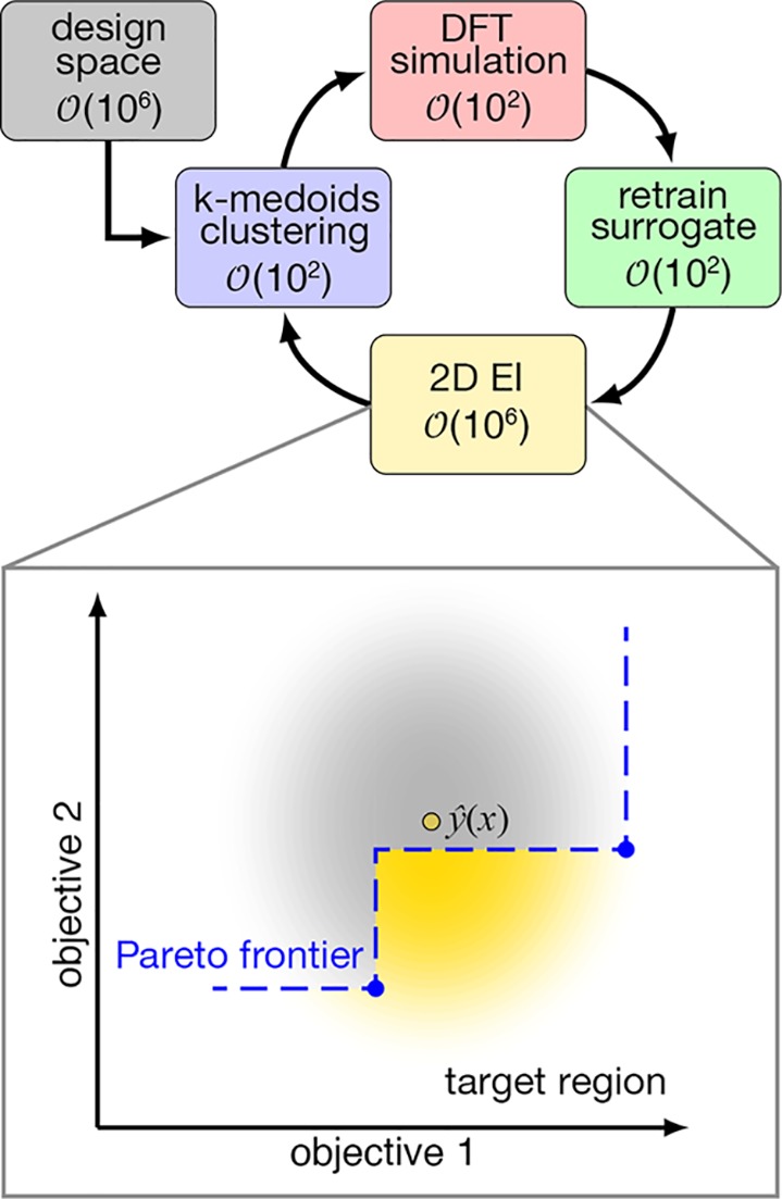
Illustration of the active learning workflow used in this work to explore a 2.8 M-complex space. DFT simulations are performed on approximately 100 cluster medoids, which are used to iteratively train ML surrogate models. The surrogate models score all possible 2.8 M candidates using 2D expected improvement (EI), and the top scoring complexes are clustered to repeat the process. Inset: illustration of a Pareto set (blue points) and front (dashed line) for a 2D objective function. The distribution of property values at trial point ŷ(x) (yellow outlined circle) is shown, and the probability mass below the front is shown in yellow.

Machine Learning Models

To use 2D EI for accelerated exploration, we require a surrogate model capable of rapidly predicting properties that generalizes well across a 2.8 M compound design space as well as a quantitative uncertainty metric. A Gaussian process (GP) provides inherent uncertainty estimates from the structure of the learned posterior distribution⁵³ that are suitable for EGO, but ANNs do not. We recently developed an uncertainty quantification metric for ANNs¹⁴ based on the distance of a point to training data in the latent space (i.e., the distribution of the data after transformation by the ANN). This metric both demonstrated superior performance to commonly employed (i.e., ensemble variance) estimates^29,54 in active learning experiments and did not require the cost of training multiple models. To convert the latent space distance, d, to the units of property prediction, we modeled the generalization error with a conditionally Gaussian distribution:

8

where σ₁ and σ₂ are parameters obtained from maximum likelihood estimation on a small (10%) set of out-of-sample complexes (Figure S4). Thus, our error distribution can be treated as Gaussian for both ANNs and GPs, reducing the choice of ML model in EGO to the one with the best generalization performance.

We therefore trained and compared GPs and single-task (ST) ANN models to independently predict DFT values of ΔG_ox(sol) and logP as well as a multitask (MT) ANN trained to predict both ΔG_ox(sol) and logP. All ML models were trained on revised autocorrelations (RACs),⁹ a molecular graph-based representation (see Methods). RACs are tailored for open-shell transition metal chemistry^9,11,12,16 and have demonstrated modest errors (ca. 0.2–0.3 eV) in combination with kernel or neural network models on small data sets (ca. 200–300 points) of redox/ionization potentials.^9,12 Notably, this representation incorporates no geometric information, which enables rapid (ca. 3 min) ML-model assessment and uncertainty quantification of the 2.8 M-complex design space but precludes prediction of property conformational dependence (Text S2).

To compare the baseline prediction accuracy of GP and ANNs, we assembled a data set of 235 predominantly heteroleptic transition metal (M = Cr, Mn, Fe, or Co) complexes from prior work^7,9,10,13 (i.e., “hot start” data) and assessed train/test errors from a 90/10 split (see Methods and Figure S5 and Table S2). For ΔG_ox(sol), training mean absolute errors (MAEs) are low across all models (ST: 0.11, MT: 0.15, and GP: 0.13 eV). The ST ANN has fewer outliers, as evidenced by a lower training root-mean square error (RMSE) than the other two models (Table S3). As expected, all test MAEs are higher, with the MT ANN performing the best (0.32 eV MAE), consistent with some prior observations on MT ANNs⁵⁵ (Figure 3 and Table S3). For logP, training MAEs are lowest for the GP (ST: 1.45 × 10^–4, MT: 1.45 × 10^–4, and GP: 1.05 × 10^–4), the ST ANN produces the lowest test error (1.49 × 10^–4), and all train/test MAEs are relatively modest (Tables S3–S4 and Figure S6). In addition to better performance of the ANNs, latent distance enables superior error control for the MT ANN with respect to variance in the GP for ΔG_ox(sol) prediction: excluding the five highest uncertainty points reduces MAE from 0.32 to 0.21 eV for the ANN vs 0.45 to 0.34 eV for the GP. Already low logP test MAEs are not significantly improved by any uncertainty-based metric (Figure S7).

Figure 3.

(Top, left) Generalization performance of multitask ANN (green bars), single task ANN (blue bars), and GP models (gray bars) for ΔG_ox(sol) (left) and logP (right). Train and test logP errors are also shown in an expanded inset. (Bottom, left) Distribution of properties between “hot start” (in red) and clustered representative (generation 1, in orange) data set. (Right) Principal component analysis in RAC-155 of the full design space (binned histogram, colored according to inset color bar), the original “hot start” data (red circles), and representative clusters (generation 1, orange circles).

As a test of model generalization, we evaluated the performance of the models trained on “hot start” data to predict properties of design space complexes. It is evident from principal component analysis in the RAC representation that the “hot start” data and design space compounds have limited overlap (Figure 3). The “hot start” data consist of smaller, lower symmetry complexes with low-denticity ligands as compared to the homoleptic complex space, which give them relatively high redox potentials but make them unsuitable for applications in RFBs (Figure 3 and Figure S8). To identify the model with the best generalization characteristics, we carried out diversity-oriented clustering on the complete design space and obtained DFT properties of a representative set of 107 transition metal complexes (see Methods). As expected, MAEs are significantly higher for all models (2–3x for ΔG_ox(sol) and 1–2 orders of magnitude for logP) on this representative set than the corresponding test MAEs (Figure 3 and Table S3 and Figure S6). Among the model choices, the MT ANN distinguishes itself by exhibiting the lowest generalization errors for both ΔG_ox(sol) (MT: 0.71 eV, ST: 0.80 eV, GP: 1.47 eV) and logP (MT: 3.04 × 10^–3, ST: 5.92 × 10^–3, GP: 1.31 × 10^–2) properties (Figure 3 and Tables S3–S5 and Figure S6). While the representative data set properties differ significantly from the “hot start” data for both ΔG_ox(sol) and logP, poorer generalization of the logP models can likely be attributed to the more substantial differences in the logP distributions of the two data sets than ΔG_ox(sol) (Figure 3). Both GP and ANN UQ metrics can be used to isolate higher error points, and all metrics identify higher prediction uncertainty for the representative members of the design space than for the “hot start” data test partition (Figure S9). Because of its superior generalization, we selected the MT ANN for multiobjective expected improvement optimization of redox couples.

Design Outcomes

At the start of the expected improvement optimization, we used the 107-complex representative data set to define our initial Pareto front (Figure 4). This Pareto front, i.e., the set of known compounds that represents the current best combination of ΔG_ox(sol) and logP, consisted of six points formed from three of the metals (i.e., Fe, Co, or Mn) complexed with bidentate ligands (Figure 4). An 82-atom, low-spin Fe complex with a nitrogen-coordinating bidentate ligand had the best (i.e., lowest) logP of −5.31 × 10^–2 (ΔG_ox(sol) = 6.36 eV), likely due to the ligand’s functionalization with a large number of strongly polar groups (i.e., chloride and carbonyl) (A in Figure 4). A 145-atom, high-spin Mn complex with an oxygen-coordinating bidentate ligand had the highest ΔG_ox(sol) of 7.37 eV (logP = −4.38 × 10^–2) in the initial data set (B in Figure 4). The other four Pareto complexes naturally represent a trade-off of the two quantities between these limits.

Figure 4.

ANN-predicted logP and ΔG_ox(sol) values for the 2.8 M-complex design space. The ANN has been trained on representative clusters and “hot start” data. The generation 1 data (blue diamonds) forming the Pareto front (blue line) are shown in both panes. The best (i.e., lowest) logP Fe complex (A) and highest ΔG_ox(sol) Mn complex (B) are labeled at left and shown at top. The points are colored by the probability of improving on the front (P[I], left) or expected improvement (E[I], right). On the basis of the approximation of the front used in the E[I], potential complexes equidistant between points on the front score highest. The 100 selected cluster medoids (yellow triangles) from the 10k top E[I]-scoring complexes selected for subsequent DFT calculations are indicated at right, with two examples, a Co complex (C) and Mn complex (D), shown at top right. All representative complexes are shown in both 3D sticks and with each ligand shown as a skeleton structure.

We then retrained the MT ANN and calibrated its UQ metric on both “hot start” and the representative data set and refer to this as the generation 1 ANN model (Figure 2 and Figure S10, also see Methods). Using the generation 1 model, we evaluated the probability that each candidate in the 2.8 M complex design space would improve on the Pareto front (i.e., P[I]), as well as the associated expected improvement (E[I]). While the P[I] uniformly favors any point predicted by the ANN to be beyond the front, the E[I] focuses on the region of the front that will lead to the largest possible property improvement (Figure 4). In conventional EGO, only the top-scoring candidate would be selected, but due to the parallel nature of our calculations we clustered the top-scoring complexes to obtain representative points for characterization with DFT in order to generate additional data for model retraining (Figures 2 and 4, also see Methods). After only a single iteration, the top-scoring complexes making up the Pareto front indeed were primarily comprised of these new generation 2 complexes (Table S6).

Carrying out this optimization requires balancing computationally demanding DFT calculations at each generation (i.e., over a week of wall time for 100 complexes) with the much more rapid ANN-derived assessment of the full design space (i.e., 2.8 M complexes in ca. 3 min, Text S2 and Table S7). While there is no universal standard for stopping EGO, we chose to stop after four generations, supported in part by the rapid decline of mean E[I] values of clustered points from the top lead complexes (i.e., 10k of 2.8M) from generation 1 (mean E[I] = 0.45) to generation 4 (mean E[I] = 0.04, Figure S11). We can also assess if the model predictive power is improving during this process, given the small but growing size of the DFT training data with each generation (Table S8). To quantify model improvement, we calculated the “lookahead” errors of models trained in one generation on data from later generations. Although the model trained only on “hot start” data (i.e., generation 0) exhibits the poorest MAEs for both ΔG_ox(sol) and logP on later generation (i.e., 3–5) data sets, model prediction accuracy for both quantities improves most significantly (>50% reduction) with the incorporation of generation 1 data (Figure 5 and Tables S9–S10 and Figure S12). These lookahead MAEs generally do not improve substantially beyond generations 2–3, leveling off to values slightly above test MAEs, which is expected since EI favors points for which the model is least certain. Thus, motivated by the diminishing returns for both improving model accuracy and the likelihood of pushing the Pareto front further, as judged through the model estimates, we terminated our 2D-EI design space exploration after evaluating E[I] four times (i.e., five DFT data set generations, see Figure S10).

Figure 5.

Mean absolute errors (MAEs) for ΔG_ox(sol) (top, in eV) and logP (bottom) predictions with a multitask ANN. Each bar is colored by the generation at which it is trained, as indicated in the top inset (here, generation 0 corresponds to “hot start” data only). Lookahead MAEs are reported on data sets (1–5, as indicated on axis) generated in each relevant subsequent generation. The MAEs on a separately collected random test set representative of the full design space (random, as indicated on axis) for all multitask ANNs are also reported.

Over each generation of EI, new points were added to extend beyond the previous generation’s Pareto front. The final Pareto front consists of eight complexes, all from the last three generations of the EGO run (Figure 6 and Table S6). The direction of improvement evolved during EGO, with improvements to ΔG_ox(sol) primarily occurring in generations 2 and 3 (Figure 6). Conversely, the later generations 3–5 capture more logP improvements as ΔG_ox(sol) increases diminish, with the six best (i.e., lowest) logP values occurring in these three generations (Figure 6). Although the DFT-evaluated Pareto front moves out at each generation, the improvements are indeed diminishing, consistent with a decrease in model-predicted E[I] values (Figure 6 and Figure S11).

Figure 6.

(Left) ΔG_ox(sol) and logP values for complexes simulated during five generations of the design algorithm, colored by generation and with unique symbols for each metal center (as indicated in inset legend). The range of values sampled in each generation is indicated by a translucent convex hull, and the final Pareto front is indicated by a red line. Three complexes along this front are labeled and shown at top in both 3D sticks and with each ligand shown as a skeleton structure: the highest ΔG_ox(sol) Mn complex (A), the best trade-off Mn complex (B), and the highest logP Fe complex (C). (Right) Distribution of ΔG_ox(sol) (top) and logP (bottom) values for each generation (colors and symbols as in left pane) alongside a random sample (gray symbols). The mean value for each generation is indicated with a blue horizontal line.

Broad chemical trends are evident in the evolution of the Pareto front during EGO. While the ligands in our design space support both high and low spin redox couples, only high-spin and predominantly Mn complexes were favored in later generations, consistent with some prior observations on smaller-scale, redox-focused computational screening.⁵⁶ One confounding effect in this process is that both time limits and calculation quality criteria prevented all attempted DFT calculations suggested by the model from succeeding and being incorporated into subsequent generations (Tables S7–S8). However, we note there was no metal-dependence in the success rates, meaning that the model acquired information both from “hot start” data and from the generation 1 diversity-oriented points that informed the model’s preference for high-spin Mn complexes (Figure S13). In fact, a high-spin iron complex also appeared in the Pareto front at generation 5 because it had a lower logP (−5.60 × 10^–2) than any prior sampled complex (C in Figure 6). The highest ΔG_ox(sol) complex was a Mn complex with a bidentate oxygen-coordinating ligand with sulfur in the ring, and its polar groups also led to a better logP (−4.46 × 10^–2) than previous generations’ high-ΔG_ox(sol) complexes (A in Figure 6). Assuming equal importance of improving both properties, the highest redox potential (ΔG_ox(sol) = 8.05 eV) with good solubility (logP = −5.52 × 10^–2) at the Pareto front was observed for another high-spin Mn/O complex (complex B in Figure 6).

Commonalities are evident in the ligand structures of the Pareto front high spin Mn complexes with the highest ΔG_ox(sol) values ranging from 8.05–8.51 eV (Figure 7). All contain oxygen-coordinating bidentate ligands with a combination of a six- and a five-membered ring, with at least one ring incorporating a sulfur heteroatom (Figure 7 and Figures S14–S15). The EI process generally avoided selecting nitrogen-coordinating ligands or in-ring modification with nitrogen because these complexes were outperformed by oxygen-coordinating structures with sulfur in-ring modifications (Figure 7 and Figure S1 and Table S6). A Pareto set complex after generation 3 with high ΔG_ox(sol) (8.24 eV) did have in-ring nitrogen-modification but also significantly lower logP (−4.61 × 10^–2) than other complexes (Table S6). As with metal-dependence, all core ligand types were sampled in early generations but the optimization quickly converged toward a few select heterocycles in later generations (Figure 7 and Figures S16–S17).

Figure 7.

Composition of the eight complexes in the final Pareto set. Each complex consists of one metal center with bidentate ligands assembled from one six-membered and one five-membered ring with the metal-coordinating atom corresponding to the left-most oxygen atom. In all cases, a functional group (indicated in rounded rectangles) is attached symmetrically to both heterocycles. Each complex is represented by a unique path from left (metal center) to right (functional group), and the path is colored by whether the complex has a relatively improved logP (low logP, yellow) or ΔG_ox(sol) (high ΔG_ox(sol), blue), as indicated in the inset color bar.

The EI process most frequently selected Mn complexes that were uniformly smaller (ca. 90 atoms) than the initial diversity-oriented Pareto front complexes (ca. 120 atoms) in size (Table S6). This smaller complex size is consistent both with prior observations^9,11 that smaller complexes have higher redox potentials and the fact that the highest logP iron complex noted earlier is both the largest (184 atoms) and lowest ΔG_ox(sol) of all complexes in the final Pareto front. Since high solubility appears to be heavily influenced by the presence and nature of polar functional groups, the EI scoring likely favors atom economy (i.e., low molecular weight) to maintain high redox potential while introducing groups that can improve solubility (Figure 7). Although most of the Pareto set complexes are large, they are comparable in size to those that have been previously studied experimentally⁴⁵ for RFB applications. The polar carbonyl oxygen and hydroxyl groups were most favored in the optimization along with chloride termination, especially on methylene group backbones, but a wide range of functionalizations were sampled during optimization (Figure 7 and Tables S6 and S11). Comparing two Pareto front complexes with the same core ligand, we observe that adding more polar functional groups (e.g., amine, carbonyl, and chloride vs only carbonyl addition) does sometimes lead to significant logP enhancement (−4.49 × 10^–2 vs −4.96 × 10^–2), albeit with a reduction in the ΔG_ox(sol) (ca. 0.3 eV, Table S12). Overall, EGO using the EI criterion appears to have converged on key design elements to maximize redox potential while not limiting solubility.

Performance Evaluation

To evaluate the efficiency and accuracy of the ANN-based EGO in the design space, we compared observations made on a uniform random sample of the space (i.e., distinct from our initial diversity-oriented clustering, Figure 5, Table S8, and see Methods). Within EGO using the EI criterion, surrogate model errors could lead to poor prediction accuracy with simultaneous overconfidence causing specific areas of the design space to never be sampled with DFT calculations, as the surrogate model becomes myopically focused on the first initially promising region of chemical space. To assess this, we evaluated errors of each generation’s ANN model on this 122-complex random set (Figure 5). After rapid reduction in MAEs for both properties from the incorporation of generation 1 data (ΔG_ox(sol) gen. 0: 0.70 eV, gen. 1: 0.41 eV, gen. 5: 0.38 eV), random set MAEs remained above test MAEs but comparable to or lower than generation 5 lookahead errors (Figure 5 and Tables S9–S10). Since the random set more evenly covers the space while the EI criterion emphasized acquisition of points in one region of the design space, the low errors on the random set are encouraging evidence of the model maintaining similar accuracy across the full space to that obtained at the Pareto front. However, because this optimization procedure relies on a surrogate model, it is not guaranteed that the model-identified compounds will be optimal when evaluated with DFT.

To quantify optimization efficiency, we compared the distribution of properties observed in the 122-complex random set with the 8 complexes that form the Pareto front after five generations of EI (Figure 6 and Figures S18–S21, Tables S13–S15, and Text S3). The random set redox potentials are significantly lower than those of the Pareto complexes, with an average ΔG_ox(sol) of 5.80 eV (Figure 6). The mean logP for the random set of −4.45 × 10^–2 also indicates poorer solubility characteristics. Of the 84 complexes characterized through E[I]-based selection, nearly one-third (26) have a higher ΔG_ox(sol) than the highest value observed in the random set, four have a lower logP than the lowest random set value, and none of the random set would lie on the generation 5 Pareto front. Design principles evident from the EI generations, such as large polar-group-functionalized phenyl rings for the lowest logP or smaller (ca. 100-atom) complexes for the highest ΔG_ox(sol), are also consistent with observations from the random set (Table S15).

Overall, the generation 5 Pareto set complexes correspond to over 4 standard deviations (std. dev.) below the mean of the random set for improved solubility characteristics (logP random set std. dev. = 2.75 × 10^–3) and 3 std. dev. above the mean for random set redox properties (ΔG_ox(sol) random set std. dev. = 0.89 eV). Since the ΔG_ox(sol) and logP random set properties are not normally distributed and are more concentrated at the mean, any distribution-based analysis will provide a conservative estimate of the EI approach’s efficiency and performance (Figure S19). Assuming the two properties are independent, this analysis suggests at least a 500-fold acceleration of EGO with 2D-EI over a random search, consistent with or exceeding prior applications of EGO in chemical discovery^30,34 (Figure S19). That is, a fully random search would be expected to require 500 times as many DFT calculations to identify the same number of top performing compounds obtained with the EI approach. Given that EGO required around 4–6 weeks of parallel GPU-accelerated computation using all available (here, 64) GPUs to acquire all of the DFT properties on these large transition metal complexes, this time favorably compares to approximately 50 years for a similarly parallelized random search (Text S2 and Table S7).

Interestingly, one complex from the random set featuring a bidentate nitrogen-coordinating ligand in complex with high-spin Co had a better ΔG_ox(sol) value (7.9 eV) than the best Co/N complex sampled during EGO (Tables S6 and S15). This suggests that improvements to initial sampling of the space could benefit the optimization strategy. Future improvements could also leverage recently developed ML models⁵⁷ to predict when EI-requested calculations will succeed, increasing yield. Overall, EGO with 2D-EI provides a targeted method of orders-of-magnitude acceleration of the discovery of optimal complexes and design rules from a compound space intractable for direct simulation.

Conclusions

We have developed a multiobjective materials design strategy applied to the accelerated discovery of candidate M(II)/M(III) redox couples for redox flow batteries that are both soluble in polar solvents and have high redox potentials. We enumerated a large 2.8 M compound space comprised of bulky ligands designed to prevent crossover while forming stable transition metal complexes in order to identify redox couples that possessed both desirable solubility and redox characteristics. Since direct calculation of the full space with DFT would have been intractable, we overcame this bottleneck by implementing efficient global optimization (EGO) with a two-dimensional expected improvement (EI) criterion to balance exploration and exploitation at the Pareto front. We showed that a recently introduced latent-distance-based UQ metric in combination with a multitask ANN provided the best combination of model generalization and quantified uncertainty, surpassing commonly employed GP models. ANN property predictions and EI scores for the full 2.8 M-complex space were obtained in minutes.

Starting from ca. 100 representative points, EGO improved both properties by over 3 standard deviations in only five generations. The best-performing redox couples from EGO were high-spin Mn complexes with oxygen-coordinating bidentate ligands that contained in-ring sulfur modifications and small, polar functional groups. In total, fewer than 200 DFT data points beyond those obtained in prior studies were needed to achieve results that improved dramatically upon both ΔG_ox(sol) and logP properties. Evaluation of lookahead ANN model errors confirmed rapid model improvement during EGO, with the ANN achieving suitable levels for predictive design in the full compound space. Analysis of the property distribution of a subsequently collected random test set suggests that the ANN-driven EI approach achieved at least 500-fold acceleration over random search. In practice, this acceleration corresponds to EGO identifying a Pareto-optimal design in approximately 5 weeks as compared to a random search that would have instead required at least 50 years. We are currently exploring how the efficiency of this search strategy is sensitive to the size of each generation. We also plan to explore natural extensions to this work in the design of earth-abundant, stable, and selective catalysts, for which multiobjective design is expected to be essential.

Methods

Data Sets and Calculation Parameters

Initial structures selected from the design space for simulation were generated with molSimplify,⁵⁸ which assembles complexes with ANN-predicted metal–ligand bond lengths^7,11 and uses OpenBabel⁵⁹ as a backend for ligand structure generation from SMILES strings. All geometry optimizations and single point energy calculations were performed with a developer version of the TeraChem⁶⁰ code. For all DFT calculations, the B3LYP hybrid generalized-gradient approximation exchange-correlation functional was employed, which in TeraChem uses the VWN1-RPA form for the LDA component of the correlation energy. The LANL2DZ effective core potential was employed for transition metals and the 6-31G* basis set was used for the remaining atoms. We previously showed¹¹ this choice to introduce small errors in relative redox potential prediction with respect to larger basis sets. Although choosing a reference for error cancellation has been shown⁶¹ to reduce errors in redox potentials computed at this level of theory to around 0.1 eV with respect to experiment, we have not used reference corrections since our focus is on relative redox potentials. Geometry optimizations were carried out with the TRIC⁶² optimizer using default tolerances of 4.5 × 10^–4 hartree/bohr for the maximum gradient and 1 × 10^–6 hartree for the change in self-consistent field (SCF) energy between steps. Level-shifting⁶³ values of 0.25 Ha for both virtual and occupied orbitals were applied to all nonsinglet complexes, whereas singlets were computed in a restricted formalism.

The quantities selected for training and evaluation of each complex, ΔG_ox(sol) and logP, were determined first by using the implicit-aqueous-solvent-corrected energies of the M(II) complex to identify its ground state as either low- or high-spin (LS or HS). LS and HS multiplicities for M(II)/M(III) complexes grouped by nominal electron configuration were as follows: quintet-singlet for both d⁴ Mn(III)/Cr(II) and d⁶ Co(III)/Fe(II), sextet-doublet for d⁵ Fe(III)/Mn(II), and quartet-doublet for both d³ Cr(III) and d⁷ Co(II) (Table S1). Solvation energies for both logP (i.e., ΔG_s,water andΔG_s,octanol) and ΔG_ox(sol) (i.e., ΔG_s,water(M(II)) and ΔG_s,water(M(III))) were obtained from single point energies with a conductor-like polarizable continuum implicit solvent model^64,65 as implemented⁶⁶ in TeraChem, for both octanol (ε = 10.3) and water (ε = 78.4) on all completed gas phase geometry optimizations. Although logP predictions from implicit solvent models are unlikely to be quantitative predictions of experimental values, error cancellation in the octanol and water free energies is expected to preserve trends in relative solubility.⁶⁷ The solute cavity was built using defaults available for nonmetals in TeraChem (i.e., 1.2× Bondi’s van der Waals radii⁶⁸), and we provided standard van der Waals radii⁶⁹ for metals, which were also scaled by 1.2×. Although the target application in practical RFBs involves acetonitrile (ε = 38.8), we choose water as our model polar solvent, given the similarity in the dielectric constants and the ability to use prior data. This has a modest (i.e., < 0.1 eV decrease) effect on absolute ΔG_ox(sol) values and no effect on relative redox potentials across the design space (Table S16).

Once the LS or HS ground state was identified, the oxidation process was computed as a one electron removal to a M(III) LS or HS complex. From this spin state, the adiabatic, gas phase ionization potential (IP), ΔE_III–II, was computed:

9

from the electronic energies of the gas phase, geometry optimized complexes in the LS or HS ground state of the M(II) complex and the corresponding LS or HS M(III) complex. To obtain the approximate redox potential, ΔG_ox(sol), solvation free energies of the two end states are then added as described above, but we neglected vibrational corrections that we incorporated in prior work⁹ because they are small in magnitude while significantly increasing the computational cost of screening (Figure S3). Aqueous and nonaqueous contributions to logP were also obtained as single point energies on gas-phase optimized ground state M(II) complexes.

Calculations were automatically submitted and monitored using molSimplify Automatic Design (mAD).^12,13 The mAD workflow flags and excludes calculations that remain unconverged after the default maximum five 24 h job resubmissions.¹² It also excludes unrestricted calculations with deviations of the expectation of the <S²> operator of more than 1.0 μ_B from the expected value and checks structures for quality and preservation of expected connectivity.¹² For the bidentate ligands studied in this work, we have loosened some of the prior default¹² angular and root-mean-square deviation (RMSD) thresholds (Table S17). To obtain the target properties of interest, ΔG_ox(sol) and logP, a minimum of three gas phase geometry optimizations¹¹ must pass all of these checks, i.e., M(II) complex optimizations in both spin states as well as the corresponding M(III) complex in the ground state spin, reducing overall success rates (Tables S7–S8 and Figures S20–S21).

The “hot start” data^7,9,10,13 was generated following the same workflow and spin/oxidation state definitions with only two differences: (i) level shifting values for virtual and occupied states were 1.0 and 0.1 Ha, respectively, and (ii) the L-BFGS implementation in Cartesian coordinates with the DL-FIND⁷⁰ was sometimes employed (Table S2). All optimized geometries and total energies are provided in the Supporting Information.

Machine Learning (ML) Models

We trained ML models on geometry-free, graph-based RACs.⁹ RACs are products and differences of heuristic properties (i.e., nuclear charge, topology, identity, Pauling electronegativity, and covalent radius) for atoms separated by a specific number of bond paths over an entire complex. Additional RACs are obtained by fixing the scope, i.e., by always incorporating the metal or ligand-coordinating atom. The maximum distance of 3 bonds for properties to be correlated has been previously motivated, leading to a total of 155 features for octahedral transition metal complexes, 153 from RACs⁹ along with oxidation state and fraction of Hartree–Fock exchange, but the latter two are not relevant to this work.

ANNs were trained with hyperparameters selected using Hyperopt followed by manual fine-tuning in Keras with the Tensorflow backend. We hold out a uniform-random 10% of training data at each stage as a test set in order to calibrate the probabilistic ANN uncertainty model¹⁴ (Figure S4). We independently optimized hyperparameters for 1500 iterations with 10% validation data for the three ANNs (two ST and one MT) for predicting ΔG_ox(sol) and logP (Figure S22 and Table S18). Inputs (i.e., RAC feature vectors) and outputs (i.e., DFT properties) were normalized to make the scales of ΔG_ox(sol) and logP consistent. The MT and ΔG_ox(sol) ST ANN architectures were similar (i.e., 2–3 layers of 100 tanh nodes), whereas the ST logP ANN optimized to a smaller residual-type ANN with skip connections and two layers of 50 ReLU nodes (Figure S22 and Table S18). For ANN retraining, architectures were held fixed, and models were initialized with previously converged weights using a more aggressive learning rate decay and a larger batch size for smoother optimization (Table S18).

We trained GP regression models to independently predict ΔG_ox(sol) and logP with a single-parameter isotopic Gaussian covariance kernel models using kernlab in R v.3.6.1. Hyperparameters (i.e., kernel width and regulation strength) were optimized with a 2500-point logspaced grid search (10^–8 to 10^–1) using 10-fold CV, as implemented in CVST and reoptimized with data addition (Table S19 and Figure S23).

Diverse points for DFT simulation were selected with k-medoids clustering, as implemented in the Cluster package in R. All model weights are provided in the Supporting Information. In the first clustering of the complete design space, we obtained 300 medoids, which we confirmed to be representative of the space (Text S4, Figures S24–S25, and Table S20). Other clustering was carried out to obtain 100 medoids from top 10k 2D EI leads and employed the WeightedCluster package to weight points by expected improvement scores. These medoids of the top 10k leads are also representative: in the first generation, the selected 100 compounds have a comparable E[I] value (i.e., 0.46) to the top 10k candidates (i.e., 0.45) and much higher than the complete design space average (i.e., 0.04) assessed with the generation 1 model. In practice, only a subset of medoids succeed, either due to the time limits on the calculations or other checks (Tables S7–S8).

Supporting Information Available

The Supporting Information is available free of charge at https://pubs.acs.org/doi/10.1021/acscentsci.0c00026.

• Spin multiplicity definitions; solvent and thermodynamic correction comparisons; details of the ligand construction approach and nomenclature; details of “hot start” data; revised geometry check tolerances from prior work; details of clustering approach; schematic of active learning; hyperparameters of ANN and GP models; details of UQ parameters for ANN; error metrics and correlation of various ML models for both ΔG_ox(sol) and logP; comparison of properties of design space and “hot start” data; changes in E[I] and P[I] with active learning; additional lookahead error model comparisons; details of Pareto front complex properties; analysis of selected ligand structures during EI and from random sampling in terms of frequency attempted and success rates; analysis of distributions of properties in the random set; outcomes of EI and random set DFT calculations and analysis of success rates (PDF)

• Energies and properties of all sampled transition metal complexes; structures of all sampled transition metal complexes; neural network weights (ZIP)

The authors declare no competing financial interest.

References

- Tabor D. P.; Roch L. M.; Saikin S. K.; Kreisbeck C.; Sheberla D.; Montoya J. H.; Dwaraknath S.; Aykol M.; Ortiz C.; Tribukait H.; Amador-Bedolla C.; Brabec C. J.; Maruyama B.; Persson K. A.; Aspuru-Guzik A. Accelerating the Discovery of Materials for Clean Energy in the Era of Smart Automation. Nat. Rev. Mater. 2018, 3, 5–20. 10.1038/s41578-018-0005-z. [DOI] [Google Scholar]
- Andersson M. P.; Bligaard T.; Kustov A.; Larsen K. E.; Greeley J.; Johannessen T.; Christensen C. H.; Nørskov J. K. Toward Computational Screening in Heterogeneous Catalysis: Pareto-Optimal Methanation Catalysts. J. Catal. 2006, 239, 501–506. 10.1016/j.jcat.2006.02.016. [DOI] [Google Scholar]
- Miranda-Galindo E. Y.; Segovia-Hernández J. G.; Hernández S.; Gutiérrez-Antonio C.; Briones-Ramírez A. Reactive Thermally Coupled Distillation Sequences: Pareto Front. Ind. Eng. Chem. Res. 2011, 50, 926–938. 10.1021/ie101290t. [DOI] [Google Scholar]
- Schweidtmann A. M.; Clayton A. D.; Holmes N.; Bradford E.; Bourne R. A.; Lapkin A. A. Machine Learning Meets Continuous Flow Chemistry: Automated Optimization Towards the Pareto Front of Multiple Objectives. Chem. Eng. J. 2018, 352, 277–282. 10.1016/j.cej.2018.07.031. [DOI] [Google Scholar]
- Bradford E.; Schweidtmann A. M.; Lapkin A. Efficient Multiobjective Optimization Employing Gaussian Processes, Spectral Sampling and a Genetic Algorithm. J. Global Optim. 2018, 71, 407–438. 10.1007/s10898-018-0609-2. [DOI] [Google Scholar]
- Häse F.; Roch L. M.; Aspuru-Guzik A. Chimera: Enabling Hierarchy Based Multi-Objective Optimization for Self-Driving Laboratories. Chem. Sci. 2018, 9, 7642–7655. 10.1039/C8SC02239A. [DOI] [PMC free article] [PubMed] [Google Scholar]
- Janet J. P.; Liu F.; Nandy A.; Duan C.; Yang T.; Lin S.; Kulik H. J. Designing in the Face of Uncertainty: Exploiting Electronic Structure and Machine Learning Models for Discovery in Inorganic Chemistry. Inorg. Chem. 2019, 58, 10592–10606. 10.1021/acs.inorgchem.9b00109. [DOI] [PubMed] [Google Scholar]
- Faber F. A.; Hutchison L.; Huang B.; Gilmer J.; Schoenholz S. S.; Dahl G. E.; Vinyals O.; Kearnes S.; Riley P. F.; Von Lilienfeld O. A. Prediction Errors of Molecular Machine Learning Models Lower Than Hybrid DFT Error. J. Chem. Theory Comput. 2017, 13, 5255–5264. 10.1021/acs.jctc.7b00577. [DOI] [PubMed] [Google Scholar]
- Janet J. P.; Kulik H. J. Resolving Transition Metal Chemical Space: Feature Selection for Machine Learning and Structure-Property Relationships. J. Phys. Chem. A 2017, 121, 8939–8954. 10.1021/acs.jpca.7b08750. [DOI] [PubMed] [Google Scholar]
- Janet J. P.; Kulik H. J. Predicting Electronic Structure Properties of Transition Metal Complexes with Neural Networks. Chem. Sci. 2017, 8, 5137–5152. 10.1039/C7SC01247K. [DOI] [PMC free article] [PubMed] [Google Scholar]
- Janet J. P.; Gani T. Z. H.; Steeves A. H.; Ioannidis E. I.; Kulik H. J. Leveraging Cheminformatics Strategies for Inorganic Discovery: Application to Redox Potential Design. Ind. Eng. Chem. Res. 2017, 56, 4898–4910. 10.1021/acs.iecr.7b00808. [DOI] [Google Scholar]
- Nandy A.; Duan C.; Janet J. P.; Gugler S.; Kulik H. J. Strategies and Software for Machine Learning Accelerated Discovery in Transition Metal Chemistry. Ind. Eng. Chem. Res. 2018, 57, 13973–13986. 10.1021/acs.iecr.8b04015. [DOI] [Google Scholar]
- Janet J. P.; Chan L.; Kulik H. J. Accelerating Chemical Discovery with Machine Learning: Simulated Evolution of Spin Crossover Complexes with an Artificial Neural Network. J. Phys. Chem. Lett. 2018, 9, 1064–1071. 10.1021/acs.jpclett.8b00170. [DOI] [PubMed] [Google Scholar]
- Janet J. P.; Duan C.; Yang T.; Nandy A.; Kulik H. J. A Quantitative Uncertainty Metric Controls Error in Neural Network-Driven Chemical Discovery. Chem. Sci. 2019, 10, 7913–7922. 10.1039/C9SC02298H. [DOI] [PMC free article] [PubMed] [Google Scholar]
- Meyer B.; Sawatlon B.; Heinen S.; von Lilienfeld O. A.; Corminboeuf C. Machine Learning Meets Volcano Plots: Computational Discovery of Cross-Coupling Catalysts. Chem. Sci. 2018, 9, 7069–7077. 10.1039/C8SC01949E. [DOI] [PMC free article] [PubMed] [Google Scholar]
- Nandy A.; Zhu J.; Janet J. P.; Duan C.; Getman R. B.; Kulik H. J. Machine Learning Accelerates the Discovery of Design Rules and Exceptions in Stable Metal–Oxo Intermediate Formation. ACS Catal. 2019, 9, 8243–8255. 10.1021/acscatal.9b02165. [DOI] [Google Scholar]
- Zhuo Y.; Mansouri Tehrani A.; Brgoch J. Predicting the Band Gaps of Inorganic Solids by Machine Learning. J. Phys. Chem. Lett. 2018, 9, 1668–1673. 10.1021/acs.jpclett.8b00124. [DOI] [PubMed] [Google Scholar]
- De S.; Bartok A. P.; Csanyi G.; Ceriotti M. Comparing Molecules and Solids across Structural and Alchemical Space. Phys. Chem. Chem. Phys. 2016, 18, 13754–13769. 10.1039/C6CP00415F. [DOI] [PubMed] [Google Scholar]
- Ward L.; Agrawal A.; Choudhary A.; Wolverton C. A General-Purpose Machine Learning Framework for Predicting Properties of Inorganic Materials. npj Comput. Mater. 2016, 2, 16028. 10.1038/npjcompumats.2016.28. [DOI] [Google Scholar]
- Pilania G.; Wang C.; Jiang X.; Rajasekaran S.; Ramprasad R. Accelerating Materials Property Predictions Using Machine Learning. Sci. Rep. 2013, 3, 2810. 10.1038/srep02810. [DOI] [PMC free article] [PubMed] [Google Scholar]
- Ma X.; Li Z.; Achenie L. E. K.; Xin H. Machine-Learning-Augmented Chemisorption Model for CO2 Electroreduction Catalyst Screening. J. Phys. Chem. Lett. 2015, 6, 3528–3533. 10.1021/acs.jpclett.5b01660. [DOI] [PubMed] [Google Scholar]
- Lu S.; Zhou Q.; Ouyang Y.; Guo Y.; Li Q.; Wang J. Accelerated Discovery of Stable Lead-Free Hybrid Organic-Inorganic Perovskites via Machine Learning. Nat. Commun. 2018, 9, 3405. 10.1038/s41467-018-05761-w. [DOI] [PMC free article] [PubMed] [Google Scholar]
- Ramakrishnan R.; Dral P. O.; Rupp M.; Von Lilienfeld O. A. Quantum Chemistry Structures and Properties of 134 Kilo Molecules. Sci. Data 2014, 1, 140022. 10.1038/sdata.2014.22. [DOI] [PMC free article] [PubMed] [Google Scholar]
- Gómez-Bombarelli R.; Aguilera-Iparraguirre J.; Hirzel T. D.; Duvenaud D.; Maclaurin D.; Blood-Forsythe M. A.; Chae H. S.; Einzinger M.; Ha D.-G.; Wu T.; Markopoulos G.; Jeon S.; Kang H.; Miyazaki H.; Numata M.; Kim S.; Huang W.; Hong S. I.; Baldo M.; Adams R. P.; Aspuru-Guzik A. Design of Efficient Molecular Organic Light-Emitting Diodes by a High-Throughput Virtual Screening and Experimental Approach. Nat. Mater. 2016, 15, 1120. 10.1038/nmat4717. [DOI] [PubMed] [Google Scholar]
- Smith J. S.; Isayev O.; Roitberg A. E. ANI-1, a Data Set of 20 Million Calculated Off-Equilibrium Conformations for Organic Molecules. Sci. Data 2017, 4, 170193. 10.1038/sdata.2017.193. [DOI] [PMC free article] [PubMed] [Google Scholar]
- Yao K.; Herr J. E.; Toth D. W.; Mckintyre R.; Parkhill J. The Tensormol-0.1 Model Chemistry: A Neural Network Augmented with Long-Range Physics. Chemical science 2018, 9, 2261–2269. 10.1039/C7SC04934J. [DOI] [PMC free article] [PubMed] [Google Scholar]
- Wallach I.; Heifets A. Most Ligand-Based Classification Benchmarks Reward Memorization Rather Than Generalization. J. Chem. Inf. Model. 2018, 58, 916–932. 10.1021/acs.jcim.7b00403. [DOI] [PubMed] [Google Scholar]
- Meredig B.; Antono E.; Church C.; Hutchinson M.; Ling J.; Paradiso S.; Blaiszik B.; Foster I.; Gibbons B.; Hattrick-Simpers J.; Mehta A.; Ward L. Can Machine Learning Identify the Next High-Temperature Superconductor? Examining Extrapolation Performance for Materials Discovery. Mol. Sys. Des. Eng. 2018, 3, 819–825. 10.1039/C8ME00012C. [DOI] [Google Scholar]
- Smith J. S.; Nebgen B.; Lubbers N.; Isayev O.; Roitberg A. E. Less Is More: Sampling Chemical Space with Active Learning. J. Chem. Phys. 2018, 148, 241733. 10.1063/1.5023802. [DOI] [PubMed] [Google Scholar]
- Hernández-Lobato J. M.; Requeima J.; Pyzer-Knapp E. O.; Aspuru-Guzik A. In Parallel and Distributed Thompson Sampling for Large-Scale Accelerated Exploration of Chemical Space. Proceedings of the 34th International Conference on Machine Learning, Proceedings of Machine Learning Research; Doina P.; Yee Whye T., Eds.; PMLR: Proceedings of Machine Learning Research, 2017; pp 1470–1479.
- Tallorin L.; Wang J.; Kim W. E.; Sahu S.; Kosa N. M.; Yang P.; Thompson M.; Gilson M. K.; Frazier P. I.; Burkart M. D.; Gianneschi N. C. Discovering De Novo Peptide Substrates for Enzymes Using Machine Learning. Nat. Commun. 2018, 9, 5253. 10.1038/s41467-018-07717-6. [DOI] [PMC free article] [PubMed] [Google Scholar]
- Häse F.; Roch L. M.; Kreisbeck C.; Aspuru-Guzik A. Phoenics: A Bayesian Optimizer for Chemistry. ACS Cent. Sci. 2018, 4, 1134–1145. 10.1021/acscentsci.8b00307. [DOI] [PMC free article] [PubMed] [Google Scholar]
- Seko A.; Hayashi H.; Nakayama K.; Takahashi A.; Tanaka I. Representation of Compounds for Machine-Learning Prediction of Physical Properties. Phys. Rev. B: Condens. Matter Mater. Phys. 2017, 95, 144110. 10.1103/PhysRevB.95.144110. [DOI] [Google Scholar]
- Herbol H. C.; Hu W.; Frazier P.; Clancy P.; Poloczek M. Efficient Search of Compositional Space for Hybrid Organic–Inorganic Perovskites via Bayesian Optimization. npj Comput. Mater. 2018, 4, 51. 10.1038/s41524-018-0106-7. [DOI] [Google Scholar]
- Xue D.; Balachandran P. V.; Hogden J.; Theiler J.; Xue D.; Lookman T. Accelerated Search for Materials with Targeted Properties by Adaptive Design. Nat. Commun. 2016, 7, 11241. 10.1038/ncomms11241. [DOI] [PMC free article] [PubMed] [Google Scholar]
- Yuan R.; Liu Z.; Balachandran P. V.; Xue D.; Zhou Y.; Ding X.; Sun J.; Xue D.; Lookman T. Accelerated Discovery of Large Electrostrains in BaTiO3-Based Piezoelectrics Using Active Learning. Adv. Mater. 2018, 30, 1702884. 10.1002/adma.201702884. [DOI] [PubMed] [Google Scholar]
- Okamoto Y. Applying Bayesian Approach to Combinatorial Problem in Chemistry. J. Phys. Chem. A 2017, 121, 3299–3304. 10.1021/acs.jpca.7b01629. [DOI] [PubMed] [Google Scholar]
- Shahriari B.; Swersky K.; Wang Z.; Adams R. P.; de Freitas N. Taking the Human out of the Loop: A Review of Bayesian Optimization. Proc. IEEE 2016, 104, 148–175. 10.1109/JPROC.2015.2494218. [DOI] [Google Scholar]
- Snoek J.; Larochelle H.; Adams R. P. In Practical Bayesian Optimization of Machine Learning Algorithms, NeurIPS 2012; Curran Associates, Inc.: 2012; pp 2951–2959. [Google Scholar]
- Ponce de León C.; Frías-Ferrer A.; González-García J.; Szánto D. A.; Walsh F. C. Redox Flow Cells for Energy Conversion. J. Power Sources 2006, 160, 716–732. 10.1016/j.jpowsour.2006.02.095. [DOI] [Google Scholar]
- Dunn B.; Kamath H.; Tarascon J.-M. Electrical Energy Storage for the Grid: A Battery of Choices. Science 2011, 334, 928. 10.1126/science.1212741. [DOI] [PubMed] [Google Scholar]
- Skyllas-Kazacos M.; Chakrabarti M. H.; Hajimolana S. A.; Mjalli F. S.; Saleem M. Progress in Flow Battery Research and Development. J. Electrochem. Soc. 2011, 158, R55–R79. 10.1149/1.3599565. [DOI] [Google Scholar]
- Weber A. Z.; Mench M. M.; Meyers J. P.; Ross P. N.; Gostick J. T.; Liu Q. Redox Flow Batteries: A Review. J. Appl. Electrochem. 2011, 41, 1137. 10.1007/s10800-011-0348-2. [DOI] [Google Scholar]
- Matsuda Y.; Tanaka K.; Okada M.; Takasu Y.; Morita M.; Matsumura-Inoue T. A Rechargeable Redox Battery Utilizing Ruthenium Complexes with Non-Aqueous Organic Electrolyte. J. Appl. Electrochem. 1988, 18, 909–914. 10.1007/BF01016050. [DOI] [Google Scholar]
- Suttil J. A.; Kucharyson J. F.; Escalante-Garcia I. L.; Cabrera P. J.; James B. R.; Savinell R. F.; Sanford M. S.; Thompson L. T. Metal Acetylacetonate Complexes for High Energy Density Non-Aqueous Redox Flow Batteries. J. Mater. Chem. A 2015, 3, 7929–7938. 10.1039/C4TA06622G. [DOI] [Google Scholar]
- Phan H.; Hrudka J. J.; Igimbayeva D.; Lawson Daku L. M.; Shatruk M. A Simple Approach for Predicting the Spin State of Homoleptic Fe(II) Tris-Diimine Complexes. J. Am. Chem. Soc. 2017, 139, 6437–6447. 10.1021/jacs.7b02098. [DOI] [PubMed] [Google Scholar]
- Chen Y. W. D.; Santhanam K. S. V.; Bard A. J. Solution Redox Couples for Electrochemical Energy Storage: I. Iron (III)-Iron (II) Complexes with O-Phenanthroline and Related Ligands. J. Electrochem. Soc. 1981, 128, 1460–1467. 10.1149/1.2127663. [DOI] [Google Scholar]
- Hansch C. Quantitative Approach to Biochemical Structure-Activity Relationships. Acc. Chem. Res. 1969, 2, 232–239. 10.1021/ar50020a002. [DOI] [Google Scholar]
- Jones D. R.; Schonlau M.; Welch W. J. Efficient Global Optimization of Expensive Black-Box Functions. J. Global Optim. 1998, 13, 455–492. 10.1023/A:1008306431147. [DOI] [Google Scholar]
- Ngatchou P.; Zarei A.; El-Sharkawi A. Pareto Multi Objective Optimization. Proceedings of the 13th International Conference on, Intelligent Systems Application to Power Systems, 6–10 Nov. 2005 2005, 84–91. 10.1109/ISAP.2005.1599245. [DOI] [Google Scholar]
- Forrester A. I. J.; Keane A. J. Recent Advances in Surrogate-Based Optimization. Prog. Aeronaut. Sci. 2009, 45, 50–79. 10.1016/j.paerosci.2008.11.001. [DOI] [Google Scholar]
- Keane A. J. Statistical Improvement Criteria for Use in Multiobjective Design Optimization. AIAA J. 2006, 44, 879–891. 10.2514/1.16875. [DOI] [Google Scholar]
- Rasmussen C. E.; Williams C. K. I.. Gaussian Processes for Machine Learning; The MIT Press, 2006. [Google Scholar]
- Behler J. Perspective: Machine Learning Potentials for Atomistic Simulations. J. Chem. Phys. 2016, 145, 170901. 10.1063/1.4966192. [DOI] [PubMed] [Google Scholar]
- Mayr A.; Klambauer G.; Unterthiner T.; Hochreiter S. Deeptox: Toxicity Prediction Using Deep Learning. Front. Environ. Sci. 2016, 3, 80. 10.3389/fenvs.2015.00080. [DOI] [Google Scholar]
- Burnea F. K. B.; Shi H.; Ko K. C.; Lee J. Y. Reduction Potential Tuning of First Row Transition Metal Miii/Mii (M = Cr, Mn, Fe, Co, Ni) Hexadentate Complexes for Viable Aqueous Redox Flow Battery Catholytes: A DFT Study. Electrochim. Acta 2017, 246, 156–164. 10.1016/j.electacta.2017.05.199. [DOI] [Google Scholar]
- Duan C.; Janet J. P.; Liu F.; Nandy A.; Kulik H. J. Learning from Failure: Predicting Electronic Structure Calculation Outcomes with Machine Learning Models. J. Chem. Theory Comput. 2019, 15, 2331–2345. 10.1021/acs.jctc.9b00057. [DOI] [PubMed] [Google Scholar]
- Ioannidis E. I.; Gani T. Z. H.; Kulik H. J. molSimplify: A Toolkit for Automating Discovery in Inorganic Chemistry. J. Comput. Chem. 2016, 37, 2106–2117. 10.1002/jcc.24437. [DOI] [PubMed] [Google Scholar]
- O’Boyle N. M.; Banck M.; James C. A.; Morley C.; Vandermeersch T.; Hutchison G. R. Open Babel: An Open Chemical Toolbox. J. Cheminf. 2011, 3, 33. 10.1186/1758-2946-3-33. [DOI] [PMC free article] [PubMed] [Google Scholar]
- Ufimtsev I. S.; Martinez T. J. Quantum Chemistry on Graphical Processing Units. 3. Analytical Energy Gradients, Geometry Optimization, and First Principles Molecular Dynamics. J. Chem. Theory Comput. 2009, 5, 2619–2628. 10.1021/ct9003004. [DOI] [PubMed] [Google Scholar]
- Konezny S. J.; Doherty M. D.; Luca O. R.; Crabtree R. H.; Soloveichik G. L.; Batista V. S. Reduction of Systematic Uncertainty in DFT Redox Potentials of Transition-Metal Complexes. J. Phys. Chem. C 2012, 116, 6349–6356. 10.1021/jp300485t. [DOI] [Google Scholar]
- Wang L.-P.; Song C. Geometry Optimization Made Simple with Translation and Rotation Coordinates. J. Chem. Phys. 2016, 144, 214108. 10.1063/1.4952956. [DOI] [PubMed] [Google Scholar]
- Saunders V. R.; Hillier I. H. A “Level–Shifting” Method for Converging Closed Shell Hartree–Fock Wave Functions. Int. J. Quantum Chem. 1973, 7, 699–705. 10.1002/qua.560070407. [DOI] [Google Scholar]
- Lange A. W.; Herbert J. M. A Smooth, Nonsingular, and Faithful Discretization Scheme for Polarizable Continuum Models: The Switching/Gaussian Approach. J. Chem. Phys. 2010, 133, 244111. 10.1063/1.3511297. [DOI] [PubMed] [Google Scholar]
- York D. M.; Karplus M. A Smooth Solvation Potential Based on the Conductor-Like Screening Model. J. Phys. Chem. A 1999, 103, 11060–11079. 10.1021/jp992097l. [DOI] [Google Scholar]
- Liu F.; Luehr N.; Kulik H. J.; Martínez T. J. Quantum Chemistry for Solvated Molecules on Graphical Processing Units Using Polarizable Continuum Models. J. Chem. Theory Comput. 2015, 11, 3131–3144. 10.1021/acs.jctc.5b00370. [DOI] [PubMed] [Google Scholar]
- Kundi V.; Ho J. Predicting Octanol–Water Partition Coefficients: Are Quantum Mechanical Implicit Solvent Models Better Than Empirical Fragment-Based Methods?. J. Phys. Chem. B 2019, 123, 6810–6822. 10.1021/acs.jpcb.9b04061. [DOI] [PubMed] [Google Scholar]
- Bondi A. Van Der Waals Volumes and Radii. J. Phys. Chem. 1964, 68, 441–451. 10.1021/j100785a001. [DOI] [Google Scholar]
- Batsanov S. S. Van Der Waals Radii of Elements. Inorg. Mater. 2001, 37, 871–885. 10.1023/A:1011625728803. [DOI] [Google Scholar]
- Kastner J.; Carr J. M.; Keal T. W.; Thiel W.; Wander A.; Sherwood P. DL-FIND: An Open-Source Geometry Optimizer for Atomistic Simulations. J. Phys. Chem. A 2009, 113, 11856–11865. 10.1021/jp9028968. [DOI] [PubMed] [Google Scholar]
Associated Data
This section collects any data citations, data availability statements, or supplementary materials included in this article.