Segmentation of joint and musculoskeletal tissue in the study of arthritis

Abstract

As the most frequent cause of physical disability, musculoskeletal diseases such as arthritis and osteoporosis have a great social and economical impact. Quantitative magnetic resonance imaging (MRI) biomarkers are important tools that allow clinicians to better characterize, monitor, and even predict musculoskeletal disease progression. Post-processing pipelines often include image segmentation. Manually identifying the border of the region of interest (ROI) is a difficult and time-consuming task. Manual segmentation is also affected by inter- and intrauser variability, thus limiting standardization. Fully automatic or semi-automatic methods that minimize the user interaction are highly desirable. Unfortunately, an ultimate, highly reliable and extensively evaluated solution for joint and musculoskeletal tissue segmentation has not yet been proposed, and many clinical studies still adopt fully manual procedures. Moreover, the clinical translation of several promising quantitative MRI techniques is highly affected by the lack of an established, fast, and accurate segmentation method. The goal of this review is to present some of the techniques proposed in recent literature that have been adopted in clinical studies for joint and musculoskeletal tissue analyses in arthritis patients. The most widely used MRI sequences and image processing algorithms employed to accomplish segmentation challenges will be discussed in this paper.

Introduction

Musculoskeletal disorders and diseases are the leading cause of physical disability in the United States [1]. The four major musculoskeletal conditions responsible for disability are osteoarthritis (OA), rheumatoid arthritis (RA), osteoporosis, and lower back pain [1, 2]. The annual cost of treatment for musculoskeletal conditions in 2008 was approximately $849 billion in the USA alone. Estimates predict that 52.5 million adults in the US (about 1 in 5) suffer from diagnosed arthritis. As the population ages, the number of adults with arthritis is expected to increase to 67 million by 2030 [3].

Osteoarthritis, which is characterized by the loss of joint cartilage, and leads to pain and loss of function primarily in the knees and hips, affects 9.6 % of men and 18 % of women over 60 years old [1, 2, 4]. Furthermore, early signs of OA are observed in more than 50 % of patients after knee ligament injury, such as anterior cruciate ligament (ACL) tears [5]. Rheumatoid arthritis (RA) is an autoimmune disease that mainly affects the synovial tissues around joints, but eventually erodes bone and cartilage. Out of every 100,000 people, 41 are diagnosed with RA every year. About 1.3 million Americans currently live with RA [6]. Osteoporosis, which is primarily characterized by low bone mineral density, is also a widely prevalent musculoskeletal disease. Wright et al. [7] estimated that in 2010, 10.2 million adults in the US had osteoporosis.

Unfortunately, the pathophysiology of these disorders is not completely understood. Identifying biomarkers to characterize, track, or even predict the progression of these diseases is crucial. In addition, biomarkers to monitor the effect of pharmacotherapies, such as assessing responsiveness to these therapies, are desperately needed.

In the last decade, magnetic resonance image (MRI)-based quantitative analyses have become more important in the diagnosis and follow-up treatments of major musculoskeletal diseases, in particular arthritis and joint injuries. Despite the fact that the main diagnostic imaging tool for OA remains the basic radiograph, there is ample evidence that MRI can be a valuable tool for assessing morphological changes, such as cartilage volume and thickness changes due to OA [8]. Although radiography is the current gold standard for assessing structural joint damage in RA, radiography does not visualize the earliest stages of this inflammatory disease. In comparison, MRI offers excellent visualization of synovial membranes, cartilage and bone [9, 10]. MRI provides clinicians with information about joint inflammation and damage, and is more sensitive than conventional radiographs. In particular, bone marrow edema patterns (BMEP), as identified by MRI, have been suggested as the strongest predictor of subsequent radiographic progression in early RA [11]. Although dual X-ray absorptiometry (DXA)-derived bone mineral density (BMD) is the current standard reference measure for osteoporosis, several clinical studies recently demonstrated that MRI-derived structural measures provided additional information on BMD by differentiating individuals with fragility fractures from those without [12]. In summary, MRI is an extremely valuable imaging tool for the diagnosis and study of different musculoskeletal-related disorders.

Regardless of which disease is studied, the overall processing pipeline of extracting MRI quantitative measurements often includes a step of image segmentation [13]. An efficient and repeatable fully automatic algorithm for segmentation could establish a standardized practice for identifying and imaging biomarkers, as well as the ability to better analyze large datasets in a timely fashion. Furthermore, manual segmentation is the main obstacle for the translation of promising quantitative MRI techniques into clinical practice.

The path toward developing an automatic extraction of MRI biomarkers that can characterize, monitor, and predict arthritis disorders includes several interconnected steps. Although segmentation is one of the most critical steps, it is important to consider it in the overall context of the pipeline. Image acquisition and standardization between different sequences and vendors is also a critical factor. Several studies have recently presented the reproducibility of different MRI protocols assessing cartilage morphology, such as volume and thickness. Weckbach et al. [14] compared patellar cartilage volume and thickness measurement between 3D-fast low-angle shot (FLASH) and 3D-true fast imaging with steady-state precession (FISP) image data at 3T. They demonstrated that 3D-FLASH slightly overcame the performance of 3D-TrueFISP in the analysis of healthy subjects; yet, this trend was reversed when analyzing OA subjects. In a pilot study of the OA Initiative, FLASH and double-echo steady state (DESS) were compared in assessing cartilage morphology, and showed similar longitudinal reproducibility [15]. Schneider et al. [16] also evaluated the effect of different MRI sequences and manual segmentation teams, demonstrating equivalence with DESS, FLASH, and coronal formatted DESS. They also suggested that results from different segmentation teams, even if based on the same MR acquisition, should not be pooled in cross-sectional studies without evidence of comparable precision, emphasizing the need for automatic and repeatable segmentation techniques.

Comparison between different sequences becomes even more important when applied to compositional imaging. Jordan et al. [17] compared quantification of T_1ρ relaxation times using CubeQuant, T₂ relaxation times using (DESS), and normalized sodium signals using 3D cones sodium MRI of knee cartilage in vivo at 3T. This study showed less variability in the measures than the differences observed in OA patients and healthy controls, suggesting that these compositional imaging quantification sequences may be viable tools for studying OA.

Machine, site, and vendor standardization is also a critical topic in quantitative MRI. Li et al. [18] discussed the longitudinal reproducibility of T_1ρ and T₂ relaxation time quantification using different coils, MRI systems, and sites. This study demonstrated excellent long-term reproducibility in phantoms, with Root Mean Coefficient of Variation (RMS-CV) ranging from 1.3 to 2.6 % for T_1ρ and 1.2 to 2.7% for T₂, and further, showed no significant differences in the in vivo T_1ρ and T₂ quantification for two traveling volunteers acquired at three different sites. In this study, cartilage segmentation was obtained with a semi-automatic technique. The scan/rescan reproducibility was improved when a subset of the same data was analyzed with a fully automatic atlas-based cartilage segmentation procedure [19]. In the last few years, there has been much effort in MRI sequence optimization and standardization, as several studies reported that user variability is the main bottleneck in their overall pipeline for the efficient extraction of MRI biomarkers. Lately, this bottleneck has affected the focus of the imaging community, fueling the search for more automatic and reliable segmentation strategies.

In this paper, we review some of the automatic and semiautomatic techniques for the segmentation of joint and musculoskeletal tissues in the study of arthritis, available from recent literature. Both PubMed and IEEE Explorer were used for the literature research, crossing keywords such as: imaging modality (MRI), anatomical location (Knee, Hip, Wrist), disease (Osteoarthritis, Rheumatoid Arthritis), and class of segmentation technique (Model-based, Atlas-based, Graph-based, etc.). Studies were selected considering the year of publication, the technical validity of the method, the experimental setting (sample size and validation metrics), and the impact on the field. Additionally, in the attempt to make this paper self-contained and better understandable for non-technical readers, some basic concepts about medical image automatic segmentation, and segmentation algorithms are included in the background section.

Background on MRI image segmentation

The “computer vision definition” of segmentation is described as the division of an image into homogeneous partitions with respect to specific features that can be measured in the image, such as intensity or texture, without assigning specific labels to each partition [13].

Choosing the correct feature set and the most effective partitioning strategy makes the segmentation one of the most challenging computer vision tasks. Generally in medical imaging, as well as in musculoskeletal applications, the definition may be different, and the task is even more challenging. Image segmentation becomes the process of partitioning areas of the image with a specific semantic meaning (cartilage, bone, muscle, etc.) and not just areas homogenous for a specific feature or set of features. Solving the segmentation problem manually, even if accurate, is not the most desirable solution as it is extremely time-consuming. Moreover, even if the manual segmentation is considered the gold standard, it is affected by intra- and interuser variability. Though still affected by user variability, semi-automatic techniques could be a compromise between accuracy and efficacy. Given that the objects to be segmented in medicine are usually ill-defined, the evaluation of a candidate algorithm is also difficult. Evaluation could be conducted using synthetic data, where images are constructed from a model and the true structure boundaries are known. Nevertheless, synthetic data hardly represent the variability seen in real cases.

Often, manual segmentation is considered as a gold standard, and the performance of segmentation is based on the similarity between the segmentation produced by the segmentation algorithm and the manual “gold” standard. Jaccard and Dice similarity indices are the two primarily used metrics for the assessment of binary masks overlap. Jaccard index is computed as the ratio between the intersection of two binary masks (A ∩ B) and the union (A ∪ B). Dice coefficients can be easily derived from the Jaccard coefficients as D = 2 JI(1 + J). Even as the most widely used metrics, Jaccard and Dice similarity indices do not provide information on the over or under estimation trends of the segmentation. Other metrics, such as specificity and sensitivity can be used to determine those estimation trends. It is also important to evaluate how this segmentation performance translates into the accuracy of extracting a suitable imaging biomarker and what level of accuracy is necessary considering the differences we would like to detect. Coefficient of variation (CV) and root-mean-square coefficient of variation (RMS-CV) are often used. Manual and automatic segmentation measures the imaging biomarker, and the CV is subsequently computed as ratio between the averages and standard deviation of the observations.

A classification of semiautomatic and automatic methods can be done considering different points of view. A segmentation method can be pixel/voxel-based if each pixel/voxel is segmented based on gray-level values and no contextual information is considered. In this methodology, only information from the image histogram is analyzed. The thresholding technique is a more trivial example of a pixel/voxel-based image segmentation method. Region-based segmentations, such as region growing, split-and-merge. and watershed segmentations are strategies that consider information from the neighboring pixel gray-lev-els. Edge-based segmentations, a class of methods based on the identification of image gradients, separate homogeneous regions. Graph searching and livewire methods are two examples of edge method techniques. In MRI segmentation, taking into account the a priori information about which structures will be found in the images is a widely used strategy. This technique typically considers the definition of the structure to be segmented or employs atlases. Machine learning and pattern recognition-based methods use a more statistical conception of the segmentation problem as a classification of each pixel/voxel as belonging to the object of interest (cartilage, bone, etc.) or background class.

In the following, applications of these classes of techniques to solve joint and musculoskeletal tissue segmentation in the study of arthritis are reported.

Knee bone and cartilage segmentation

The knee is the largest joint in the body and is one of the sites most commonly affected by OA. Cartilage and bone segmentation can extract important features from the joint that are useful for studying OA, such as cartilage volume and thickness [20]. Recently, knee bone shape was proposed as a possible biomarker for predicting OA progression [21] and as a possible risk factor for ACL injuries [22]. Bone segmentation is also critical for the assessment of joint biomechanics, which are reported to be associated with cartilage degeneration after ACL reconstruction [23, 24]. Moreover, it has been shown that molecular and biochemical changes take place in the joint tissue after the onset of OA and knee injuries [25, 26]. These biochemical changes can be precursors of further tissue degeneration and morphological changes in cartilage that characterize OA.

Recent advances in quantitative MRI, including T_1ρ and T₂ relaxation time quantification, allow for the characterization of articular cartilage biochemical composition [27]. In particular, T_1ρ relaxation time, or the spin-lattice relaxation time in the rotating frame, may reflect the loss of proteoglycan at the very early stages of OA. MRI quantitative assessments of relaxation time maps reflecting degenerative changes in the knee are usually accomplished using region of interest (ROI)-based approaches [28]. In this class of techniques, compartments of the cartilage are manually or semi-automatically segmented and the average of the T_1ρ or T₂ values are calculated for each ROI. Despite this regional specificity, quantitative relaxation time MR images are characterized by relative low spatial resolution, making the segmentation task more difficult. There are several techniques to segment knee bone and cartilage. In the following sections, the main classes of recently proposed approaches are reviewed, emphasizing strengths and shortcomings of each.

Model-based approaches

The statistical shape modeling-based approaches are a very effective class of algorithms [29]. Similar to all model-based approaches, these make use of a prior model of what is expected in the image. Typically, the main goal of these algorithms is to best match the model to the data in the target image. The model is created, taking into account the variability of a population that, as much as possible, represents the dataset target of the automatic segmentation. Active shape modeling (ASM) uses an explicit model of the object shape and gray level aspect in a region around a defined edge, and is trained with a set of images. In this dataset, the boundary of the ROI is segmented, manually or semi automatically. The boundary is then sampled with a set of landmarks identified in the same anatomical position for each image from the training dataset. The coordinates of all the landmark points are used to create a model of the possible shapes in the dataset, applying principal component analysis (PCA).

In the active appearance model (AAM) strategy, the gray levels, computed in a patch around the border of the ROI, can also be considered in the model [30]. The model generated from the training dataset is adapted to the images in the target dataset, and the boundary is defined through an iterative process aimed at maximizing the fit of the model to the given image. ASM-based approaches show very promising results in solving knee segmentation tasks. In one of the first applications presented by Solloway et al. [31], a 2D-ASM method was adopted to segment bone and cartilage with the aim of computing cartilage thickness. The images for this study were obtained on a 0.5T GE Vectra MRI scanner, and a 3D SPGR sequence was adopted with pixel spacing (0.89 × 0.89), slice thickness: 1.5 mm and TR/TE 50/14 ms. A total of 28 subjects were studied: 16 mild OA patients and 12 control subjects. The model was built using 42 manually identified landmarks. This algorithm obtained a coefficient of cariation (CV) equal to 2.8% in the computation of cartilage thickness, albeit on a single slice.

The manual identification of the landmark in the training set is a possible solution in 2D applications, but is not feasible for 3D applications. Seim et al. [32] proposed a strategy based on 3D statistical shape modeling (SSM) and generalized hough transform to solve issues related to knee segmentation. The technique was previously applied to solve pelvis bone segmentations from CT images. This strategy used SSM trained on 60 images for the identification of the bone cartilage interface. It estimated the maximum and minimum thickness of the cartilage using the same training dataset, and then used this information to initialize a multi object, graph-based optimization method for the identification of the articular surface. The algorithm was trained and evaluated on a public dataset collected for the MICCAI 2010 Workshop Medical Image Analysis for the Clinic— A Grand Challenge (SKI0), which included 150 knee MR images [33]. The data for this challenge was acquired from over 80 different centers in the USA, using machines from all major vendors (i.e., General Electric, Siemens, Philips, Toshiba, and Hitachi, all mostly 1.5 T). The scanned plane and resolution were standardized: sagittal in plane resolution 0.4 × 0.4 mm, 1-mm slice thickness. The vast majority of the dataset were T₁-weighted gradient echo or spoiled gradient echo sequences, and fat suppression techniques were common as well. Seim’s approach reported a Jaccard Index equal to 73.5 and 74.2 % for the femur and tibia cartilage segmentations, respectively.

In 2011, Graham et al. [34] proposed a strategy to use 3D active appearance models to solve knee segmentation and evaluate it on the same dataset. Today, this method is still ranked with the best performances in both bone and cartilage segmentation, with an average Jaccard Index equal to 76.1 and 76.6 % for the femur and tibia cartilage segmentations, respectively. Figure 1 shows an example of knee cartilage automatic segmentation performed with this method. In this strategy, the landmarks on 3D surfaces were obtained using a variant of the minimum description length approach to groupwise image registration (MDL-GIR). This method is based on concepts from information theory, and defines the amount of information required to encode a model using a particular set of deformations. The mean reference image and set of deformations defined the model, mapping the mean image to each example image. The most interesting feature of the MICCAI challenge experiment was that the algorithm was trained on the Osteoarthritis Initiative dataset, not on a subsample from the same test dataset. In this way, the actual generalization performance of the algorithm was presented. In addition to the algorithms reviewed here, several other approaches have also been based on SSM [35, 36].

Fig. 1.

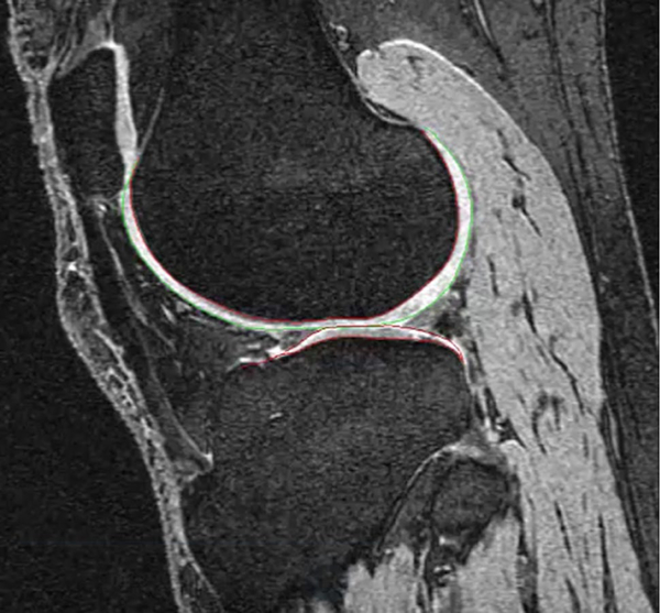
Tibia and femur automatic segmentation results on the 3D dual-echo steady state (DESS) sequence for the Osteoarthritis Initiative dataset obtained with active appearance modeling (Image credit: Mike Bowes, Imorphics, UK)

Despite promising results, the model-based nature of all algorithms built on the top of the SSM theory are characterized by a lack of local accuracy. Local shape features that are not correctly modeled in training, due to small sample sizes or high subject variability, are usually poorly addressed in the test set. For example, this class of techniques cannot properly identify the presence of osteophytes or severe cartilage loss. Thus, this method offers an optimal segmentation algorithm with a suboptimal performance in the extraction of imaging biomarkers, such as in late-stage OA progression where large shape variations are observed. In terms of computational time demands, the compact description of complex shapes with few principal components make the SSM-based methods a fast solution for the analysis of test data.

Atlas-based approaches

Atlas-based algorithms constitute another class of promising approaches. Overall, these strategies shift the post-processing focus from segmentation to registration. Image registration is the process of defining the best transformation to align two or more images. In atlas-based approaches, a reference is defined by a specific instance in the dataset or by merging N images previously aligned in a common coordinate system. For this atlas approach, a gold standard segmentation is manually conducted by an expert. Image registration applies this segmentation to the coordinate system of each case that needs to be segmented, typically applying an affine or non-rigid registration. However, it is well known that the manual gold-standard segmentation is subject to user variability, making image registration a difficult task to complete. Multi-atlas approaches attempt to manage this variability and minimize the registration error. The main strategy is based on constructing several atlases and registering all to the same target image. The final segmentation will be computed through label fusion methods.

Tamez-Pena et al. [37] presented a pilot study aimed at showing the feasibility of these techniques to segment articular cartilage. The study analyzed 19 subjects from the Osteoarthritis Initiative dataset. The segmentation was evaluated on 3D DESS images. The sequence settings included: pixel spacing (0.37 mm, 0.46 mm) slice thickness = 0.7 mm, TE/TR 4.7/16.3 mm. The CV of the automatic estimation of cartilage volume varied from 2.5 to 7.5 %, and thickness from 4.4 to 7.0 %.

Shan et al. [38, 39] recently proposed a multi-atlas strategy for both bone and cartilage segmentations, combined with a three-label approach that made use of the atlas segmentations as prior terms in a probabilistic approach. The method was evaluated on 706 images of the Pfizer Longi-tudinal Study [39]. This study extensively discussed the choice of different types of regularizers. They showed how anisotropic regularization could improve segmentation performances. Much of the study also focused on the choice of the classifier. K Nearest Neighbors (KNN) and Support Vector Machines (SVM) were tested. For the femoral cartilage, KNN and SVM showed similar performances, while the SVM outperformed the KNN on the tibial cartilage. The algorithm was also tested on the SKI10 dataset [33] showing competitive results: femur cartilage average Jaccard values were 75.3 and 75.6 % for femur and tibia, respectively.

Carbadillo-Gamio et al. [40] also presented an atlas approach for the analysis of thickness and T₂ relaxation times in patella cartilage. This method, compared to previously cited works, registered all the target images in the space of the atlas template, allowing for local statistical analysis. This method was recently modified and expanded on the overall knee joint [19].

The challenge of image registration makes the atlas-based segmentation techniques difficult to implement. The specific shape of the cartilage makes the interpolation step of transferring the segmentation mask from the atlas to the target image highly critical. Different choices in this phase may overestimate or underestimate the cartilage volume and thickness. Thus, algorithm setting should be always properly done, and comparison with a manually segmented gold standard should be considered. Mixing data from different pipelines should only be done after a proper cross sectional calibration of the results. Registration and label fusion, in the case of multi-atlas approaches, are both highly computational and intensive tasks, making the atlas-based methods unsuitable for real-time application. On the other hand, Shamonin et al. [41] showed how the usage of a GPU can sensitively speed up one of the most widely used state-of-the-art registration toolkit (elastix [42, 43]). This paper outlines how several of the non-rigid registration processing steps are highly parallelizable through Gaussian pyramids and the resampling step. The Gaussian filtering relies on a line-by-line causal and anti-causal filtering, where all image scan lines can be independently processed. The resampling step requires the same independent operation for every voxel. Moreover, the parallel implementation preserves the accuracy of the registration. These features make GPU an attractive tool capable of balancing segmentation time and result accuracy in non-rigid image registration, consistent with the application of atlas-based segmentation.

Graph-based approaches

Graph-based methods also play a big role in the knee segmentation literature. The s/t graph-cuts framework proposed by Boykov et al. [44] offers an object extraction method for N-dimensional images. Each voxel in the image is described as a node of a graph, where the weight of the graph’s edge connecting two nodes is related to both regional and boundary properties. There are several semiautomatic applications of this method. Shim et al. [45] showed how the use of the graph-cuts method significantly expedites the process of cartilage segmentation. Ababneh et al. [46] later proposed a fully automatic graph cut for bone segmentation. This method was evaluated on 376 MR images from the Osteoarthritis Initiative (OAI) database, and showed very high segmentation performances (0.95 Dice similarity index). Nevertheless, no experiments using similar techniques for cartilage segmentation are reported in this specific study.

Contrary to what was described for model-based and atlas-based methods, the graph-based technique does not model previous knowledge about the expected anatomy. This often results in better performances for extracting morphological biomarkers in late stages of disease. On the other hand, the lack of a model can also cause pitfalls in the algorithm. Systematic quality controls on segmentation results should always be considered in the pipeline if graph-based approaches are used for the segmentation. Graph-cut methods offer an approximate way to solve complex minimization problems [44] generally obtaining a good balancing between time and segmentation performance.

Machine learning-based approaches

In the last few years, a great deal of work has been done to employ machine learning (ML) techniques to solve medical imaging segmentation tasks [47]. Both unsupervised and supervised techniques have been proposed. In unsupervised strategies, the algorithm does not need any training dataset. Image labeling is completed by exploiting latent patterns in the voxel intensity distribution or other features and applying clustering techniques. On the other hand, supervised learning techniques require a training set so the algorithm can learn the correct label for each voxel through examples. Folkesson et al. [48, 49] presented a method based on the K nearest neighbor (KNN) classification strategy, and showed successful cartilage segmentation performances in the medial side of the joint on low-field MR images. A hierarchical schema was presented in this study. In the first step, cartilage was segmented from the background, which led to several false positives. This step was refined by a three-label classification strategy in the second step. A features vector was considered, taking the intensity of a single voxel and close neighbors into account. Parasoon et al. [50] further modified the work of Folkesson et al. by showing the combined use of KNN classifier and support vector machine (SVM). SVM is a widely used ML technique that shows promising results in solving different classification problems. The main obstacle is that SVM assumes that input data instances are independent and identically distributed (i.i.d.), which may not be appropriate for cartilage segmentation from MR images if single-voxel intensity is used as a feature for classification. Zhang et al. [51] proposed a strategy aimed to incorporate contextual information, such as normalized intensity, local image structures and geometrical features in a multi-contrast schema. One of the most interesting characteristics of machine learning-based approaches is the ability to build feature vectors composed of heterogeneous information, allowing for the simultaneous use of multiple images to solve the segmentation problem. In this specific work, T₁-weighted, FS SPGR, T₂/T₁-weighted fast imaging employing steady-state acquisition (FIESTA) and T₂/T₁-weighted iterative decomposition of water and fat with echo asymmetry and least-squares estimation (IDEAL)-gradient echo (GRE) water and fat images are simultaneously used to accomplish the cartilage segmentation task. The same group also previously presented a multi-contrast approach combined with a discriminative random field approach [52]. Despite the promising results from both of these studies, the testing sample size was relatively small (11 knees) and the algorithms were tested exclusively on healthy subjects. Pang et al. [53] recently proposed a method based on a pattern recognition approach by using gradient information for the knee articular cartilage segmentation, and reported a mean Dice coefficient equal to 0.76.

Generally, defining the best set of features for segmentation is a difficult task. Several attempts were made in the past to define a perfect features vector, which included intensity, texture, gradients, etc. Recently, the direction of ML research is to utilize the learning procedure to define a better transformation of raw data into a representation that can effectively accomplish the assigned task. Deep learning is a relatively new branch of ML, aimed at avoiding any a priori feature definitions and at better classifying patterns in the analyses of big datasets. To the best of our knowledge, to date, only one application of deep learning to solve the knee segmentation task has been published [54].

Due to the multitude of ML approaches, comparing the main features and results of each is a difficult task. However, it is worth mentioning the extreme importance of the training set, the proper number of training examples, and coverage of the possible data variability. An improperly balanced training set could create bias in the learning process of the machine, which could be translated into dangerous and inaccurate drifts of the measured biomarker.

In general for all the neural networks, but even more for the novel deep learning convolutional neural network, training is well known to be a highly intensive and computationally demanding process. On the other hand, training on big datasets has demonstrated how these techniques have overcome the most powerful state-of-the-art methods in solving extremely complex segmentation tasks [55, 56]. These applications clearly highlight how such a system with high performance can allow for proper training, exploiting the real power of the techniques. After the training phase, the application on the test set is generally a fast process, suitable for real-time application.

In this section, the four main classes of algorithms used to automatically solve knee segmentation were presented: model-based, atlas-based, graph-based and machine learning-based. Due to the complementary strengths and weaknesses of these methods, several attempts have been made to hybridize the approaches and combine strategies from different classes [57–61].

Hip cartilage segmentation

Several of the biomarkers used to assess knee cartilage, such as volume, thickness, and compositional imaging quantification, can also apply to hip cartilage. In assessment of hip MR images, perhaps the most interesting and difficult segmentation challenge is to automatically identify the femoral and acetabular cartilage borders. Compared with the knee joint, hip cartilage is much thinner, with an average thickness of 1.4 and 1.2 mm for the femoral and acetabular plates, respectively [62]. Moreover, due to the high curvature of the cartilage, the large majority of the voxels that compose the cartilage are severely affected by partial volume effect. The distinction between the individual cartilage plates (femoral and acetabular) is particularly challenging in weight-bearing areas without the use of leg traction devices or contrast agents [63, 64].

Semiautomatic edge-based methods

Semi-automatic methods have been proposed to accomplish hip cartilage segmentation, several of which employ edge-based algorithms. These strategies primarily use image gradient information mediated by feasibility constraints, such as smoothing or a priori knowledge about the expected shape of the structure to be segmented.

Naish et al. [65] proposed the use of livewire for segmenting hip articular cartilage, with the intention to study weight-bearing effects in asymptomatic young volunteers. Livewire is a commonly used method for interactive image segmentation. The image is described as a weighted graph where nodes represent the image pixels and the arcs between nodes represent the relationships between neighboring pixels. A weight is assigned to each connection, typically a function of the edge strength between two pixels. The user defines the first and last node of the boundary. A graph searching strategy, such as Dikstra or A* algorithm, is used to find the best path that connects the two user-defined ends points. A path is considered best if it minimizes the weight of the visited arcs. This technique was tested on the global femoral and acetabular cartilage of six volunteers imaged on a 1.5T Philips scanner using a T₂-weighted 3D gradient-echo sequence: pixel spacing (0.78 × 0.78 mm) slice thickness 1.6 mm. TR/ TE = 15.4/5.9 ms. This study reported a global CV in computing the global thickness equal to 2.5 %.

In 2008, Li et al. [66] proposed a possible solution for the distinct segmentation of the two hip cartilage plates. Segmentation was performed semi-automatically using active contour. In this technique, the segmentation was initialized by an edge manually estimated by the user. The final boundary for the object of interest was then identified through the optimization of an energy function, modeled as a force and defined by balancing the attraction of the image gradients and the meet of constraints on border features, such as smoothness. In this study, a 2-D multiple-echo data image combination (MEDIC) sequence was used for the hip cartilage segmentation with an in-plane spatial resolution of 0.5 × 0.5 mm and a slice thickness of 3 mm TR/TE 432/20 ms. Nine subjects were tested and retested, and the algorithm reported a global volume repeatability measure RMSCV% equal to 3.6 and 5.6 % for the femoral head and the acetabulum, respectively.

Also in 2008, Carballido-Gamio et al. [67] proposed the use of a technique previously used to semi-automatically segment knee cartilage in order to analyze cartilage thickness, volume, and relaxometry parameters, such as T_1ρ and T₂ in the hip [68]. The proposed strategy is based on edge detection and Bezier splines with spatial contrast, and edge enhancement based on anisotropic diffusion filtering. In this study, five healthy subjects were imaged twice to assess the reproducibility of the strategy. The femoral and acetabular cartilages were segmented in a single slice chosen by the user. The MRI sequence used in this study was a 3D water excitation spoiled gradient-echo (WE-SPGR) with an in-plane resolution of 0.312 × 0.312 mm and 1.5-mm slice thickness TE/TR of 8.2/16.3 ms. Scan/rescan reproducibility was reported equal to: CVs 2.19 and 3.50 % for the cartilage thickness and volume, respectively. T_1ρ and T₂ CVs were reported as 2.03 and 5.89 %, respectively.

The semiautomatic nature of these algorithms allows for achieving a high level of accuracy, comparable to manual segmentation. Furthermore, the execution times for these techniques are typically fast. However, the human interaction introduces inter-and intrauser variability. Careful user training and cross-calibration of different individuals should always be considered in the usage of these techniques, particularly in longitudinal studies.

Fully automatic hip cartilage segmentation

Most of the methods presented for accomplishing the fully automatic knee cartilage segmentation have the necessary features to translate well to hip segmentation, if correctly parameterized or trained. Siversson et al. [69] proposed a multi-atlas approach for the fully automatic segmentation of hip cartilage. The aim of this study was to assess morphological TrueFISP and biochemical dGEMRIC hip images in 15 symptomatic subjects with mild or no radiographic osteoarthritis. Specific attention was given to the choice of label fusion strategy, testing a more conventional majority voting technique versus a local map STAPLE method. The global performances were presented as a function of the number of the templates used in the multi-atlas approach. As expected, STAPLE generally outperformed the majority-voting rule. Interestingly, the segmentation performance showed a logarithmic trend varying with the number of atlas templates, thereby justifying the choice of a relatively small number of atlas templates in favor of better time performances.

Despite the good results generally achieved by this strategy, the major limitation of this method was that the algorithm was not applied on a single cartilage plate, but on the global hip cartilage. Figure 2 shows an example of a 3D thickness map automatically computed using this method.

Fig. 2.

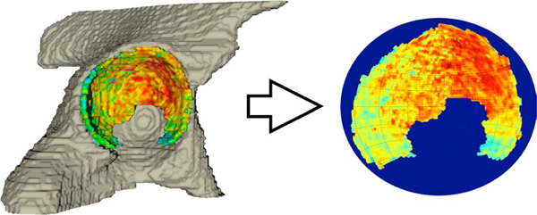
Example of thickness map automatically obtained with multi-atlas approach and STAPLE label fusion (Image courtesy credit: Carl Siversson, Ph.D., Computational Radiology Laboratory, Department of Radiology, Boston Children’s Hospital, Harvard Medical School, Boston, MA, USA; Department of Medical Radiation Physics, Lund University, Malmö, Sweden)

Xia et al. [63] proposed a combined use of ASM and graph-searching to solve automatic hipbone and cartilage segmentation. The proposed segmentation scheme included two phases: bone pre-segmentation and bone-cartilage interphase extraction, which was based on 3D ASM and a multilayer arc-weighted graph-based cartilage segmentation for the identification of the articular border and the division between the two cartilage plates. The main feature of this algorithm was that the femoral and acetabular cartilage plates were simultaneously segmented. Multiple surface feasibility constraints were considered in the graph construction (e.g., surface smoothness, inter-surface distance and inter-object separation). The goal of the method was to then co-optimize the inner and outer interfaces for both the femoral and acetabular cartilage plates. A training process on 26 manually segmented cases was used to extract local statistics on the cartilage morphology, such as the cartilage presence probability for each bone voxel, cartilage thickness (considering the mean, standard deviation, and ranges), and joint spacing, which was used to define the separation constraints. The difference in thickness between pairs of neighboring vertices was also computed from the training set and used as a smoothness constraint. The energy function designed for this model included a boundary term, smoothed prior penalty term, inter-surface prior penalty term and inter-object prior penalty term. The Bojkov Min-cut method was used to find the best surfaces. The algorithm demonstrated an excellent segmentation performance when tested on 52 healthy subjects. Automatic quantification of cartilage thickness and volume were highly correlated with manually derived values (R > 0.8), despite a general trend of overestimating the cartilage size.

Wrist segmentation

MRI evaluation of the wrist is particularly relevant in the study of RA. According to the Outcome Measures in Rheumatology Clinical Trials (OMERACT) MRI working group, which developed an MRI-based scoring system (RAMRIS), synovitis, bone marrow edema, and bone erosions are the three main signs of RA shown on MRI [70]. In particular, bone edemas and synovitis are abnormalities that precede irreversible joint destruction. Although shown to be sensitive and reproducible, RAMRIS is time consuming, thus making more quantitative assessments of the wrist joint highly desirable. From a technical point of view, analysis of the wrist is extremely challenging due to the small joint sizes and the many bones. Furthermore, the limited mobility and pain of RA patients make acquisition difficult, and motion artifacts often affect the MR images. To date, limited research has focused on developing automatic or semi-automatic procedures for wrist joint analysis.

Segmentation of the wrist bones

Koch et al. [71] proposed a strategy for the automatic segmentation of the single carpal bones. In this study, a random forest classifier was used to identify a bounding box for each bone. This detection phase was refined within an energy-based framework, and solved using a graph optimization strategy. This algorithm was evaluated on 59 T₁ weighted images and 51 T₂-weighted coronal MR images with a resolution of 0.365 × 0.365 in plane and 0.734 mm in slice thickness. The automatic results were compared with manually traced segmentations and the ROC Area Under the Curve (AUC) was reported for validation metrics. The performances achieved were 88.0 ± 10.6 % for the T data sets and 88.1 ± 9.2 % for the T₂ data sets. Unfortunately, this study does not report any information about the subjects analyzed. Moreover, it is not possible to assess the actual performance of the algorithm in correctly defining the bone border in the presence of erosion, synovitis or pannus tissue from these results.

Recently Wlodarczyk et al. [72] presented an atlas-based strategy for the wrist bone segmentation for low-field-strength MR images. The registration to the atlas was approached piecewise, dividing the problem into three sub-problems: registration of the distal parts of ulna and radius, the metacarpal bases, and the carpals. The authors reported that this choice was due to the computational demand of the algorithm, but also noted that this piecewise strategy helped to better control deformations in the registration phase. The atlas was only used in this strategy for the automatic definition of seeds used to automatically initialize a Watershed strategy, employed to finalize the segmentation. Excellent results were reported when the strategy was tested on 37 RA patients acquired on a 0.2 T MRI scanner. The average distance between the automatically and manually defined bone boundaries was approximately one pixel. Despite the good performance generally achieved, the authors acknowledged the lack of accuracy in segmenting big erosions with the proposed algorithm.

Bone marrow edema quantification

Bone marrow edema (BME) patterns are commonly seen in RA, corresponding to inflammation in subchondral bone and, possibly, angiogenesis. The MRI definition of BME is a region within trabecular bone demonstrating hyper intensity on T₂-weighted fat-suppressed images. Several studies have suggested BME as predictor of progression of erosion and joint damage in RA [73]. Li et al. [74, 75] proposed the use of a threshold-based method, previously adopted in the knee for the semiautomatic segmentation of BME in the wrists of patients with RA. In this study, 14 RA patients were analyzed, and images were acquired at 3T with an advanced water/fat separation fast spin-echo (FSE) sequence that used iterative decomposition of water and fat with echo asymmetry and least-squares estimation (IDEAL). This study showed how IDEAL sequences provide images with higher SNR than classical FSE. A better fat suppression in water images was also achieved using multi-frequency fat spectrum reconstruction.

For each case, the user traced five ROIs in the normal bone marrow regions to estimate the segmentation threshold, fixed at five times the standard deviation of the signal in the normal bone marrow ROIs. The user then traced another ROI, one that included the BME, and the threshold was applied. The technique repeatability was shown in the computation of the BME volume. Intra-observer ICC was reported to be 0.998 and RMS CV 2.3 %. The inter-observer ICC was 0.993 and RMS CV was 5.2 %, and the Scan/Rescan RMS-CV was 6.9 %. This method was then used for the analysis of perfusion parameters in the BMEL after multi-spectral registration. The same segmentation strategy was used in a subsequent study from the same group, aiming to assess the bone structure within the BME region using HR-pQCT [76]. Figure 3 shows an example of the segmentation results obtained by this technique in presence of big and small erosions (a1 and b1) and in absence of erosion (c1). The segmentation overlaid onto the HR-pQCT image after multimodal registration is also shown in Fig. 3a2, b2, and c2.

Fig. 3.

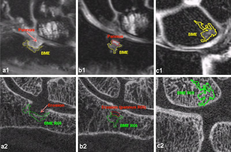
In the first row, an example is shown of bone marrow edema segmentation obtained with a semi-automatic threshold method applied on IDEAL FSE MRI imaging. The second row shows the segmented mask overlaid on the HR-pQCT after the application of multimodal registration (Image courtesy: Xiaojuan Li PhD, Department of Radiology and Biomedical Imaging, University of California, San Francisco, CA, USA)

The advantage of threshold-based methods is in the simple reproducibility of the technique between groups. On the other hand, results can be sensitive to MRI imaging settings, such as a fat suppression algorithm, which could lead to a systematic overestimation or underestimation of the BME volume. Caution should be used in mixing results coming from different protocols.

Conclusion

This paper covers automatic and semiautomatic techniques for joint and musculoskeletal tissue segmentation proposed in recent literature. A large body of work is available from the past decade, particularly for bone and cartilage segmentation in the knee and hip joints.

Table 1 summarizes the main classes of automatic segmentation techniques reviewed in this paper, highlighting the main strengths and drawbacks of each. Model- and atlas-based methods are the most widely used in the recent literature, and have been proven capable of obtaining the most successful results. However, with the growing availability of data, the increasing growth of computational power and data storage capability make machine learning approaches the most promising algorithm class for future applications, especially when applied in a multidimensional fashion and using information from different sequences.

Table 1.

Summary of algorithm classes frequently described in joint and musculoskeletal tissue segmentation

Algorithm class	Location of application	Main features	Strengths	Drawbacks
Model-based	Knee/hip	To define a model using a training set and to solve the target image segmentation by fitting the model	Robust because based on previous knowledge	Needs a relatively large training set Global modeling Robustness comes at the expense of lacking generalization from the training set
Atlas-based	Knee/hip/wrist	Manual segmentation of a reference image and Robust because based on previous knowl-registration of the segmented mask on the edge target image		Need of a efficient registration technique Results sensitive to the interpolation and label fusion technique chosen
Graph-based	Knee/hip	To describe the image features as a graph and translate the segmentation in an energy minimization problem	Flexible because not based on previous knowledge	Flexibility comes at the expense of lacking robustness Need of user initialization
Machine learning	Knee	Unsupervised: to learn statistical pattern from data	Robust because based on previous knowledge	Training is highly computationally demanding
		Supervised: to learn statistical pattern from training examples	Framework suitable for multispectral approaches	Needs a relatively large training set, when supervised
Semi automatic edge-based Knee/hip		To use information on the image gradients	Accuracy comparable with manual segmentation	Semiautomatic: need of user interaction
Semi automatic threshold-based	Wrist BME	To use information on the image Intensity	Easily reproducible results	Need of user interaction Sensitive to the imaging protocol and noise

For the knee, the presence of a standard benchmark dataset (MICCAI 2010 Workshop Medical Image Analysis for the Clinic—A Grand Challenge (SKI0)) allows for more accurate comparisons of different algorithms. Despite this large step towards a standardization of post-processing pipelines for knee bone and cartilage segmentation, there is still a lack of commonly accepted and widely distributed methods to solve this task. Too often, these methods remain a computer vision exercise; and in clinical studies, manual or semi-automatic segmentations are still more frequently used. In the analysis of the hip, more extensive validation of datasets with severely osteoarthritic subjects is required to make these techniques more widely available. Although some progress was made in the more quantitative and automatic analyses of the wrist joint in rheumatoid arthritis patients, several issues still need to be addressed, such as the automatic quantification of erosions (volume and shape), synovitis segmentation and quantification, as well as a more sophisticated fully automatic BME segmentation and quantification method.

In comparing different musculoskeletal anatomy, it is important to comment on the extensive use of SSM and atlas-based methods in spine segmentation, particularly for the analysis of lumbar and thoracic intervertebral discs (IVDs) and vertebral bodies (VBs) [77], and 3D segmentations of healthy and herniated intervertebral discs [78]. SSM was also recently used to identify the bone cartilage interface in the shoulder joint [79]. A combined use of SSM and atlas-based approaches has been presented in the segmentation of the quadratus lumborum muscle [80]. In 2015, Karlsson et al. [81] proposed a multi-atlas-based method used to quantify the whole-body skeletal muscle volume, and the volume of separate muscle groups. Figure 4 shows an example of automatic labeling of the different muscle groups obtained using this technique on a 3T scanner.

Fig. 4.

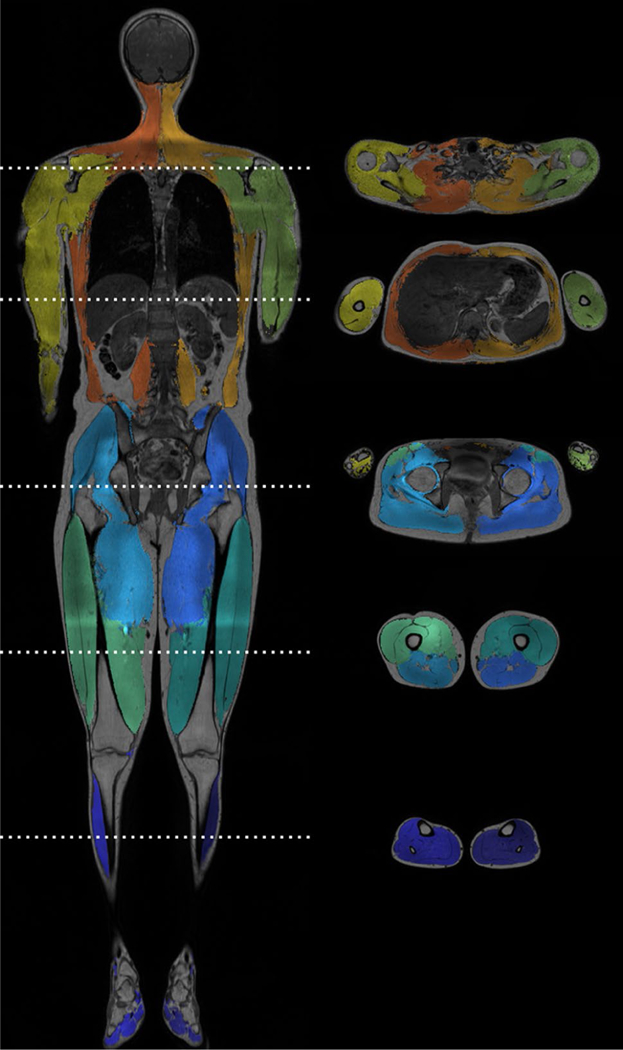
Example of automated muscle segmentation performed with a multi-atlas approach and applied on an image acquired at 3T (Image courtesy: Karlsson Anette, Department of Biomedical Engineering (IMT), Linköping University, Linköping, Sweden)

Although this review gives an overview on the classes of algorithms proposed for automatic segmentation of joint and musculoskeletal tissue in the last few years, several promising methods are not covered. Approaches widely used in neighboring research fields, such as neuroimaging, could be adapted for use in musculoskeletal applications [82]. The most recent computer vision and machine learning methods [83, 84], despite excellent performances shown in the segmentation of natural images, are still not widely translated in medical imaging field.

The automatic segmentation of joint and musculoskeletal tissues is still a major challenge for medical image processing. With the standardization in MRI acquisition and biomarker identification, automatic segmentation is an inevitable step in order to move from analyzing small datasets where manual segmentation is a feasible solution, to larger datasets and multicenter trials, obtaining more standardized and reliable measures. Moreover, several promising quantitative MRI analyses could have a much smoother translation into clinical practices if automatic segmentation can be achieved. Automatic joint and musculoskeletal tissue segmentation can be applied to new statistical analyses of “big data”, such as topological data analysis or deep learning latent pattern exploitation, which would help clinicians to better understand disease pathophysiology and disease phenotyping. A major multidisciplinary and collaborative effort is necessary from the entire musculoskeletal imaging community to collect public datasets, and manually create commonly accepted gold-standard segmentations and validation procedures. Researchers must expand from comparing quantification data between automatic and manual segmentations, begin to accurately translate segmentation performances of biomarker quantification, and relate these performances to the precision needed to detect, track, and predict disease progression.

References

- 1.The burden of musculoskeletal diseases 2009 Rosemont, IL, USA: usbjd.org. 2008. http://www.boneandjointburden.org
- 2.Woolf AD, Pfleger B (2003) Burden of major musculoskeletal conditions. Bull World Health Organ 81(9):646–656 [PMC free article] [PubMed] [Google Scholar]
- 3.Barbour KE, Helmick CG, Theis KA, Murphy LB, Hootman JM, Brady TJ, Cheng YJ (2013) Prevalence of doctor-diagnosed arthritis and arthritis-attributable activity limitation—United States, 2010–2012. Morb Mortal Wkly Rep 62(44):869–873 [PMC free article] [PubMed] [Google Scholar]
- 4.Hawamdeh Ziad M, Al-Ajlouni Jihad M (2013) The clinical pattern of knee osteoarthritis in Jordan: a hospital based study. Int J Med Sci 10(6):790–795 [DOI] [PMC free article] [PubMed] [Google Scholar]
- 5.Lohmander L, Englund P, Dahl L, Roos E (2007) The long term consequence of anterior cruciate ligament and meniscus injuries: Osteoarthritis. Am J Sports Med 35(10):1756–1769 [DOI] [PubMed] [Google Scholar]
- 6.Helmick CG, Felson DT, Lawrence RC, Gabriel S, Hirsch R, Kwoh CK, Liang MH, Kremers HM, Mayes MD, Merkel PA, Pillemer SR, Reveille JD, Stone JH, National Arthritis Data Workgroup (2008) Estimates of the prevalence of arthritis and other rheumatic conditions in the United States. Part I. Arthritis Rheum 58(1):15–25 [DOI] [PubMed] [Google Scholar]
- 7.Wright NC, Looker AC, Saag KG, Curtis JR, Delzell ES, Randall S, Dawson-Hughes B (2014) The recent prevalence of osteoporosis and low bone mass in the United States based on bone mineral density at the femoral neck or lumbar spine. J Bone Miner Res 29(11):2520–2526 [DOI] [PMC free article] [PubMed] [Google Scholar]
- 8.Menashe L, Hirko K, Losina E, Kloppenburg M, Zhang W, Li L, Hunter DJ (2012) The diagnostic performance of MRI in osteo arthritis: A systematic review and meta-analysis. Osteoarthritis Cartilage 20(1):13–21 [DOI] [PMC free article] [PubMed] [Google Scholar]
- 9.McQueen F, Stewart N, Crabbe J, Robinson E, Yeoman S, Tan P, McLean L (1999) Magnetic resonance imaging of the wrist in early rheumatoid arthritis reveals progression of erosions despite clinical improvement. Ann Rheum Dis 58(3):156–163 [DOI] [PMC free article] [PubMed] [Google Scholar]
- 10.McQueen F, Benton N, Perry D, Crabbe J, Robinson E, Yeoman S, McLean L, Stewart N (2003) Bone edema scored on magnetic resonance imaging scans of the dominant carpus at presentation predicts radiographic joint damage of the hands and feet 6 years later in patients with rheumatoid arthritis. Arthritis Rheum 48(7):1814–1827 [DOI] [PubMed] [Google Scholar]
- 11.Hetland M, Ejbjerg B, Horslev-Petersen K, Jacobsen S, Vestergaard A, Jurik A, Stengaard-Pedersen K, Junker P, Lottenburger T, Hansen I, Andersen L, Tarp U, Skjødt H, Pedersen J, Majgaard O, Svendsen A, Ellingsen T, Lindegaard H, Christensen A, Vallø J, Torfing T, Narvestad E, Thomsen H, Ostergaard M (2008) MRI bone oedema is the strongest predictor of subsequent radio graphic progression in early rheumatoid arthritis. Results from a 2 yeas randomized controlled trial (CIMESTRA). Ann Rheum Dis 67(7):998–1003 [DOI] [PubMed] [Google Scholar]
- 12.Link Thomas M (2012) Osteoporosis imaging: State of the art and advanced imaging. Radiology 263(1):3–17 [DOI] [PMC free article] [PubMed] [Google Scholar]
- 13.Gonzalez RC, Woods RE (2001) Digital image processing, 2nd edn Addison-Wesley, Boston [Google Scholar]
- 14.Weckbach S, Mendlik T, Horger W, Wagner S, Reiser MF, Glaser C (2006) Quantitative assessment of patellar cartilage volume and thickness at 3.0 tesla comparing a 3D-fast low angle shot versus a 3D-true fast imaging with steady-state precession sequence for reproducibility. Invest Radiol 41(2):189–197 [DOI] [PubMed] [Google Scholar]
- 15.Eckstein F, Kunz M, Schutzer M, Hudelmaier M, Jackson RD, Yu J, Eaton CB, Schneider E (2007) Two year longitudinal change and test-retest-precision of knee cartilage morphology in a pilot study for the osteoarthritis initiative. Osteoarthritis Cartilage 15(11):1326–1332 [DOI] [PMC free article] [PubMed] [Google Scholar]
- 16.Schneider E, Nevitt M, McCulloch C, Cicuttini FM, Duryea J, Eckstein F, Tamez-Pena J (2012) Equivalence and precision of knee cartilage morphometry between different segmentation teams, cartilage regions, and MR acquisitions. Osteoarthritis Cartilage 20(8):869–879 [DOI] [PMC free article] [PubMed] [Google Scholar]
- 17.Jordan CD, McWalter EJ, Monu UD, Watkins RD, Chen W, Bangerter NK, Hargreaves BA, Gold GE (2014) Variability of CubeQuant T1ρ, quantitative DESS T2, and cones sodium MRI in knee cartilage. Osteoarthritis Cartilage 22(10):1559–1567 [DOI] [PMC free article] [PubMed] [Google Scholar]
- 18.Li X, Pedoia V, Kumar D, Rivoire J, Wyatt C, Lansdown D, Amano K, Okazaki N, Savic D, Koff MF, Felmlee J, Williams SL, Majumdar S (2015) Cartilage T1ρ and T2 relaxation times: Longitudinal reproducibility and variations using different coils, MR systems and sites. Osteoarthritis Cartilage 23(12):2214–2223 [DOI] [PMC free article] [PubMed] [Google Scholar]
- 19.Pedoia V, Li X, Su F, Calixto N, Majumdar S (2015) Fully automatic analysis of the knee articular cartilage T1ρ relaxation time using voxel-based relaxometry. J Magn Reson Imaging (Epub ahead of print) [DOI] [PMC free article] [PubMed] [Google Scholar]
- 20.Eckstein F, Kwoh CK, Boudreau RM, Wang Z, Hannon MJ, Cotofana S, Hudelmaier MI, Wirth W, Guermazi A, Nevitt MC, John MR, Hunter DJ, OAI investigators (2013) Quantitative MRI measures of cartilage predict knee replacement: A case-control study from the Osteoarthritis Initiative. Ann Rheum Dis 72(5):707–714 [DOI] [PubMed] [Google Scholar]
- 21.Neogi Tuhina, Bowes Michael A, Niu Jingbo, De Souza Kevin M, Vincent Graham R, Goggins Joyce, Zhang Yuqing, Felson David T (2013) Magnetic resonance imaging-based three-dimensional bone shape of the knee predicts onset of knee osteoarthritis. Arthritis Rheum 68(8):2048–2058 [DOI] [PMC free article] [PubMed] [Google Scholar]
- 22.Pedoia V, Lansdown DA, Zaid M, McCulloch CE, Souza R, Ma CB, Li X (2015) Three-dimensional MRI-based statistical shape model and application to a cohort of knees with acute ACL injury. Osteoarthritis Cartilage 23(10):1695–1703 [DOI] [PMC free article] [PubMed] [Google Scholar]
- 23.Lansdown DA, Zaid M, Pedoia V, Subburaj K, Souza R, Benjamin C, Li X (2014) Reproducibility measurements of three methods for calculating in vivo MR-based knee kinematics. J Magn Reson Imaging 42(2):533–538 [DOI] [PMC free article] [PubMed] [Google Scholar]
- 24.Zaid M, Lansdown D, Su F, Pedoia V, Tufts L, Rizzo S, Souza RB, Li X, Ma CB (2015) Abnormal tibial position is correlated to early degenerative changes 1 year following ACL reconstruction. J Orthop Res 33(7):1079–1086 [DOI] [PMC free article] [PubMed] [Google Scholar]
- 25.Lohmander L, Ionescu M, Jugessur H, Poole A (1999) Changes in joint cartilage aggrecan after knee injury and in osteoarthritis. Arthritis Rheum 42:534–544 [DOI] [PubMed] [Google Scholar]
- 26.Price J, Till S, Bickerstaff D, Bayliss M, Hollander A (1999) Degradation of cartilage type II collagen precedes the onset of osteoarthritis following anterior cruciate ligament rupture. Arthritis Rheum 42:2390–2398 [DOI] [PubMed] [Google Scholar]
- 27.Dunn TC, Lu Y, Jin H, Ries MD, Majumdar S (2004) T2 relaxation time of cartilage at MR imaging: Comparison with severity of knee osteoarthritis. Radiology 232:592–598 [DOI] [PMC free article] [PubMed] [Google Scholar]
- 28.Li X, Ma C, Link T et al. (2007) In vivo T1ρ and T2 mapping of articular cartilage in osteoarthritis of the knee using 3 Tesla MRI. Osteoarthritis Cartilage 15(7):789–797 [DOI] [PMC free article] [PubMed] [Google Scholar]
- 29.Cootes TF, Taylor CJ, Cooper DH, Graham J (1995) Active shape models-their training and application. Comput Vis Image Underst 1995(61):38–59 [Google Scholar]
- 30.Cootes TF, Edwards GJ, Taylor CJ (2001) Active appearance models. IEEE Trans Pattern Anal Mach Intell 23(6):681–685 [Google Scholar]
- 31.Solloway S, Hutchinson CE, Waterton JC, Taylor CJ (1997) The use of active shape models for making thickness measurements of articular cartilage from MR images. Magn Reson Med 37(6):943–952 [DOI] [PubMed] [Google Scholar]
- 32.Seim H, Kainmueller D, Lamecker H, Bindernagel M, Malinowski J, Zachow S (2010) Model-based Auto-Segmentation of Knee Bones and Cartilage in MRI Data MICCAI 2010 Workshop Medical Image Analysis for the Clinic—A Grand Challenge (SKI0) pp 215–223 [Google Scholar]
- 33.Heimann T, Morrison BJ, Styner MA, Niethammer M, Warfield SK (2010) Segmentation of Knee Images: A Grand Challenge www.ski10.org
- 34.Vincent G, Wolstenholme C, Scott I, Bowes M (2011) Fully Automatic Segmentation of the Knee Joint using Active Appearance Models Data MICCAI 2010 Workshop Medical Image Analysis for the Clinic—A Grand Challenge (SKI0) [Google Scholar]
- 35.Williams TG, Vincent G, Bowes M, Cootes T, Balamoody S, Hutchinson C, Waterton JC, Taylor CJ (2010) Automatic segmentation of bones and inter-image anatomical correspondence by volumetric statistical modelling of knee MRI. Biomedical Imaging: From Nano to Macro, 2010 IEEE International Symposium on, pp 432–435 [Google Scholar]
- 36.Williams TG, Holmes AP, Waterton JC, Maciewicz RA, Hutchinson CE, Moots Nash RJ, Taylor CJ (2010) Anatomically corresponded regional analysis of cartilage in asymptomatic and osteoarthritic knees by statistical shape modelling of the bone. IEEE Trans Med Imag 29(8):1541–1559 [DOI] [PubMed] [Google Scholar]
- 37.Tamez-Pena J, Gonzalez J, Farber J, Baum K, Schreyer E, Toter-man S (2011) Atlas based method for the automated segmentation and quantification of knee features: Data from the osteoarthritis initiative, in Proceeding IEEE International Symposium Biomedical Imaging pp 1484–1487 [Google Scholar]
- 38.Shan L, Charles C, Niethammer M (2012) Automatic multiatlas-based cartilage segmentation from knee MR images, Biomedical Imaging (ISBI), 2012 9th IEEE International Symposium on, pp 1028–1031 [DOI] [PMC free article] [PubMed] [Google Scholar]
- 39.Shan L, Zach C, Charles C, Niethammer M (2014) Automatic atlas-based three-label cartilage segmentation from MR knee images. Med Image Anal 18(7):1233–1246 [DOI] [PMC free article] [PubMed] [Google Scholar]
- 40.Carballido-Gamio J, Majumdar S (2011) Atlas-based knee cartilage assessment. Magn Reson Med 66(2):574–583 [DOI] [PMC free article] [PubMed] [Google Scholar]
- 41.Shamonin DP, Bron EE, Lelieveldt BPF, Smith M, Klain S, Starting M, Alzheimer’s Desease Neuroimeging Initiative (2014) Fast parallel image registration on CPU and GPU for diagnostic classification of Alzheimer’s disease. Front Neuroinform. doi: 10.3389/fninf.2013.00050 [DOI] [PMC free article] [PubMed] [Google Scholar]
- 42.Klein S, Staring M, Murphy K, Viergever MA, Pluim JPW (2010) Elastix: A toolbox for intensity-based medical image registration. IEEE Trans Med Imaging 29:196–205 [DOI] [PubMed] [Google Scholar]
- 43.Glocker B, Sotiras A, Komodakis N, Paragios N (2011) Deformable medical image registration: Setting the state of the art with discrete methods. Annu Rev Biomed Eng 15(13):219–244 [DOI] [PubMed] [Google Scholar]
- 44.Boykov Y, Veksler O (2001) Fast approximate energy minimization via graph cuts. IEEE Trans Pattern Anal Mach Intell 23(11):1222–1239 [Google Scholar]
- 45.Shim H, Chang S, Tao C, Wang JH, Kwoh CK, Bae KT (2009) Knee cartilage: Efficient and reproducible segmentation on high-spatial-resolution MR images with the semiautomated graph-cut algorithm method. Radiology 251(2):548–556 [DOI] [PubMed] [Google Scholar]
- 46.Ababneh SY, Prescott JW, Gurcan MN (2011) Automatic graph-cut based segmentation of bones from knee magnetic resonance images for osteoarthritis research. Med Image Anal 15(4):438–448 [DOI] [PMC free article] [PubMed] [Google Scholar]
- 47.Jain V, Seung HS, Turaga SC (2010) Machines that learn to segment images: A crucial technology for connectomics. Curr Opin Neurobiol 20(5):653–666 [DOI] [PMC free article] [PubMed] [Google Scholar]
- 48.Folkesson J, Dam E, Olsen OF, Pettersen P, Christiansen C (2005) Automatic segmentation of the articular cartilage in knee MRI using a hierarchical multi-class classification scheme. Med Image Comput Comput Assist Interv 8(Pt 1):327–334 [DOI] [PubMed] [Google Scholar]
- 49.Folkesson J, Dam EB, Olsen OF, Pettersen PC, Christiansen C (2007) Segmenting articular cartilage automatically using a voxel classification approach. IEEE Trans Med Imaging 26(1):106–115 [DOI] [PubMed] [Google Scholar]
- 50.Prasoon A, Igel C, Loog M, Lauze F, Dam EB, Nielsen M (2013) Femoral cartilage segmentation in Knee MRI scans using two stage voxel classification, Engineering in Medicine and Biology Society (EMBC), 35th Annual International Conference of the IEEE, pp 5469–5472 [DOI] [PubMed] [Google Scholar]
- 51.Zhang K, Lu W, Marziliano P (2013) Automatic knee cartilage segmentation from multi-contrast MR images using support vector machine classification with spatial dependencies. Magn Reson Imaging 31(10):1731–1743 [DOI] [PubMed] [Google Scholar]
- 52.Zhang K, Lu W (2011) Automatic human knee cartilage segmentation from multi-contrast MR images using extreme learning machines and discriminative random fields. In Proceedings of the Second international conference on Machine learning in medical imaging, pp 335–343 [Google Scholar]
- 53.Pang J, Li P, Qiu M, Chen W, Qiao L (2015) Automatic articular cartilage segmentation based on pattern recognition from knee MRI images. J Digit Imaging (Epub ahead of print) [DOI] [PMC free article] [PubMed] [Google Scholar]
- 54.Prasoon A, Petersen K, Igel C, Lauze F, Dam E, Nielsen M (2013) Deep feature learning for knee cartilage segmentation using a triplanar convolutional neural network. Med Image Comput Comput Assist Interv 16:246–253 [DOI] [PubMed] [Google Scholar]
- 55.Ciresan DC, Giusti A, Gambardella LM, Schmidhuber J (2013) Mitosis detection in breast cancer histology images with deep neural networks. Med Image Comput Comput Assist Interv 16:411–418 [DOI] [PubMed] [Google Scholar]
- 56.Cires C, Gambardella L, Schmidhuber J (2012) Deep neural networks segment neuronal membranes in electron microscopy images NIPS: Twenty-sixth Conference on Neural Information Processing Systems; Harrahs and Harveys, Lake Tahoe, pp 2852–2860 [Google Scholar]
- 57.Yin Y, Williams R, Anderson DD, Sonka M (2010) Hierarchical Decision Framework with a Priori Shape Models for Knee Joint Cartilage Segmentation MICCAI 2010 Workshop Medical Image Analysis for the Clinic—A Grand Challenge (SKI0) pp 241–250 [Google Scholar]
- 58.Lee S, Park SH, Shim H, Yun D, Lee S (2011) Optimization of local shape and appearance probabilities for segmentation of knee cartilage in 3-D MR images. Comput Vis Image Underst 115(12):1710–1720 [Google Scholar]
- 59.Wang Z, Donoghue C, Rueckert D (2013) Patch-based segmentation without registration: Application to knee MRI lecture notes in computer science machine learning in medical. Imaging 8184(2013):98–105 [Google Scholar]
- 60.Lee JG, Gumus S, Moon CH, Kwoh CK, Bae KT (2014) Fully automated segmentation of cartilage from the MR images of knee using a multi-atlas and local structural analysis method. Med Phys 41(9):092303. [DOI] [PMC free article] [PubMed] [Google Scholar]
- 61.Wang Q, Wu D, Lu L, Liu M, Boyer KL, Zhou SK (2014) Semantic Context Forests for Learning-Based Knee Cartilage Segmentation in 3D MR Images. Medical Computer Vision Large Data in Medical Imaging Lecture Notes in Computer Science, vol 8331 Springer, Newyork, pp 105–115 [Google Scholar]
- 62.Xia Y, Chandra SS, Engstrom C, Strudwick MW, Crozier S, Fripp J (2014) Automatic hip cartilage segmentation from 3D MR images using arc-weighted graph searching. Phys Med Biol 59(23):7245–7266 [DOI] [PubMed] [Google Scholar]
- 63.Cheng Y, Guo C, Wang Y, Bai J, Tamura S (2013) Accuracy limits for the thickness measurement of the hip joint cartilage in 3D MR images: Simulation and validation. IEEE Trans Biomed Eng 60(2):517–533 [DOI] [PubMed] [Google Scholar]
- 64.Baniasadipour A, Zoroofi RA, Sato Y, Nishii T, Nakanishi K, Tanaka H, Sugano N, Yoshikawa H, Nakamura H, Tamura S (2007) A fully automated method for segmentation and thickness map estimation of femoral and acetabular cartilages in 3D CT images of the hip 5th International Symposium on Image and Signal Processing and Analysis, pp 92–97 [Google Scholar]
- 65.Naish JH, Xanthopoulos E, Hutchinson CE, Waterton JC, Taylor CJ (2006) MR measurement of articular cartilage thickness distribution in the hip. Osteoarthritis Cartilage 14:967–973 [DOI] [PubMed] [Google Scholar]
- 66.Li W, Abram F, Beaudoin G, Berthiaume M-J, Pelletier J- P, Martel-Pelletier J (2008) Human hip joint cartilage: MRI quantitative thickness and volume measurements discriminating acetabulum and femoral head. IEEE Trans Biomed Eng 55(12):2731–2740 [DOI] [PubMed] [Google Scholar]
- 67.Carballido-Gamio J, Link TM, Li X, Han ET, Krug R, Ries MD, Majumdar S (2008) Feasibility and reproducibility of relaxometry, morphometric, and geometrical measurements of 76. the hip joint with magnetic resonance imaging at 3T. J Magn Reson Imaging 28:227–235 [DOI] [PubMed] [Google Scholar]
- 68.Carballido-Gamio J, Bauer JS, Stahl R et al. (2008) Inter-subject comparison of MRI knee cartilage thickness. Med Image Anal 12(2):120–135 [DOI] [PMC free article] [PubMed] [Google Scholar]
- 69.Siversson C, Akhondi-Asl A, Bixby S, Kim YJ, Warfield SK Three-dimensional hip cartilage quality assessment of morphology and dGEMRIC by planar maps and automated segmentation. Osteoarthritis Cartilage 22(10):1511–1515. [DOI] [PMC free article] [PubMed] [Google Scholar]
- 70.Ostergaard M, Peterfy C, Conaghan P, McQueen F, Bird P, Ejb-jerg B, Shnier R, O’Connor P, Klarlund M, Emery P, Genant H, Lassere M, Edmonds J (2003) OMERACT rheumatoid arthritis magnetic resonance imaging studies. Core set of MRI acquisitions, joint pathology definitions, and the OMERACT RA-MRI scoring system. J Rheumatol 30(6):1385–1386 [PubMed] [Google Scholar]
- 71.Koch M, Schwing AG, Comaniciu D, Pollefeys M (2011) Fully automatic segmentation of wrist bones for arthritis patients, Biomedical Imaging: From Nano to Macro, IEEE International 80. Symposium on, pp 636–640 [Google Scholar]
- 72.Wlodarczyk J, Czaplicka K, Tabor Z, Wojciechowski W, Urbanik A (2015) Segmentation of bones in magnetic resonance images of the wrist. Int J Comput Assist Radiol 10(4):419–431.. [DOI] [PMC free article] [PubMed] [Google Scholar]
- 73.Hetland ML, Stengaard-Pedersen K, Junker P et al. (2010) Radiographic progression and remission rates in early rheumatoid arthritis MRI bone oedema and anti-CCP predicted radiographic progressionin the 5-year extension of the double-blind randomized CIMESTRA trial. Ann Rheum Dis 69:1789–1795. [DOI] [PubMed] [Google Scholar]
- 74.Li X, Ma C, Bolbos R, Stahl R, Lozano J, Zuo J, Lin K, Link T, Safran M, Majumdar S (2008) Quantitative assessment of bone marrow edema pattern and overlying cartilage in knees with osteoarthritis and anterior cruciate ligament tear using MR imaging and spectroscopic imaging. J Magn Reson Imaging 28(2):453–461. [DOI] [PMC free article] [PubMed] [Google Scholar]
- 75.Li X, Yu A, Virayavanich W, Noworolski SM, Link TM, Imboden J (2012) Quantitative characterization of bone marrow edema pattern in rheumatoid arthritis using 3 Tesla MRI. J Magn Reson Imaging 35(1):211–218 [DOI] [PubMed] [Google Scholar]
- 76.Teruel JR, Burghardt AJ, Rivoire J, Srikhum W, Noworolski SM, Link TM, Imboden JB, Li X (2014) Bone structure and perfusion quantification of bone marrow edema pattern in the wrist of patients with rheumatoid arthritis: A multimodality study. J Rheumatol 41(9):1766–1773 [DOI] [PubMed] [Google Scholar]
- 77.Neubert A, Fripp J, Engstrom C, Schwarz R, Lauer L, Salvado O, Crozier S (2012) Automated detection, 3D segmentation and analysis of high resolution spine MR images using statistical shape models. Phys Med Biol 57(24):8357–8376 [DOI] [PubMed] [Google Scholar]
- 78.Haq R, Aras R, Besachio DA, Borgie RC, Audette MA (2015) 3D lumbar spine intervertebral disc segmentation and compression simulation from MRI using shape-aware models. Int J Com-put Assist Radiol Surg 10(1):45–54 [DOI] [PubMed] [Google Scholar]
- 79.Yang Z, Fripp J, Chandra SS, Neubert A, Xia Y, Strudwick M, Paproki A, Engstrom C, Crozier S (2015) Automatic bone segmentation and bone-cartilage interface extraction for the shoulder joint from magnetic resonance images. Phys Med Biol 60(4):1441–1459 [DOI] [PubMed] [Google Scholar]
- 80.Engstrom CM, Fripp J, Jurcak V, Walker DG, Salvado O, Crozier S (2011) Segmentation of the quadratus lumborum muscle using statistical shape modeling. J Magn Reson Imaging 33(6):1422–1429 [DOI] [PubMed] [Google Scholar]
- 81.Karlsson A, Rosander J, Romu T, Tallberg J, Gronqvist A, Borga M, Dahlqvist Leinhard O (2015) Automatic and quantitative assessment of regional muscle volume by multi-atlas segmentation using whole-body water-fat MRI. J Magn Reson Imaging 41(6):1558–1569 [DOI] [PubMed] [Google Scholar]
- 82.Gordillo N, Montseney E, Sobervilla P et al. (2013) State of the art survey on MRI brain tumor segmentation. Magn Reson Imaging 31(8):1426–1438 [DOI] [PubMed] [Google Scholar]
- 83.Li Z, Chen J (2015) Superpixel Segmentation Using Linear Spectral Clustering, The IEEE Conference on Computer Vision and Pattern Recognition (CVPR) in press [Google Scholar]
- 84.Long J, Shelhamer E, Darrell T (2015) Fully Convolutional Networks for Semantic Segmentation The IEEE Conference on Computer Vision and Pattern Recognition (CVPR) in press [DOI] [PubMed] [Google Scholar]