Axial changes in wood functional traits have limited net effects on stem biomass increment in European beech (Fagus sylvatica)

Abstract

During the growing season, trees allocate photoassimilates to increase their aboveground woody biomass in the stem (ABI_stem). This ‘carbon allocation’ to structural growth is a dynamic process influenced by internal and external (e.g., climatic) drivers. While radial variability in wood formation and its resulting structure have been intensively studied, their variability along tree stems and subsequent impacts on ABI_stem remain poorly understood. We collected wood cores from mature trees within a fixed plot in a well-studied temperate Fagus sylvatica L. forest. For a subset of trees, we performed regular interval sampling along the stem to elucidate axial variability in ring width (RW) and wood density (ρ), and the resulting effects on tree- and plot-level ABI_stem. Moreover, we measured wood anatomical traits to understand the anatomical basis of ρ and the coupling between changes in RW and ρ during drought. We found no significant axial variability in ρ because an increase in the vessel-to-fiber ratio with smaller RW compensated for vessel tapering towards the apex. By contrast, temporal variability in RW varied significantly along the stem axis, depending on the growing conditions. Drought caused a more severe growth decrease, and wetter summers caused a disproportionate growth increase at the stem base compared with the top. Discarding this axial variability resulted in a significant overestimation of tree-level ABI_stem in wetter and cooler summers, but this bias was reduced to ~2% when scaling ABI_stem to the plot level. These results suggest that F. sylvatica prioritizes structural carbon sinks close to the canopy when conditions are unfavorable. The different axial variability in RW and ρ thereby indicates some independence of the processes that drive volume growth and wood structure along the stem. This refines our knowledge of carbon allocation dynamics in temperate diffuse-porous species and contributes to reducing uncertainties in determining forest carbon fixation.

Introduction

Plants dominate the global biomass within the biosphere (Bar-On et al. 2018), with forests being particularly effective in sequestering and storing atmospheric carbon (Pan et al. 2011, Le Quéré et al. 2018). This ecosystem property has fuelled interest in studying carbon allocation in trees — i.e., the partitioning of photosynthates between different above- and belowground sink tissues (foliage, stem, coarse and fine roots), nonstructural carbohydrate pools, root exudates and maintenance respiration (Litton et al. 2007, Luyssaert et al. 2007, Dietze et al. 2014). It has been shown that this partitioning of resources can change as a function of climate, atmospheric CO₂ concentration and nutrient availability (Chen et al. 2013, Lapenis et al. 2013, Mcmurtrie and Dewar 2013, Mausolf et al. 2019). This impacts the carbon storage capacity of forests, which increases (decreases) with higher (lower) carbon investment in long-term pools such as the stem (Körner 2017). Accordingly, considerable efforts have been invested in quantifying temporal variability and trends in aboveground woody biomass increment (Babst et al. 2014a) and in mechanistic modeling of carbon allocation to stem growth (Li et al. 2014, Gea-Izquierdo et al. 2015, Guillemot et al. 2017, He et al. 2019). Still, our understanding of — and thus our ability to mathematically describe — the relevant processes that govern carbon source activity in trees remains much more advanced compared with our knowledge of carbon sink activities and their external and internal drivers (Zuidema et al. 2018, Fatichi et al. 2019). Consequently, a current research priority is to better understand wood formation processes and their environmental constraints in trees (e.g., Castagneri et al. 2015, von Arx et al. 2017, Cuny et al. 2019), which should then be translated into refined mechanistic model structures that balance source and sink constraints on tree growth.

In their recent article, Friend et al. (2019) proposed an interesting concept to implement wood formation in dynamic global vegetation models as individual wood cells that go through the different developmental stages (Rathgeber et al. 2016) and are influenced by internal and external drivers. Similar to most existing field studies of tree growth (e.g., Klesse et al. 2018), this approach relies on the assumption that wood formation at one location along the stem is representative of the dynamics of volume and mass growth for the entire stem. However, while wood formation in higher stem sections has rarely been assessed, some studies have provided evidence for axial changes in the climate sensitivity of radial growth. For example, Bouriaud et al. (2015) and van der Maaten and Bouriaud (2012) measured radial growth and wood density (ρ) at multiple positions along the stem of Picea abies and Abies alba trees in temperate Europe and found a decrease in climate sensitivity towards higher stem sections. By contrast, Kerhoulas and Kane (2012) reported higher climate sensitivity at the top compared with the bottom of the stem in Pinus ponderosa from Arizona. They attributed this pattern to hydraulic limitations under drought and also indicated a prioritization of carbon allocation to root growth when climatic conditions were unfavorable. Chhin et al. (2010) studied almost 400 Pinus contorta trees from western Canada and discovered a relatively complex seasonality of previous and current year climatic influences on growth at different stem heights. Taken together, these studies have left us with a somewhat unclear picture of axial growth variability that needs to be clarified to support the realistic implementation of carbon sink activity in mechanistic vegetation models (Zuidema et al. 2018, Fatichi et al. 2019). Doing so requires establishing a quantitative link between wood functional traits and the aboveground woody biomass increment in the stem (ABI_stem) of mature trees, which has rarely been achieved.

Novel studies on xylem characteristics have provided key insights in wood functional traits and their response to environmental variability (Castagneri et al. 2015, Arx et al. 2017, Björklund et al. 2017, Cuny et al. 2019). Despite these recent advances, it remains unclear how wood density is impacted by axial changes in cell parameters such as diameter, lumen area or wall thickness. Current understanding of xylogenesis is that wood cell production and elongation (which drive radial growth and wood density) are influenced internally by the turgor pressure within the cambium, by hormones and by the concentration of nonstructural carbohydrates in the phloem (De Schepper and Steppe 2010, Hartmann et al. 2017). These mechanisms are controlled by gradients originating from the tree’s apex (e.g., Woodruff et al. 2004, Rathgeber et al. 2011). At the same time, the diameter of wood cells universally tapers towards the apex (West et al. 1999, Anfodillo et al. 2006, Olson et al. 2014, Williams et al. 2019) to mitigate the dropping stem water potential with increasing tree height. Without simultaneous changes in cell wall area, the result will be an increase in the ratio between cell wall to lumen area, which should cause an increase in wood density from the stem base towards the apex (Hypothesis 1, tested in this study; H1). Together, these processes suggest that carbon allocation to wood formation in tree stems should vary as a function of distance from the apex, but this pattern has seldom been quantified in terms of actual biomass increment.

It has been shown that trees can prioritize carbon allocation to belowground sinks under unfavorable environmental conditions (Kerhoulas and Kane 2012, Lapenis et al. 2013). In addition, the tree may favor carbon sinks that are proximal to the source (i.e., the canopy) when resources are limiting, regulated by axial gradients in hormones and phloem sugar concentration (e.g., Rathgeber et al. 2011). If this is the case, radial growth should be tempered more strongly in lower compared with upper stem parts under suboptimal climatic conditions (Hypothesis 2; H2). Some evidence for this comes from the occurrence of so-called ‘missing rings’ in tree-ring records, i.e., when no ring is formed at sampling height in a particularly cold and/or dry year (Fritts et al. 1965, Wilmking et al. 2012). In light of possible axial changes in carbon allocation to the stem, van der Maaten and Bouriaud (2012) stated that the ubiquitous measurements of radial growth at breast height could give a biased representation of aboveground volume and biomass increment. Indeed, if breast height measurements were to underestimate growth in unfavorable years, the fraction of the sequestered carbon that is invested in ABI_stem could be larger than previously reported (Hypothesis 3; H3). A careful evaluation of this potential bias is warranted because tree-ring measurements at breast height are increasingly used to reconstruct tree and stand biomass as a measure of annual forest productivity (Dye et al. 2016, Klesse et al. 2016, Alexander et al. 2018, Teets et al. 2018). This calls for a better understanding not only of within-stem variability in wood formation but also of the physiological drivers behind tree-specific ABI_stem.

In this study, we addressed the three hypotheses (H1, H2 and H3) introduced above to gain both functional and quantitative insight into wood formation along the stem of mature European beech (Fagus sylvatica L.) trees. We conducted a systematic assessment of axial variability in radial growth and wood density and estimated the resulting impacts on woody biomass increment along tree stems. For this purpose, we applied a combination of forest plot census, established tree-ring methods and novel wood anatomical techniques (von Arx et al. 2016) on samples collected from a long-term monitoring site near Sorø, Denmark. Regular 2-m interval sampling of increment cores along the stem axis also helped us to better describe the anatomical basis of ρ variability along the stem and through time. This study contributes to a refined understanding of carbon allocation in a diffuse-porous tree species and in temperate forest ecosystems more broadly.

Materials and methods

Study site

The sampling site is located in a well-studied forest near Sorø, Denmark, at 55°29′13″N, 11°38′45″E and 40 m above sea level. The soils are classified as mollisols with a 10 to 40 cm-deep organic layer, with the parent material being relatively rich in lime (25–50%; Pilegaard et al. 2011). The groundwater table at the site fluctuates from 0.2 to 2 m below the surface, where the in-situ field capacity (at 0–1.5 m depth) is 31.5% (473 mm) and roots were observed in the upper 0.85 m of the soil (Dalsgaard et al. 2011). The average annual temperature is 8.5 °C with an annual precipitation of 564 mm (1996–2009; Pilegaard et al. 2011). The stand is dominated by F. sylvatica, with a mean age of 89 ± 10 years in 2017. About 20% of the standing trees were thinned each decade (Pilegaard et al. 2011). Our sampling focussed on a fenced-off area in the forest (2460 m²; Figure 1a), where we measured the average tree height and its standard deviation at 28 ± 7 m, crown base at 11 ± 5 m, diameter at breast height (DBH at 1.3 m) at 44 ± 15 cm and stand density at 207 trees ha^-1 (DBH ≥10 cm).

Figure 1.

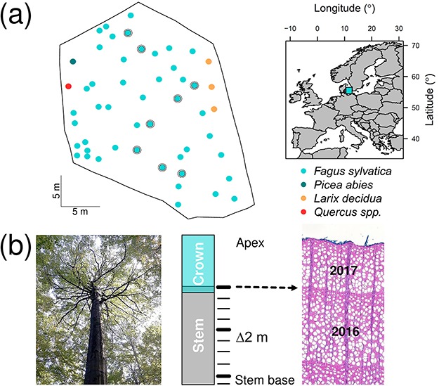
Sampling location and design. (a) A fixed forest plot (2460 m²) was established at the Sorø long-term ecological monitoring site (Central Zealand, Denmark). Each dot represents a plot tree (≥10 cm diameter at breast height) and shaded circles mark ‘axial trees,’ on which regular interval sampling was performed. (b) Graphical representation of the regular interval sampling. Wood increment cores were sampled every 2 m along the stem axis, for which ring width (thin lines) and wood anatomical properties (thick lines) were measured (image of diffuse-porous anatomical structure of F. sylvatica).

Sample collection and ring-width measurements

We collected two increment cores of all living trees with a DBH ≥10 cm within the fenced area (hereafter called ‘plot trees’; Figure 1a). Cores were taken perpendicular to each other to account for circumferential growth variation and labeled using a Dave2000 device. For each plot tree, we recorded the species, social status, position, height of the tree (H_tree) and its crown base (using a Vertex IV, Haglöf, Sweden) and DBH (see Table S1 available as Supplementary Data at Tree Physiology Online). Additional measurements of DBH and H_tree were taken from trees outside the plot to cover the full DBH range needed to establish robust allometric relationships (Figure S1 available as Supplementary Data at Tree Physiology Online). Sample preparation followed standard dendrochronological techniques (Schweingruber 1996) to prepare, measure (Lintab 6 station and TSAP-Win software, Rinntech Inc.) and visually and statistically cross-date all tree-ring width series (using COFECHA; Holmes 1983). In case a core did not reach the pith, we performed a pith offset estimation based on the curvature of the last rings (Pirie et al. 2015).

Regular interval sampling was performed by a professional tree climber on a subset of eight dominant F. sylvatica trees to collect wood cores at 0.5 m, 1.3 m and then every 2 m until the height at which the main stem ends (Figure 1). We measured RW for each core from these ‘axial trees.’ Then, we selected three heights along the stem (breast height, mid-stem and top-stem) for high-precision wood anatomical and density measurements covering the 1996–2017 period (corresponding to the intense ecological monitoring at this site; Pilegaard et al. 2011).

Wood anatomical and density measurements

Quantitative wood anatomical analysis was used to determine cell-specific properties, including high-resolution measurements of inter- and intra-annual wood density (ρ; Prendin et al. 2017). Additionally, this approach allowed us to ascertain which wood anatomical property contributes most to the inter-annual variability in density (e.g., vessel and fiber lumen and cell wall area). For the three wood cores per axial tree, 10 to 12 μm-thick microsections were cut using a rotatory microtome (Leica RM2245, Leica Biosystems, Nussloch, Germany). The thin sections were stained with safranin and astra blue and permanently fixed on glass slides using Canada balsam (Gärtner et al. 2015). From each slide, digital images of radial anatomical properties (fibers and vessels) were taken for each ring within the 1996–2017 period using a slide scanner (Axio Scan Z1, Zeiss, Germany). The ROXAS software (von Arx and Carrer 2014) combined with Image-Pro Plus (Media Cybernetics, Rockville, MD, USA) allowed us to detect fibers and vessels automatically and manually from the images (von Arx et al. 2016). Cell lumen area (A in μm²), mean cell wall thickness (WT in μm) and cell radius of the long (α) and short (β) axis were measured for each detected fiber (A <150 μm²) and vessel (A ≥150 μm²), together with positional information relative to the ring boundary (see Peters et al. 2018). A density profile was established by dividing each tree ring in the processed image into 100-μm-wide sectors (s) parallel to the ring boundary and calculating the mean density per sector (ρ_s, assuming a fixed density of wall material expressed with γ = 1.504 g cm^-3; Kellogg et al. 1969) based on Eq. (1):

(1)

where the wall area of each cell (c) is calculated using WT and A (assuming an elliptical shape using α and β). We excluded the area of occasional larger rays wider than 50 μm (ray area in μm²; δ_s) within each sector, as our sampling design using 5-mm-wide cores does not allow quantification of the abundance of larger rays within each year in a representative way. In rare cases when automatic measurement of WT failed due to undetected neighboring fiber cells, the mean WT within a sector was used instead. Empty areas (excluding δ_s) due to unmeasured fiber cells in each sector were filled with fiber cells of average dimensions for that sector. To account for wedging and waving ring boundaries, sector width was reduced (increased) in narrower (wider) parts of the ring, while still averaging to an overall mean sector width of 100 μm. Additional bulk and annual wood density measurements using the water displacement and X-ray densitometry methods, respectively (Eschbach et al. 1995, Williamson and Wiemann 2010), were performed to benchmark our wood anatomical density (see Figure S2 available as Supplementary Data at Tree Physiology Online and associated text).

Axial changes in radial growth and wood density

To analyze the variability of RW and ρ along the stem axis (relates to hypotheses H1 and H2), the distance to the apex was calculated from each axial sampling interval between 1996 and 2017 (H_apex [m]; considering height growth over time by using the allometric relationship between height and DBH determined in situ and presented in Figure S1 available as Supplementary Data at Tree Physiology Online). We used H_apex instead of the absolute height where samples were taken because it has the advantage that the data are intercomparable between trees of different cambial age and H_tree, which was a prerequisite for our two-step analysis. In the first step, we assessed the relationship between RW and H_apex separately for each tree and year using linear regression models. The resulting intercepts and slopes provided a metric of how strong the axial changes in RW were in a given year. In a second step, we compared the strength of these axial changes to radial growth at breast height across all trees and years. For this, we constructed a linear mixed-effects model, in which the annual slopes were fitted against annual RW at breast height from the corresponding trees, with ‘tree’ included in the model as a random effect. To constrain the uncertainties associated with the fitted linear regression parameters, we performed a bootstrapped resampling analysis (1000 iterations with replacement). This analysis was performed using the ‘lme4’ package in R (Bates et al. 2014) and accounted for linear model assumptions (e.g., normality and homogeneity; Zuur et al. 2010). The same two-step analysis was then applied twice more for ρ and A_vessel.

Effects of axial growth variations on stem biomass increment

Two implicit assumptions are usually made when ABI_stem is derived from a combination of forest inventory data and tree-ring measurements taken only at breast height (Babst et al. 2014a): (i) the yearly variability in RW at breast height represents that of radial growth and volume increment of the entire stem; and (ii) ρ is constant within and along the stem. To test our hypothesis H3 that these assumptions introduce biases in ABI_stem estimates, we assessed the impact of axial variability in RW and ρ on ABI_stem for both the axial trees and the entire plot. We thereby considered all four possible scenarios of accounting for or discarding this axial variability: (i) both are fixed to breast height (RW_fix × ρ_fix); (ii) RW is fixed to breast height and ρ varies along the stem (RW_fix × ρ_var); (iii) ρ is fixed to breast height and RW varies along the stem (RW_var × ρ_fix); and (iv) both vary along the stem (RW_var × ρ_var).

These scenarios were implemented in Eq. (2), given that ABI_stem of a specific year (y) is determined by the stem volume (V_stem) change in that year and by ρ of the newly formed wood.

(2)

Our regular interval sampling thereby provided us with RW measurements at different sampling heights (i), which we progressively subtracted from the respective outer stem radii measured in 2017 (see Figure S4 available as Supplementary Data at Tree Physiology Online) to reconstruct the stem radius for each year between 1996 and 2017. Then, we linearly interpolated between the radii along the stem axis for each year, assuming a conic stem shape between the sampling heights. The volume of these stem segments was calculated for each year () in two ways: (i) by subtracting for all segments the average RW measured at breast height to simulate the RW_fix scenario and (ii) using the RW measurements from that specific i (i.e., the RW_var scenario). ABI_stem was then calculated according to Eq. (2), using either the mean ρ determined by the water displacement method for the respective axial tree (the ρ_fix scenario; see Figure S4 available as Supplementary Data at Tree Physiology Online) or the inter-annual time series of ρ obtained from the wood anatomical density profiles at different sampling heights (ρ_var scenario).

To determine ABI_stem for the entire plot, we estimated the outer stem profile in 2017 of all plot trees, using a taper function dependent upon H_apex and DBH (see Figure S6 available as Supplementary Data at Tree Physiology Online). The total stem length in 2017 was equal to the measured crown base height in the field (see Table S1 available as Supplementary Data at Tree Physiology Online). The annual stem radius was reconstructed based on RW at breast height and using the proportional method proposed by Bakker (2005) to account for circumferential variation. As described above for the axial trees, we also applied the four scenarios of calculating ABI_stem for all plot trees (RW_fix × ρ_fix, RW_fix × ρ_var, RW_var × ρ_fix and RW_var × ρ_var). For the RW_var scenario, the RW measurements at breast height of all plot trees were corrected for the patterns found within the axial trees (see Figure 2) while accounting for changes in the distance to the apex due to height growth (see Figure S1 available as Supplementary Data at Tree Physiology Online). For ρ_fix a fixed value of 0.634 g cm^-3 was used (see Figure S4 available as Supplementary Data at Tree Physiology Online), while ρ_var accounted for inter-annual variability obtained from the wood anatomical measurements. The ABI_stem of all axial and plot trees was then summed up to the plot level and expressed on a per-area basis (kg ha^-1). Finally and for comparison, the ABI_stem for each tree and the entire plot was also determined using three different generalized allometric biomass equations for F. sylvatica (Forrester et al. 2017, see Note S1 available as Supplementary Data at Tree Physiology Online).

Figure 2.

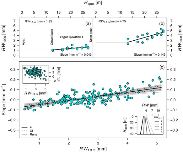
Variability in ring width (RW) as a function of distance to the apex (H_apex). As an example, the linear relationship between RW and H_apex is presented for F. sylvatica tree number 4 for an unfavorable (a) (low RW_{1.3 m} in the drought year 1996) and a favorable growth year (b) (high RW_{1.3 m} in 1998). The slopes and intercepts (int.) obtained from all axial trees and years are plotted against RW_{1.3 m} in (c). The lower right inset indicates the resulting RW patterns for a specific RW_{1.3 m}, according to the fitted linear regression of the slope with a fixed intercept. Significant linear relationships at P < 0.05 are indicated with solid lines. Uncertainty is presented by fitting linear models using bootstrap resampling (n = 1000; gray lines). The mean (solid black line) and the 95% confidence interval are provided from all simulations (dashed black lines at 2.5 and 97.5%).

Climatic drivers of radial growth and wood density variability

To identify the relevant climatic variables that drive temporal variability in RW and ρ, climate correlation analyses were performed for both plot trees and axial trees. For this purpose, we constructed site chronologies from all measurements at breast height (see Table S2 available as Supplementary Data at Tree Physiology Online for RW and Table S3 for ρ, available as Supplementary Data at Tree Physiology Online) using a cubic smoothing spline detrending with a 50% frequency cutoff response at 30 years (using dplR; see Bunn 2008). This procedure removed the biological age/size trend and other low-frequency variability (Cook et al. 1990, Peters et al. 2015). We also revisited earlier X-ray densitometry measurements from the same site (Babst et al. 2014b) to be able to assess the climate response of ρ over a longer time period starting in 1930.

We calculated Pearson’s correlation coefficients between the resulting RW and ρ chronologies and monthly mean temperature (in °C) and precipitation sum (in mm) derived from the CRU 3.23 gridded dataset (Harris et al. 2014). This climate response was assessed for two separate periods starting (i) in 1930 (maximum length of RW and X-ray ρ series with ≥10 individuals) to identify the overall temperature and water limitations on tree growth at our site and (ii) in 1996 (covering RW and ρ derived from wood anatomical data) to assess hypothesis H2 in more detail. Additionally, we performed an uncertainty analysis on the climate–growth correlations to confirm that the shorter records from the axial trees (starting in 1996) matched with the variability of the longer time series (starting in 1930) and showed a similar climatic response (see Figure S3 available as Supplementary Data at Tree Physiology Online). Because Babst et al. (2014a) showed that RW responds to summer drought at this site, relatively wet and dry summers (June, July and August) were individually assessed. Wet and dry summers were defined above the 90th (204.6 mm) and below the 10th (139.7 mm) percentile of total summer precipitation over the period from 1930–2014, respectively.

Results

Ring-width variability along the stem

No significant relationship was found between mean RW and H_apex for the axial trees (slope = 0.014 mm m^-1, P = 0.391; including a random slope and intercept for the tree; Figure S6a available as Supplementary Data at Tree Physiology Online). However, the coefficient of variation (CV) for the period 1996–2017 decreased significantly towards the apex (slope = 0.005 m^-1, P = 0.007; Figure S7b available as Supplementary Data at Tree Physiology Online), indicating that the year-to-year variability in RW is dampened towards higher stem parts. When isolating individual years and assessing the relationship between RW and H_apex, we did find significant slopes (P < 0.05) that were more shallow when RW at breast height (RW_{1.3 m}) was smaller (e.g., when comparing Figure 2a with Figure 2b, see Figure S8 available as Supplementary Data at Tree Physiology Online for isolated year-specific relationships between RW and H_apex). These slopes obtained from all axial trees and years had a strong significant relationship with RW_{1.3 m} (slope = 0.03 mm m^-1 mm^-1; P = 0.005; including a random slope and intercept for the tree), where a disproportionately larger RW is expected closer to the stem base during favorable growth years (Figure 2c, the intercept of the relationship was not significant: slope = −0.0863 mm m^-1, P = 0.71). Conversely and to our surprise, negative slopes between RW and H_apex were found during years when RW at breast height was below 2 mm (Figure 2c), indicating larger RW at the top than at the bottom of the stem.

Variability of wood anatomical density

A total of 24 wood cores from the eight axial trees were analyzed from 1996 to 2017 for wood anatomical properties, including all vessels and detected fibers (see Table S1 available as Supplementary Data at Tree Physiology Online). No significant relationship was found between mean annual ρ and H_apex (P = 0.469, including a random slope and intercept for the tree; Figure 3a). However, as expected from a hydraulic perspective, a significant tapering of the vessel lumen area (A_vessel) was found when moving closer to the apex (slope = 22.720 μm^-2 m^-1, P < 0.001; Figure 3b). When isolating individual years, the slope between ρ and H_apex was generally not significantly different from 0 g cm^-3 m^-1 (P > 0.05; Figure 3c). Thus, although vessels become smaller towards the apex, ρ does not change significantly. An explanation for this is that the number of vessels per unit area increases with smaller RW and compensates for smaller vessels towards the apex (log₁₀(ρ_vessel [# mm⁻²]) = 3 ^× log₁₀(RW [mm])−1.176, P < 0.001; see Figure S9 available as Supplementary Data at Tree Physiology Online). Regarding fiber ρ, there was an increasing trend towards the apex, but this relationship between H_apex and mean annual fiber ρ was just below the significance threshold (P = 0.0519). Moreover, the axial change in maximum cell wall thickness of the fibers was not significant (P = 0.095; linear mixed-effect modeling with the tree as a random effect). Additionally, the mean inter-annual variability in total ring ρ did not show a strong relationship with the variability in fiber ρ (Pearson’s r = 0.165, P = 0.4645; see Figure S2b available as Supplementary Data at Tree Physiology Online).

Figure 3.

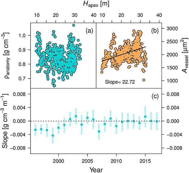
Relationship between anatomically derived wood density (ρ_anatomy), vessel lumen area (A_vessel) and the distance to the apex (H_apex). (a) Annual mean ρ_anatomy and (b) A_vessel measurements for all axial trees (from 1996–2017) are plotted against H_apex. The significant linear relationship in (b) (P < 0.001) is indicated with a solid black line. (c) Slope of a linear mixed-effect model when analyzing ρ_anatomy against H_apex for each individual year. The standard error of the slope is provided with bold lines, and significant relationships are indicated with a black circle.

Correlation analyses between climate, ring width and density

At the plot level, the detrended RW series sampled at breast height from all 46 F. sylvatica trees showed a mean inter-series correlation of 0.435 over the common period 1930–2017 (see Table S2 available as Supplementary Data at Tree Physiology Online). The resulting RW chronology showed a strong positive relationship with June precipitation (common period 1930–2014; r = 0.48, P < 0.001) and a negative relationship with July temperatures (r = −0.30, P = 0.006; Table 1). By contrast, the X-ray ρ chronology revealed higher ρ values with warmer temperatures (r = 0.33, P = 0.003) and lower precipitation in May (common period 1930–2009; r = −0.39; P < 0.001; Table 1). When considering only RW and wood anatomical ρ measurements for the axial trees, less pronounced correlations were found (likely due to lower sample size and the shorter observation period; see Figure S3 available as Supplementary Data at Tree Physiology Online) that were still significantly positive between RW and June precipitation and between ρ and May temperature (common period 1996–2014; Table 1). For these trees, a strong positive relationship was also found between the variability in RW and ρ, with wider rings being denser (slope = 0.115, r = 0.80 and P < 0.001). When comparing the raw RW and ρ only at breast height of the axial trees, again a significant positive relationship emerged (slope = 0.013 g cm^-3 mm^-1, P = 0.008; including a random intercept and slope of the tree).

Table 1.

Relationships between ring width (RW) and wood density (ρ) with monthly mean air temperature (Temp) and monthly summed precipitation (Prec). The number of trees included (n), Pearson’s correlation coefficient (r), slope of the linear regression and significance (P) are presented. A total of four chronologies were assessed, constructed from (i) all ring-width measurements at breast height (1.3 m) from the plot trees (RW_plot), (ii) X-ray ρ measurements from Babst et al. (2014b) for the same site (ρ_plot), (iii) the RW at breast height from the axial trees (RW_axial) and (iv) the wood anatomical ρ measurement at breast height from the axial trees (ρ_axial)

Chronology	n	Years	Variable	r	Slope	P-value
RWplot	46	1930–2014	TempJune	−0.23	−0.029	0.036
			TempJuly	−0.30	−0.029	0.006
			PrecJune	0.48	0.003	0.000
ρplot	29	1930–2009	TempMay	0.33	0.006	0.003
			TempJune	0.27	0.005	0.014
			PrecMay	−0.39	0.000	0.000
RWaxial	8	1996–2014	TempJune	0.06	0.015	0.794
			TempJuly	−0.34	−0.044	0.157
			PrecJune	0.75	0.007	0.000
ρaxial	8	1996–2014	TempMay	0.54	0.016	0.017
			TempJune	0.09	0.003	0.721
			PrecMay	−0.39	−0.001	0.102

Impact of variability in ring width and density on aboveground biomass increment of the stem

We tested four scenarios of considering (‘var’) or discarding (‘fix’) axial variability in RW and ρ when estimating ABI_stem. In scenario 1 that kept both parameters fixed at breast height (RW_fix × ρ_fix), the axial trees showed an average ABI_stem of 28.3 ± 10.4 kg tree^-1 year^-1 between 1996 and 2017. In scenario 2 that allowed for axial variability in RW but not in ρ (RW_var × ρ_fix), the estimated ABI_stem was on average smaller by −1.16 ± 1.98 kg tree^-1 year^-1 (Figure 4a). When looking at relatively wetter summers (2002, 2007 and 2011), this difference to scenario 1 increased to a significant −3.13 kg tree^-1 (P = 0.03; Student’s t-test), whereas dry summers (1996 and 2013) showed only a small difference of −0.34 kg tree^-1 (P = 0.78). In scenario 3, which allowed for axial variability in ρ but not in RW (RW_fix × ρ_var), the average difference in ABI_stem compared with scenario 1 was 0.10 ± 0.88 kg tree^-1 year^-1 and thus very small. In scenario 4, where axial variability in both parameters was considered (RW_var × ρ_var), ABI_stem was on average − 1.09 ± 1.47 kg tree^-1 year^-1 smaller than in scenario 1. Taken together, we found that discarding axial variability in RW leads to a significant overestimation of ABI_stem in wet summers, whereas the impact of axial variability in ρ was negligible.

Figure 4.

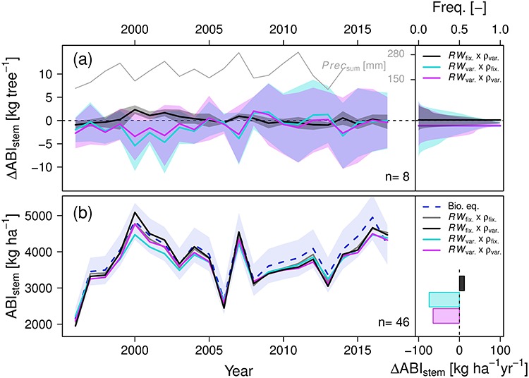
Aboveground biomass increment of entire stems (ABI_stem) when either considering axial variability in ring width (RW) and wood density (ρ) or keeping them fixed at breast height. Either RW variability at breast height was used to reconstruct the stem radius (RW_fix), or RW was allowed to vary according to the distance from the apex (RW_var). For ρ, either a fixed value of 0.634 g cm^-3 was applied (ρ_fix), or the ρ time series derived from wood anatomical measurement at breast height (ρ_var) were used. (a) The average ∆ABI_stem from all axial trees is shown related to the RW_fix × ρ_fix scenario. Cumulative summer precipitation is additionally displayed. The mean of all trees is indicated with a bold line, and the shaded area shows the standard deviation. In the right panel, the color legend is provided, along with a histogram of ∆ABI_stem across all years with a bold line indicating the mean. (b) ABI_stem of the entire plot for the average of three allometric biomass equations (shaded area indicates the standard deviation) and when including or excluding axial variability in RW and ρ. The panel on the right presents the color legend and ∆ABI_stem for the plot.

At the plot level, the three allometric biomass equations (see Note S1 available as Supplementary Data at Tree Physiology Online) showed an average ABI_stem of 3870 ± 661 kg ha^-1 year^-1, albeit with a considerable spread (average difference in standard deviation of 955 kg ha^-1 year^-1 or 25%; Figure 4b). The inter-annual variability in ABI_stem derived from the allometric biomass equations matched well with that obtained from the different scenarios described above (Figure 4b). When comparing ABI_stem of the plot resulting from scenario 1 (RW_fix × ρ_fix) with that from scenario 2 (RW_var × ρ_fix), the inter-annual variability appeared dampened in the latter, with an average difference in ABI_stem of −74 ± 116 kg ha^-1 year^-1 (−2%; P = 0.007). Similar to the tree level (see above), this difference was smaller when additionally considering the inter-annual variability in ρ (−64 ± 88 kg ha^-1 year^-1 or − 1.7% in scenario 4 compared with scenario 1; P = 0.003). Additionally, when comparing the standard deviation of the time series for ABI_stem in scenario 1 (RW_fix × ρ_fix) and scenario 4 (RW_var × ρ_var), it was 41 g ha¹ year¹ smaller in the latter.

Discussion

Radial growth variability along the stem

This study combined functional and quantitative perspectives on wood formation along the stem of mature F. sylvatica trees to elucidate how radial growth, wood density, climate and climatic extremes interact to shape the aboveground biomass increment. Our results specifically indicate that climate mediates the axial changes in radial growth. Wetter (drier) summers trigger disproportionately larger (smaller) RW at breast height (RW_plot in Table 1), which subsequently induces a stronger (weaker) gradient in RW towards higher stem parts (Figure 2). It is well known that unfavorable growing conditions like summer droughts (low June precipitation and high temperatures at our study site; Table 1) reduce RW in F. sylvatica (e.g., Bouriaud et al. 2004, Bosela et al. 2016, Bhuyan et al. 2017). Our results now provide evidence that this reduction in RW is less pronounced at the top of the stem compared with the stem base, confirming our second hypothesis H2. In extreme cases (RW at breast height <2 mm), we even found that radial growth closer to the apex exceeded that in lower stem sections. As a consequence, growth variability and climate sensitivity appear to be dampened closer to the apex for F. sylvatica (see also Bouriaud et al. 2005a). Some previous studies on axial growth variability in coniferous species have observed a stronger RW reduction at breast height vs closer to the apex only during (late) summer droughts, whereas during dry and warm early-season conditions, RW closer to the apex was equally reduced (Chhin et al. 2010, van der Maaten and Bouriaud 2012). These seasonally divergent responses possibly point to a change in priority from radial growth in higher stem parts during the early growing season towards radial growth (and higher climatic sensitivity) in lower parts later in the season.

Differences in the axial distribution of assimilates (Lacointe 2000) can provide a physiological explanation for the environmental regulation of RW along the stem (as discussed by Farrar 1961). Flow of assimilates is driven by the interplay between turgor gradients regulated by water availability and osmotic gradients generated by differences in sugar concentration between the regions of phloem loading (i.e., leaves) and unloading (i.e., roots; Münch’s 1930, De Schepper and Steppe 2010). This osmotic gradient is distorted during droughts due to reduced production of assimilates and lower water availability, which is hypothesized to lower phloem conductivity (Ryan et al. 2014) and slows down the transport of assimilates to the lower parts of the stem (e.g., Sevanto et al. 2003). This reduction in available assimilates impacts growth directly due to the lack of carbon or turgidity required in the cambium for cell production and enlargement (Lockhart 1965, Cosgrove 1993, De Schepper and Steppe 2010, Lazzarin et al. 2018). An alternative explanation for the difference in radial growth along the stem is the apical control over the initiation and cessation of wood formation (e.g., due to auxin gradients; Larson 1963, Rathgeber et al. 2011). Accordingly, growth closer to the apex starts earlier and is thus less susceptible to summer drought, as large parts of the ring have already been formed by that time. Yet, this explanation is challenged by studies on a variety of different species that did not find a difference in radial growth initiation with stem height (Sunberg et al. 1991, Lachaud et al. 1999, Bouriaud et al. 2005b, Anfodillo et al. 2012). Further physiological studies in combination with mechanistic modeling (Steppe et al. 2015) are likely needed to elucidate the driving mechanism behind RW patterns along the stem. Nevertheless, our results suggest that F. sylvatica prioritizes growth in the upper part of the stem during unfavorable conditions (Figure 2), supporting a resource allocation rule with lesser priority for the stem base (e.g., Lacointe 2000, Schippers et al. 2015).

Anatomical basis of wood density variability along the stem

Our findings suggest that in F. sylvatica, inter-annual variability in ρ is driven by a combination of vessel area (A_vessel) and the number of vessels per unit area within the ring. Although the wood anatomical basis behind inter-annual variability in wood density parameters (e.g., maximum latewood density; Esper et al. 2012) has been extensively studied for conifers (Wang et al. 2002, Pritzkow et al. 2014, Björklund et al. 2017), this study is among the first to elucidate the wood anatomical basis behind the inter-annual variability in ρ for a diffuse-porous species. In contrast to coniferous species where ρ tends to decrease with increasing RW (Bouriaud et al. 2005b, Franceschini et al. 2013), we find that F. sylvatica significantly increases ρ with larger RW by about 0.013 g cm^-3 per mm. This increase can be attributed to the number of vessels per unit wood area within the ring, which decreases with increasing RW, whereas the proportion of fibers increases (see Figure S9 available as Supplementary Data at Tree Physiology Online). These results contrast with findings from Bouriaud et al. (2004), who found no relationship, and with Pretzsch et al. (2018), who found slight reductions in ρ with increasing RW in F. sylvatica. The lack of a clear relationship between ρ and RW in this literature could be due to the use of X-ray densitometry (as opposed to wood anatomical measurements in our study), where technical issues with cell alignment, lower image accuracy and measurement bands overlapping with two rings could have distorted the signal (Parker and Meleskie 1970, Park and Telewski 1993, Jacquin et al. 2017).

Apart from its co-dependence on RW, variability in ρ can also be caused by different climatic drivers (e.g., Briffa et al. 2002, Frank and Esper 2005, Cuny et al. 2015). At our site, higher ρ was associated with drier and warmer climatic conditions in May (Table 1), which likely coincide with an earlier start of the growing season. A warm spring may also enhance photosynthetic rates and provide the tree with additional time and resources to develop more latewood (as described for conifers in Lupi et al. 2010, e.g., for F. sylvatica wood with relatively more fibers and less vessels). Skomarkova et al. (2006) confirm this hypothesis, showing that maximum ρ of F. sylvatica from central Germany showed a positive trend with May and July temperatures. The latter relationship was absent at our site, likely due its susceptibility to summer drought (Table 1). Surprisingly, no significant relationship was found between H_apex and ρ (Figure 3a and c). We must therefore reject hypothesis H1, despite a significant increase in vessel lumen area (A_vessel) with increasing H_apex (Figure 3b). The A_vessel tapering from the stem base towards the apex is in agreement with West et al. (1999), showing a universal vessel diameter scaling with stem length driven by hydraulics. It thus appears that vessel tapering in F. sylvatica counteracts the expected reduction in ρ with decreasing RW (positive relationship) towards the upper part of the stem. These results compared with earlier findings from conifer species hint at fundamentally different responses of ρ during favorable and unfavorable growing conditions, depending on the complexity of the wood structure (e.g., vessels and fibers in ring-/diffuse-porous species vs only tracheids in conifers; e.g., Guilley et al. 1999, Bergès et al. 2000, Franceschini et al. 2013). From a functional perspective, the fact that the proportion of fibers decreases along the axial direction and during unfavorable growing conditions (e.g., smaller RW) hints at a priority of F. sylvatica to maintain hydraulic conductivity at the expense of mechanical support (Chave et al. 2009). Yet more detailed wood anatomical analyses will be required to further elucidate climatic impacts on wood structure and function (e.g., Prendin et al. 2018).

Regulation of stem biomass and uncertainties

Our four scenarios of including or excluding axial variability in RW and ρ when calculating ABI_stem indicated a positive bias in individual trees mainly during years with favorable growing conditions (e.g., 2002, 2007 and 2011; Figure 4). When scaled to the plot level and integrated across all years, this translates into a minor overestimation of 65 kg ha^-1 year^-1 (~2%) for the period 1996–2017 (Figure 4b), although the standard deviation around this estimate is considerable. This positive bias can be significantly higher in individual years with a wet summer (e.g., 204 kg ha^-1 in the year 2002), but still falls within the uncertainty in ABI_stem imposed by the three allometric biomass equations (Figure 4b). We acknowledge that these allometric biomass equations may not be ideal benchmarks for our ABI_stem estimates, because they are known as an important contributor to the overall uncertainty in forest productivity estimates (e.g., Alexander et al. 2018). Additionally, uncertainty in height measurements (e.g., Larjavaara and Muller-Landau 2013) could impact our height (DBH) allometric function and H_apex (see Figure S1 available as Supplementary Data at Tree Physiology Online). Finally, as increment cores do not always reach the center of the stem, pith offset estimations have to be performed (Pirie et al. 2015), which potentially impact the diameter reconstruction. Nevertheless, we must reject hypothesis H3 based on our data and conclude that axial variability in RW and ρ does not strongly bias plot-level ABI_stem estimates derived from breast height measurements in F. sylvatica. Hence, RW variability along the stem will likely not explain the discrepancies found between in situ measurements of aboveground biomass increment and net ecosystem productivity (Babst et al. 2014b), nor its different climatic sensitivity compared with dynamic global vegetation model output (Klesse et al. 2018).

Conclusion

Our combined functional and quantitative assessment of wood production has shown that variation in volume and not wood density is the main source of axial variability in the stem biomass increment of F. sylvatica. The reduced growth variability and climate sensitivity in higher compared with lower stem sections may thereby indicate preferential carbon allocation to proximal sinks under unfavorable (i.e., summer drought) conditions. In turn, growth at the stem base increased disproportionately in favorable years, leading to an overestimation of ABI_stem when considering only measurements taken at breast height. However, this significant positive bias at the tree level turned out to be negligible when scaling to the plot level and averaging over the study period (~2% overestimation of ABI_stem). On one hand, this result validates aboveground biomass reconstructions for F. sylvatica from classic field sampling (e.g., Babst et al. 2014b). On the other hand, more research is clearly needed to unravel the dynamics of carbon allocation to various structural and nonstructural sinks, as well as their turnover rates. We recommend that this be done using a similar combination of wood anatomical and biometric measurements, ideally supported by mechanistic modeling (Zuidema et al. 2018, Fatichi et al. 2019). This framework will help to further elucidate the wood anatomical properties driving RW and ρ in different tree species, reduce scaling uncertainties associated with tree-ring data (Babst et al. 2018) and refine our understanding of forest carbon fixation.

Conflict of interest

The authors declare that they have no conflict of interest.

Funding

This work was part of the project ‘Inside out’ (#POIR.04.04.00–00-5F85/18–00) funded by the HOMING program of the Foundation for Polish Science co-financed by the European Union under the European Regional Development Fund. The work was also supported by the EU-H2020 program (grant 640176, ‘BACI’) and by the Swiss National Science Foundation Early Postdoc. Mobility (grant P2BSP3_184475).

References

- Alexander MR, Rollinson CR, Babst F, Trouet V, Moore DJP (2018) Relative influences of multiple sources of uncertainty on cumulative and incremental tree-ring-derived aboveground biomass estimates. Trees Struct Funct 32:265–276. [Google Scholar]
- Anfodillo T, Carraro V, Carrer M, Fior C, Rossi S (2006) Convergent tapering of xylem conduits in different woody species. New Phytol 169:279–290. [DOI] [PubMed] [Google Scholar]
- Anfodillo T, Deslauriers A, Menardi R, Tedoldi L, Petit G, Rossi S (2012) Widening of xylem conduits in a conifer tree depends on the longer time of cell expansion downwards along the stem. J Exp Bot 63:837–845. [DOI] [PMC free article] [PubMed] [Google Scholar]
- Babst F, Bouriaud O, Alexander R, Trouet V, Frank D (2014a) Toward consistent measurements of carbon accumulation: a multi-site assessment of biomass and basal area increment across Europe. Dendrochronologia 32:153–161. [Google Scholar]
- Babst F, Bouriaud O, Papale D et al. (2014b) Above-ground woody carbon sequestration measured from tree rings is coherent with net ecosystem productivity at five eddy-covariance sites. New Phytol 201:1289–1303. [DOI] [PubMed] [Google Scholar]
- Babst F, Bodesheim P, Charney N et al. (2018) When tree rings go global: challenges and opportunities for retro- and prospective insight. Quat Sci Rev 197:1–20. [Google Scholar]
- Bakker JD. (2005) A new, proportional method for reconstructing historical tree diameters. Can J For Res 35:2515–2520. [Google Scholar]
- Bar-On YM, Phillips R, Milo R (2018) The biomass distribution on earth. Proc Natl Acad Sci USA 115:6506–6511. [DOI] [PMC free article] [PubMed] [Google Scholar]
- Bates D, Mächler M, Bolker B, Walker S (2014) Fitting linear mixed-effects models using lme4. J Stat Softw 67:1–48. [Google Scholar]
- Bergès L, Dupouey JL, Franc A (2000) Long-term changes in wood density and radial growth of Quercus petraea Liebl. In northern France since the middle of the nineteenth century. Trees Struct Funct 14:398–408. [Google Scholar]
- Bhuyan U, Zang C, Menzel A (2017) Different responses of multispecies tree ring growth to various drought indices across Europe. Dendrochronologia 44:1–8. [Google Scholar]
- Björklund J, Seftigen K, Schweingruber F et al. (2017) Cell size and wall dimensions drive distinct variability of earlywood and latewood density in northern hemisphere conifers. New Phytol 216:728–740. [DOI] [PubMed] [Google Scholar]
- Bosela M, Štefančík I, Petráš R, Vacek S (2016) The effects of climate warming on the growth of European beech forests depend critically on thinning strategy and site productivity. Agric For Meteorol 222:21–31. [Google Scholar]
- Bouriaud O, Bréda N, Moguédec G, Nepveu G (2004) Modelling variability of wood density in beech as affected by ring age, radial growth and climate. Trees Struct Funct 18:264–276. [Google Scholar]
- Bouriaud O, Bréda N, Dupouey J-L, Granier A (2005a) Is ring width a reliable proxy for stem-biomass increment? A case study in European beech. Can J For Res 35:2920–2933. [Google Scholar]
- Bouriaud O, Leban JM, Bert D, Deleuze C (2005b) Intra-annual variations in climate influence growth and wood density of Norway spruce. Tree Physiol 25:651–660. [DOI] [PubMed] [Google Scholar]
- Bouriaud O, Teodosiu M, Kirdyanov AV, Wirth C (2015) Influence of wood density in tree-ring-based annual productivity assessments and its errors in Norway spruce. Biogeosciences 12:6205–6217. [Google Scholar]
- Briffa KR, Osborn TJ, Schweingruber FH, Jones PD, Shiyatov SG, Vaganov EA (2002) Tree-ring width and density data around the northern hemisphere: part 1, local and regional climate signals. Holocene 12:737–757. [Google Scholar]
- Bunn AG. (2008) A dendrochronology program library in R (dplR). Dendrochronologia 26:115–124. [Google Scholar]
- Castagneri D, Petit G, Carrer M (2015) Divergent climate response on hydraulic-related xylem anatomical traits of Picea abies along a 900-m altitudinal gradient. Tree Physiol 35:1378–1387. [DOI] [PubMed] [Google Scholar]
- Chave J, Coomes D, Jansen S, Lewis SL, Swenson NG, Zanne AE (2009) Towards a worldwide wood economics spectrum. Ecol Lett 12:351–366. [DOI] [PubMed] [Google Scholar]
- Chen G, Yang Y, Robinson D (2013) Allocation of gross primary production in forest ecosystems: Allometric constraints and environmental responses. New Phytol 200:1176–1186. [DOI] [PubMed] [Google Scholar]
- Chhin S, Hogg EH, Lieffers VJ, Huang S (2010) Growth-climate relationships vary with height along the stem in lodgepole pine. Tree Physiol 30:335–345. [DOI] [PubMed] [Google Scholar]
- Cook ER, Briffa KR, Shiyatov S, Mazepa V (1990) Tree-ring standardization and growth-trend estimation In: Cook ER, Kairiukstis LA (eds) Methods of dendrochronology: applications in the environmental sciences. Kluwer Academic Publishers, Dordrecht, The Netherlands, pp 104–123. [Google Scholar]
- Cosgrove DJ. (1993) Water uptake by growing cells: an assessment of the controlling roles of wall relaxation, solute uptake, and hydraulic conductance. Int J Plant Sci 154:10–21. [DOI] [PubMed] [Google Scholar]
- Cuny HE, Rathgeber CBK, Frank D et al. (2015) Woody biomass production lags stem-girth increase by over one month in coniferous forests. Nat Plants 1:1–6. [DOI] [PubMed] [Google Scholar]
- Cuny HE, Fonti P, Rathgeber CBK, Arx G, Peters RL, Frank D (2019) Couplings in cell differentiation kinetics mitigate air temperature influence on conifer wood anatomy. Plant Cell Environ 42:1222–1232. [DOI] [PubMed] [Google Scholar]
- Dalsgaard L, Mikkelsen TN, Bastrup-Birk A (2011) Sap flow for beech (Fagus sylvatica L.) in a natural and a managed forest - effect of spatial heterogeneity. J Plant Ecol 4:23–35. [Google Scholar]
- De Schepper V, Steppe K (2010) Development and verification of a water and sugar transport model using measured stem diameter variations. J Exp Bot 61:2083–2099. [DOI] [PubMed] [Google Scholar]
- Dietze MC, Sala A, Carbone MS, Czimczik CI, Mantooth JA, Richardson AD, Vargas R (2014) Nonstructural carbon in Woody plants. Annu Rev Plant Biol 65:667–687. [DOI] [PubMed] [Google Scholar]
- Dye A, Plotkin AB, Bishop D, Pederson N, Poulter B, Hessl A (2016) Comparing tree-ring and permanent plot estimates of aboveground net primary production in three eastern U.S. forests. Ecosphere 7:1–13. [Google Scholar]
- Eschbach W, Nogler P, Schär E, Schweingruber FH (1995) Technical advances in the radiodensitometrical determination of wood density. Dendrochronologia 13:155–168. [Google Scholar]
- Esper J, Frank DC, Timonen M et al. (2012) Orbital forcing of tree-ring data. Nat Clim Chang 2:862–866. [Google Scholar]
- Farrar JL. (1961) Longitudinal variation in the thickness of the annual ring. For Chron 37:323–349. [Google Scholar]
- Fatichi S, Pappas C, Zscheischler J, Leuzinger S (2019) Modelling carbon sources and sinks in terrestrial vegetation. New Phytol 221:652–668. [DOI] [PubMed] [Google Scholar]
- Forrester DI, Tachauer IHH, Annighoefer P et al. (2017) Generalized biomass and leaf area allometric equations for European tree species incorporating stand structure, tree age and climate. For Ecol Manage 396:160–175. [Google Scholar]
- Franceschini T, Longuetaud F, Bontemps JD, Bouriaud O, Caritey BD, Leban JM (2013) Effect of ring width, cambial age, and climatic variables on the within-ring wood density profile of Norway spruce Picea abies (L.) Karst. Trees Struct Funct 27:913–925. [Google Scholar]
- Frank D, Esper J (2005) Characterization and climate response patterns of a high-elevation, multi-species tree-ring network in the European alps. Dendrochronologia 22:107–121. [Google Scholar]
- Friend AD, Patrick AHE, Tim F, Rathgeber CBK, Richardson AD, Turton RH (2019) On the need to consider wood formation processes in global vegetation models and a suggested approach. Ann For Sci 76:49. [Google Scholar]
- Fritts HC, Smith DG, Budelsky CA, Cardis JW (1965) The variability of ring characteristics within trees as shown by a reanalysis of four ponderosa pine. Tree Ring Bull 27:3–18. [Google Scholar]
- Gärtner H, Lucchinetti S, Schweingruber FH (2015) A new sledge microtome to combine wood anatomy and tree-ring ecology. IAWA J 36:452–459. [Google Scholar]
- Gea-Izquierdo G, Guibal F, Joffre R, Ourcival JM, Simioni G, Guiot J (2015) Modelling the climatic drivers determining photosynthesis and carbon allocation in evergreen Mediterranean forests using multiproxy long time series. Biogeosciences 12:3695–3712. [Google Scholar]
- Guillemot J, Francois C, Hmimina G, Dufrêne E, Martin-StPaul NK, Soudani K, Marie G, Ourcival JM, Delpierre N (2017) Environmental control of carbon allocation matters for modelling forest growth. New Phytol 214:180–193. [DOI] [PubMed] [Google Scholar]
- Guilley É, Hervé JC, Huber F, Nepveu G (1999) Modelling variability of within-ring density components in Quercus petraea Liebl. With mixed-effect models and simulating the influence of contrasting silvicultures on wood density. Acta Med Bulg 56:449–458. [Google Scholar]
- Harris I, Jones PD, Osborn TJ, Lister DH (2014) Updated high-resolution grids of monthly climatic observations - the CRU TS3.10 dataset. Int J Climatol 34:623–642. [Google Scholar]
- Hartmann F, Rathgeber C, Fournier M, Moulia B (2017) Modelling wood formation and structure: power and limits of a morphogenetic gradient in controlling xylem cell proliferation and growth. Ann For Sci 74:1–15. [Google Scholar]
- He Y, Peng S, Liu Y et al. (2019) Global vegetation biomass production efficiency constrained by models and observations. Glob Chang Biol 00:1–11. [DOI] [PubMed] [Google Scholar]
- Holmes RL. (1983) Computer-assisted quality control in tree-ring dating and measurement. Tree Ring Bull 43:69–78. [Google Scholar]
- Jacquin P, Longuetaud F, Leban JM, Mothe F (2017) X-ray microdensitometry of wood: a review of existing principles and devices. Dendrochronologia 42:42–50. [Google Scholar]
- Kellogg RM, Wangaard FF (1969) Variation in the cell-wall density of wood. Wood Fiber Sci 1:180–204. [Google Scholar]
- Kerhoulas LP, Kane JM (2012) Sensitivity of ring growth and carbon allocation to climatic variation vary within ponderosa pine trees. Tree Physiol 32:14–23. [DOI] [PubMed] [Google Scholar]
- Klesse S, Etzold S, Frank D (2016) Integrating tree-ring and inventory-based measurements of aboveground biomass growth: research opportunities and carbon cycle consequences from a large snow breakage event in the Swiss alps. Eur J For Res 135:297–311. [Google Scholar]
- Klesse S, Babst F, Lienert S et al. (2018) A combined tree-ring and vegetation model assessment of European forest growth sensitivity to inter-annual climate variability. Global Biogeochem Cycles 32:1226–1240. [Google Scholar]
- Körner C. (2017) A matter of tree longevity. Science 355:130–131. [DOI] [PubMed] [Google Scholar]
- Lachaud S, Catesson AM, Bonnemain JL (1999) Structure and functions of the vascular cambium. C R Acad Sci Paris 322:633–650. [DOI] [PubMed] [Google Scholar]
- Lacointe A. (2000) Carbon allocation among tree organs: a review of basic processes and representation in functional-structural tree models. Ann For Sci 57:521–533. [Google Scholar]
- Lapenis AG, Lawrence GB, Heim A, Zheng C, Shortle W (2013) Climate warming shifts carbon allocation from stemwood to roots in calcium-depleted spruce forests. Global Biogeochem Cycles 27:101–107. [Google Scholar]
- Larjavaara M, Muller-Landau HC (2013) Measuring tree height: a quantitative comparison of two common field methods in a moist tropical forest. Methods Ecol Evol 4:793–801. [Google Scholar]
- Larson PR. (1963) The indirect effect of drought on tracheid diameter in red pine. For Sci 9:52–62. [Google Scholar]
- Lazzarin M, Zweifel R, Anten N, Sterck FJ (2018) Does phloem osmolality affect diurnal diameter changes of twigs but not of stems in Scots pine? Tree Physiol 32:275–283. [DOI] [PubMed] [Google Scholar]
- Le Quéré C, Andrew RM, Friedlingstein P et al. (2018) Global carbon budget 2017. Earth Syst Sci Data 10:405–448. [Google Scholar]
- Li G, Harrison SP, Prentice IC, Falster D (2014) Simulation of tree-ring widths with a model for primary production, carbon allocation, and growth. Biogeosciences 11:6711–6724. [Google Scholar]
- Litton CM, Raich JW, Ryan MG (2007) Carbon allocation in forest ecosystems. Glob Chang Biol 13:2089–2109. [Google Scholar]
- Lockhart JA. (1965) An analysis of irreversible plant cell elongation. J Theor Biol 8:264–275. [DOI] [PubMed] [Google Scholar]
- Lupi C, Morin H, Deslauriers A, Rossi S (2010) Xylem phenology and wood production: resolving the chicken-or-egg dilemma. Plant Cell Environ 33:1721–1730. [DOI] [PubMed] [Google Scholar]
- Luyssaert S, Inglima I, Jung M et al. (2007) CO2 balance of boreal, temperate, and tropical forests derived from a global database. Glob Chang Biol 13:2509–2537. [Google Scholar]
- Mausolf K, Härdtle W, Hertel D, Leuschner C, Fichtner A (2019) Impacts of multiple environmental change drivers no growth of European beech (Fagus sylvatica): Forest history matters. Ecosystems. doi: 10.1007/s10021-019-00419-0. [DOI] [Google Scholar]
- Mcmurtrie RE, Dewar RC (2013) New insights into carbon allocation by trees from the hypothesis that annual wood production is maximized. New Phytol 199:981–990. [DOI] [PubMed] [Google Scholar]
- Münch E. (1930) Die stoffbewegunen in der Planze. JenaGustav Fischer. [Google Scholar]
- Olson ME, Anfodillo T, Rosell JA, Petit G, Crivellaro A, Isnard S, León-Gómez C, Alvarado-Cárdenas LO, Castorena M (2014) Universal hydraulics of the flowering plants: vessel diameter scales with stem length across angiosperm lineages, habits and climates. Ecol Lett 17:988–997. [DOI] [PubMed] [Google Scholar]
- Pan Y, Birdsey RA, Fang J et al. (2011) A large and persistent carbon sink in the World’s forests. Science 333:988–994. [DOI] [PubMed] [Google Scholar]
- Park WK, Telewski FW (1993) Measuring maximum latewood density by image analysis at the cellular level. Wood Fiber Sci 25:326–332. [Google Scholar]
- Parker ML, Meleskie KR (1970) Preparation of X-ray negatives of tree-ring specimens for dendrochronological analysis. Tree Ring Bull 30:11–22. [Google Scholar]
- Peters RL, Groenendijk P, Vlam M, Zuidema PA (2015) Detecting long-term growth trends using tree rings: a critical evaluation of methods. Glob Chang Biol 21:2040–2054. [DOI] [PubMed] [Google Scholar]
- Peters RL, Balanzategui D, Hurley AG, Arx G, Prendin AL, Cuny HE, Björklund J, Frank DC, Fonti P (2018) RAPTOR: row and position tracheid organizer in R. Dendrochronologia 47:10–16. [Google Scholar]
- Pilegaard K, Ibrom A, Courtney MS, Hummelshøj P, Jensen NO (2011) Increasing net CO2 uptake by a Danish beech forest during the period from 1996 to 2009. Agric For Meteorol 151:934–946. [Google Scholar]
- Pirie MR, Fowler AM, Triggs CM (2015) Assessing the accuracy of three commonly used pith offset methods applied to Agathis australis (kauri) incremental cores. Dendrochronologia 36:60–68. [Google Scholar]
- Prendin AL, Mayr S, Beikircher B, Von Arx G, Petit G (2018) Xylem anatomical adjustments prioritize hydraulic efficiency over safety as Norway spruce trees grow taller. Tree Physiol 38:1088–1097. [DOI] [PubMed] [Google Scholar]
- Prendin AL, Petit G, Carrer M, Fonti P, Björklund J, Von Arx G (2017) New research perspectives from a novel approach to quantify tracheid wall thickness. Tree Physiol 37:1–8. [DOI] [PubMed] [Google Scholar]
- Pretzsch H, Biber P, Schütze G, Kemmerer J, Uhl E (2018) Wood density reduced while wood volume growth accelerated in central European forests since 1870. For Ecol Manage 429:589–616. [Google Scholar]
- Pritzkow C, Heinrich I, Grudd H, Helle G (2014) Relationship between wood anatomy, tree-ring widths and wood density of Pinus sylvestris L. and climate at high latitudes in northern Sweden. Dendrochronologia 32:295–302. [Google Scholar]
- Rathgeber CBK, Rossi S, Bontemps JD (2011) Cambial activity related to tree size in a mature silver-fir plantation. Ann Bot 108:429–438. [DOI] [PMC free article] [PubMed] [Google Scholar]
- Rathgeber CBK, Cuny HE, Fonti P (2016) Biological basis of tree-ring formation: a crash course. Front Plant Sci 7:1–7. [DOI] [PMC free article] [PubMed] [Google Scholar]
- Ryan MG, Asao S, Way D (2014) Phloem transport in trees. Tree Physiol 34:1–4. [DOI] [PubMed] [Google Scholar]
- Schippers P, Sterck F, Vlam M, Zuidema PA (2015) Tree growth variation in the tropical forest: understanding effects of temperature, rainfall and CO2. Glob Chang Biol 21:2749–2761. [DOI] [PubMed] [Google Scholar]
- Schweingruber FH. (1996) Tree rings and environment - Dendroecology. Paul Haupt, Bern, Switzerland. [Google Scholar]
- Sevanto S, Vesala T, Perämäki M, Nikinmaa E (2003) Sugar transport together with environmental conditions controls time lags between xylem and stem diameter changes. Plant Cell Environ 26:1257–1265. [Google Scholar]
- Skomarkova MV, Vaganov EA, Mund M, Knohl A, Linke P, Boerner A, Schulze ED (2006) Inter-annual and seasonal variability of radial growth, wood density and carbon isotope ratios in tree rings of beech (Fagus sylvatica) growing in Germany and Italy. Trees Struct Funct 20:571–586. [Google Scholar]
- Steppe K, Sterck F, Deslauriers A (2015) Diel growth dynamics in tree stems: linking anatomy and ecophysiology. Trends Plant Sci 20:335–343. [DOI] [PubMed] [Google Scholar]
- Sunberg B, Little CHA, Cui K, Sandberg G (1991) Level of endogenous indole-3-acetic acid in the stem of Pinus sylvestris in relation to the seasonal variation of cambial activity. Plant Cell Environ 14:241–246. [Google Scholar]
- Teets A, Fraver S, Hollinger DY, Weiskittel AR, Seymour RS, Richardson AD (2018) Linking annual tree growth with eddy-flux measures of net ecosystem productivity across twenty years of observation in a mixed conifer forest. Agric For Meteorol 249:479–487. [Google Scholar]
- Maaten-Theunissen M, Bouriaud O (2012) Climate–growth relationships at different stem heights in silver fir and Norway spruce. Can J For Res 42:958–969. [Google Scholar]
- Arx G, Arzac A, Fonti P, Frank D, Zweifel R, Rigling A, Galiano L, Gessler A, Olano JM (2017) Responses of sapwood ray parenchyma and non-structural carbohydrates of Pinus sylvestris to drought and long-term irrigation. Funct Ecol 31:1371–1382. [Google Scholar]
- Arx G, Carrer M (2014) Roxas a new tool to build centuries-long tracheid-lumen chronologies in conifers. Dendrochronologia 32:290–293. [Google Scholar]
- Arx G, Crivellaro A, Prendin AL, Čufar K, Carre M (2016) Quantitative wood anatomy-practical guidelines. Front Plant Sci 7:1–13. [DOI] [PMC free article] [PubMed] [Google Scholar]
- Wang L, Payette S, Bégin Y (2002) Relationships between anatomical and densitometric characteristics of black spruce and summer temperature at tree line in northern Quebec. Can J For Res 32:477–486. [Google Scholar]
- West GB, Brown JH, Enquist BJ (1999) A general model for the structure and allometry of plant vascular systems. Nature 400:664–667. [Google Scholar]
- Williams CB, Anfodillo T, Crivellaro A, Lazzarin M, Dawson TE, Koch GW (2019) Axial variation of xylem conduits in the Earth’s tallest trees. Trees Struct Funct 1–13. [Google Scholar]
- Williamson GB, Wiemann MC (2010) Measuring wood specific gravity... Correctly. Am J Bot 97:519–524. [DOI] [PubMed] [Google Scholar]
- Wilmking M, Hallinger M, Van Bogaert R et al. (2012) Continuously missing outer rings in woody plants at their distributional margins. Dendrochronologia 30:213–222. [Google Scholar]
- Woodruff DR, Bond BJ, Meinzer FC (2004) Does turgor limit growth in tall trees? Plant Cell Environ 27:229–236. [Google Scholar]
- Zuidema PA, Poulter B, Frank DC (2018) A wood biology agenda to support global vegetation modelling. Trends Plant Sci 23:1006–1015. [DOI] [PubMed] [Google Scholar]
- Zuur AF, Ieno EN, Elphick CS (2010) A protocol for data exploration to avoid common statistical problems. Methods Ecol Evol 1:3–14. [Google Scholar]
Associated Data
This section collects any data citations, data availability statements, or supplementary materials included in this article.