Probabilities of Unranked and Ranked Anomaly Zones under Birth–Death Models

Abstract

A labeled gene tree topology that is more probable than the labeled gene tree topology matching a species tree is called “anomalous.” Species trees that can generate such anomalous gene trees are said to be in the “anomaly zone.” Here, probabilities of “unranked” and “ranked” gene tree topologies under the multispecies coalescent are considered. A ranked tree depicts not only the topological relationship among gene lineages, as an unranked tree does, but also the sequence in which the lineages coalesce. In this article, we study how the parameters of a species tree simulated under a constant-rate birth–death process can affect the probability that the species tree lies in the anomaly zone. We find that with more than five taxa, it is possible for species trees to have both anomalous unranked and ranked gene trees. The probability of being in either type of anomaly zone increases with more taxa. The probability of anomalous gene trees also increases with higher speciation rates. We observe that the probabilities of unranked anomaly zones are higher and grow much faster than those of ranked anomaly zones as the speciation rate increases. Our simulation shows that the most probable ranked gene tree is likely to have the same unranked topology as the species tree. We design the software PRANC, which computes probabilities of ranked gene tree topologies given a species tree under the coalescent model.

Introduction

In phylogenetic studies, gene trees are often used to reconstruct a species tree that describes evolutionary relationships among species. Gene trees that are contained within the branches of the species phylogeny represent the evolutionary histories of the sampled genes. The species tree is treated as a parameter, and gene trees are considered as random variables whose distributions depend on the species tree.

Probabilities of gene tree topologies in species trees have been studied for more than three decades (Nei 1987; Pamilo and Nei 1988; Takahata 1989; Rosenberg 2002; Degnan and Salter 2005; Meng and Kubatko 2009; Wu 2012; Yu et al. 2012), with an emphasis on unranked gene trees, gene trees in which the sequence of coalescences is not taken into account. For example, for the unranked gene tree $((A,B),(C,D))$, the most recent ancestral gene of the A and B lineages could be either more or less recent than the most recent ancestral gene of the C and D lineages. The probability of this unranked gene tree is calculated by summing both possibilities. However, the probability distribution of the ranked gene tree topologies has also been derived, taking into account the temporal order of coalescence events (Degnan et al. 2012b; Stadler and Degnan 2012). In this case, we count as distinct the two gene trees ${({(A,B)}_2,{(C,D)}_3)}_1$ and ${({(A,B)}_3,{(C,D)}_2)}_1$, where the subscript indicates the ranking of the nodes. In the first of these two ranked gene trees, the (C, D) coalescence, indicated by the largest subscript, is the most recent.

In 2006, Degnan and Rosenberg defined the concept of an “anomaly zone”: a subset of branch-length space for the species tree in which the most likely unranked gene tree has a topology differing from the species tree topology. A nonmatching gene tree topology that is more probable than the matching one was termed an “anomalous gene tree” (AGT) (Degnan and Rosenberg 2006). An intuitive explanation for the existence of AGTs is that when rankings of coalescences are not taken into account, gene trees that are more symmetric can have more rankings than gene trees that are less symmetric (Degnan and Rosenberg 2006; Rosenberg 2013; Xu and Yang 2016). As an extreme case, a gene tree with only one two-taxon clade, called a “caterpillar,” has only one possible ranking and can never be an AGT (Degnan and Rhodes 2015).

This explanation leads to a similar question for ranked trees: Does the most probable ranked gene tree match the species tree? In the case of four taxa, this turns out to be the case: Although caterpillar species trees can have unranked AGTs, they cannot have “anomalous ranked gene trees” (ARGTs), ranked gene trees that are more probable than the ranked gene tree with the same ranked topology as the species tree. However, for five or more taxa, ARGTs do exist (Degnan et al. 2012a, 2012b; Disanto and Rosenberg 2014). The concept of anomalous gene trees has been further extended to consider anomalous unrooted gene trees (Degnan 2013), in which unrooted gene trees that do not match the unrooted version of the species tree topology can be more probable than the matching unrooted gene tree. The concept of the anomaly zone can even be extended to phylogenetic networks (Zhu et al. 2016). In particular, a gene tree is anomalous if it is more probable than any gene tree displayed by the network. Zhu et al. (2016) showed that three-taxon phylogenetic networks do not produce anomalies, but that symmetric phylogenetic networks with four leaves can produce anomalies.

Several properties of anomalous gene trees in different settings are known. In particular, every species tree topology with five or more taxa produces AGTs (Degnan and Rosenberg 2006; Rosenberg 2013). The analogous result for unrooted gene trees is that every species tree topology with seven or more taxa produces anomalous unrooted gene trees (Degnan 2013). Rosenberg and Tao (2008) considered all sets of branch lengths that give rise to five-taxon AGTs. They found that the largest value possible for the smallest branch length in the species tree is greater in the five-taxon case (0.1934 coalescent time units) than in the previously studied case of four taxa (0.1568). This finding raises the question of whether species trees with more taxa are more likely to have AGTs. Studies for ARGTs (Degnan et al. 2012a) showed that neither caterpillar nor pseudocaterpillar species trees have ARGTs, where a “pseudocaterpillar” can be obtained from a caterpillar $(\dots (((A_1,A_2),A_3),A_4),\dots A_n)$ by replacing $(((A_1,A_2),A_3),A_4)$ with $((A_1,A_2),(A_3,A_4))$ (Rosenberg 2007). Strangely enough, although caterpillar gene trees cannot be AGTs, they can be ARGTs. In addition, Disanto and Rosenberg (2014) showed that as the number of species $n\to \infty$, almost all ranked species trees give rise to ARGTs.

Evolutionary biologists have sometimes wondered how often anomalous gene trees arise in practice (Castillo-Ramírez and González 2008; Zhaxybayeva et al. 2009; Linkem et al. 2016), because the existence of anomalous gene trees makes the method that chooses the most common gene tree as the estimate of the species tree statistically inconsistent in the anomaly zone. A recent empirical identification of the anomaly zone is for gibbons (Shi and Yang 2018). In spite of the many analytic results known about the various types of anomalous gene trees, less is known about how often they arise in practice. This question is difficult to answer because it requires some knowledge of the empirical distribution of branch lengths in the species trees.

To study the probability that the species tree lies in an anomaly zone, we examine random species trees generated from a constant-rate birth–death process. The approach we use is to simulate the species tree while computing gene tree probabilities analytically for each simulated species tree. This simulation can help to understand how often AGTs and ARGTs arise in practice, to the extent that birth–death processes are reasonable models for species trees and that we can understand typical birth–death process parameters. We additionally examine cross-sections of anomaly zones to see how much overlap exists for different types of anomaly zones. This analysis shows that for larger trees, a species tree can simultaneously be in unranked and ranked anomaly zones.

We consider two types of gene trees: unranked and ranked gene trees. In general, we can compute the probability of an unranked tree topology from the probabilities of ranked gene tree topologies. The probability of an unranked gene tree topology can be obtained by summing the probabilities of all ranked gene tree topologies that share that unranked topology. We can therefore view unranked and ranked gene trees as preserving increasing amounts of information about the underlying rooted trees with full branch length information.

This study also introduces a computer program, PRANC, for Probability of RANked gene tree topologies under the Coalescent model (https://github.com/anastasiiakim/PRANC). The software computes probabilities of ranked gene trees given a species tree under the coalescent process. It is implemented in C++ based on the approach proposed in earlier studies (Degnan et al. 2012b; Stadler and Degnan 2012).

We compute the probabilities of ranked and unranked gene tree topologies for all species trees with five to eight taxa to find a subset of speciation interval length space in which the species tree generates anomalous unranked and ranked gene trees. Studying the properties of anomalous gene trees, as well as examining connections between ranked and unranked anomaly zones, will help to find strategies for solving the problem posed during phylogenetic inference by the existence of anomalous gene trees.

Definitions and Notation

A species tree $\mathcal{T}$ is a binary tree with leaves that represent current species. We consider a rooted labeled ultrametric species tree with branch lengths given in coalescent units. For the rest of this article, branch lengths in the species tree are in coalescent units unless otherwise stated. Here, 1.0 coalescent unit represents N generations, where N is the effective number of gene copies. The same set of labels is used for both species and genes. In this article, all gene trees have one gene sampled per species.

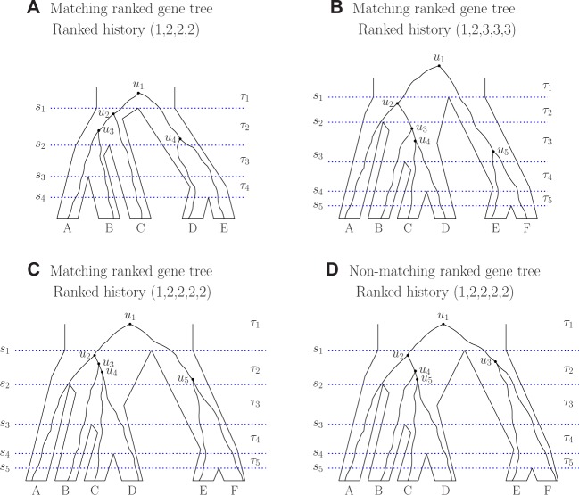
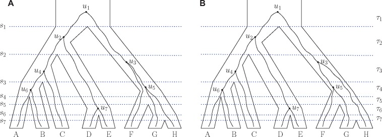
For a species tree with n labeled leaves, we assign ranks to the nodes according to their speciation order. Denote the time of the interior node of rank i (ith speciation) by s_i, $i=1,2,\dots ,n-1$. Time is zero for the leaves and increases going backward in time: $s_1>s_2>\dots >s_{n-1}$, where s₁ is the time of the root (fig. 1). For $i=2,3,\dots ,n-1$, denote the interval between the $(i-1)$th and ith speciation events by τ_i and its length by $t_i=s_{i-1}-s_i$.

Fig. 1.

Gene trees evolving on five-taxon and six-taxon species trees. (A) Five taxa. (B–D) Six taxa. The gene trees in (B)–(D) have the same unranked topology ((A,(B,(C, D))),(E, F)). Only the ranked gene tree topology in (D) does not match the ranked species tree topology. For each $i=1,2,\dots ,n-1,\hspace{0.17em}{s}_i\ge 0$ denotes the time of the ith speciation, τ_i represents the interval between the $(i-1)$th and ith speciation events, and u_i represents the ith coalescence (node with rank i) in the gene tree. Interval τ₁ has infinite length.

We write a ranked tree topology as a modified unranked tree topology using the Newick format, in which each clade is represented by a pair of parentheses, and we add a number after each clade to indicate its ranking. For example, the species tree in figure 1A can be written $({({(A,B)}_3,C)}_2,{(D,E)}_4)$. In the Newick format, we suppress the labeling of the root node, which has rank 1.

Let $\mathcal{G}$ be a ranked gene tree topology with the same labels for the leaves as species tree $\mathcal{T}$. Given a gene tree that evolves on a species tree $\mathcal{T}$, a “ranked history” can be defined as a nondecreasing sequence $x=(x_1,x_2,\dots ,x_{n-1})$, where for $i=1,2,\dots ,n-1$, x_i = j if the ith coalescence occurs in species tree interval τ_j (Degnan et al. 2012b). For example, in figure 1B, the ranked history of the gene tree is $(1,2,3,3,3)$. One coalescence occurs in the species tree interval τ₁, one in τ₂, and three in τ₃. We denote the probability under the coalescent model of a ranked gene tree topology with the particular ranked history x by $P(\mathcal{G},x|\mathcal{T})$.

If a gene tree and species tree have the same unranked topology, then we describe the unranked topologies as identical and refer to the unranked gene tree as “matching” the unranked species tree; otherwise, the gene tree topology is “nonmatching.” Similarly, we say the ranked gene tree matches the ranked species tree if, and only if, they have the same ranked topology. At times we will also be interested in cases where a ranked gene tree has the same unranked topology as the species tree, meaning that if the ranks are ignored, the two trees are matching. Because the methods in this article involve only topologies of gene trees, the term “gene tree” will be used to refer to the topology of the gene tree (without branch lengths) unless otherwise noted. Rooted labeled unranked or ranked gene tree topologies that are more probable than the labeled unranked or ranked gene tree topology matching the species tree are called anomalous gene trees and are termed AGTs and ARGTs, respectively. Species trees that have unranked or ranked anomalous gene trees are said to be in the unranked or ranked anomaly zone, respectively.

Results

We computed probabilities of ranked and unranked gene trees for species trees with five to eight taxa to find a subset of speciation interval length space in which a species tree has both anomalous unranked (AGTs) and ranked (ARGTs) gene trees. For plots comparing unrooted and unranked anomaly zones, see Degnan (2013).

Five Taxa

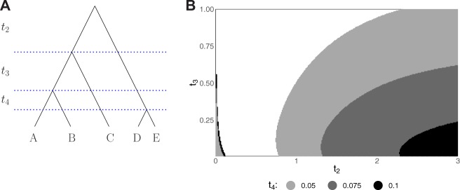
Figure 2A depicts a five-taxon species tree with interval lengths t₂, t₃, and t₄. The ranked topology shown is the only five-taxon species tree topology that possesses ARGTs. For fixed values of $t_4=0.05,0.075,0.1$, we computed the probabilities of all 105 unranked and all 180 ranked gene tree topologies on a grid with $t_2\in [0.01,3]$ and $t_3\in [0.01,1]$. The anomaly zones were identified by finding the set of values of t₂, t₃, and t₄ for which at least one nonmatching unranked or ranked gene tree topology has probability exceeding the probability of the corresponding matching gene tree topology.

Fig. 2.

Five-taxon anomaly zones. (A) The only ranked five-taxon species tree topology that produces ARGTs. The same species tree, with a gene tree evolving inside, is shown in figure 1A. (B) Slices of the unranked (on the left side) and ranked (on the right side) anomaly zones for the topology in (A). For fixed values of t₄, each shaded region represents pairs of speciation interval lengths (t₂, t₃) for which the most probable unranked (ranked) gene tree topology does not match the unranked (ranked) species tree topology. Each slice was generated by computing the probability distribution of gene tree topologies on a grid with $t_2\in [0.01,3]$ and $t_3\in [0.01,1]$, with increments of 0.01 for both variables. In the ranked case, the shaded region for a smaller t₄ contains the shaded region for a larger t₄. In the unranked case, the shaded region for a larger t₄ contains the shaded region for a smaller t₄.

Figure 2B depicts cross-sections of unranked and ranked anomaly zones for the five-taxon species tree in figure 2A. For values of t₂, t₃, and t₄ considered, we observe that the unranked and ranked anomaly zones do not overlap for five-taxon species trees. As t₄ becomes smaller, the ranked anomaly zone increases in size, whereas the size of the unranked anomaly zone decreases. Although for the values of t_i considered, we do not observe an overlap in unranked and ranked anomaly zones in the five-taxon case, these zones start to intersect for larger trees.

Six Taxa

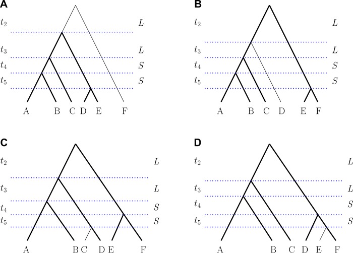
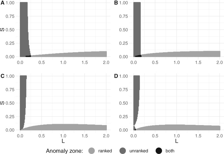
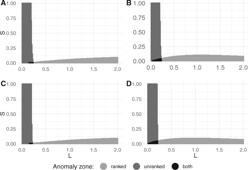
We next considered six-taxon trees. There exist six unlabeled tree shapes with six taxa. Excluding the caterpillar and pseudocaterpillar shapes, four of these, depicted in figure 3, give rise to both AGTs and ARGTs. Figure 4 shows 2D cross-sections of unranked and ranked anomaly zones for the six-taxon species tree topologies in figure 3. For ease of visualization, we consider only two different values, denoted by S and L, for the lengths of speciation intervals t_i. For each combination of $S\in [0.005,1]$ and $L\in [0.01,2]$, we computed the distributions of unranked and ranked gene tree topologies, and the presence of AGTs and ARGTs was then identified by comparing the analytical probabilities of the matching gene tree topology and the most probable nonmatching gene tree topology.

Fig. 3.

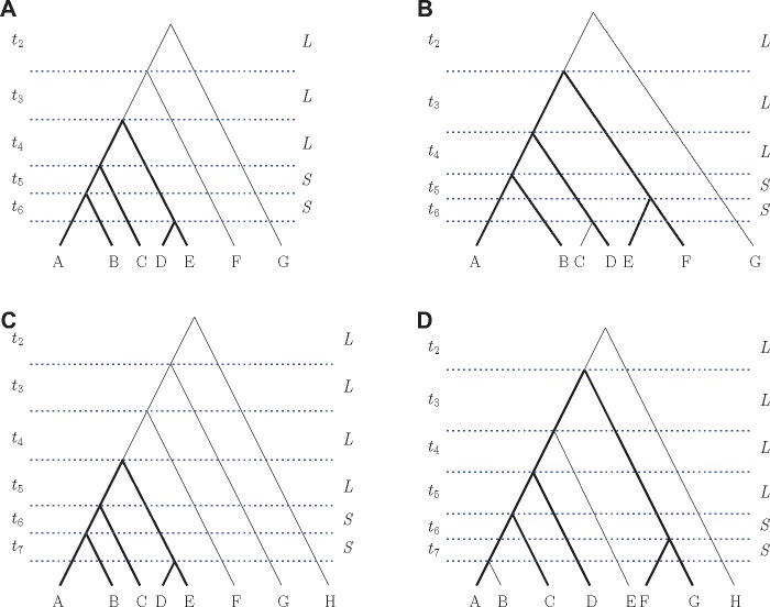
Representative labeled rankings of all six-taxon unlabeled species tree topologies, except the caterpillar and pseudocaterpillar. (A–D) Bold lines indicate a displayed five-taxon tree topology given in figure 2A. We set some lengths of the speciation intervals to be equal to aid in visualization and computation. Two values L and S, measured in coalescent units, are used as interval lengths. All values of L are equal to each other and all values of S are equal to each other. The figures are not drawn to scale.

Fig. 4.

2D cross-sections of unranked and ranked anomaly zones, each associated with a six-taxon species tree topology in the corresponding panel of figure 3. (A) Species tree in figure 3A. (B) Species tree in figure 3B. (C) Species tree in figure 3C. (D) Species tree in figure 3D. For each species tree topology, 200 values of $L\in [0.01,2]$ and 200 values of $S\in [0.005,1]$ were used to identify the existence of anomalous gene trees.

In the cases we examined, the two anomaly zones start to overlap only when lengths of the speciation intervals are short and not too distinct from each other. In particular, the intersection of anomaly zones is small for each topology, with the smallest overlap for the more balanced species tree topologies in figure 3C and D.

Seven and Eight Taxa

We next sought to examine scenarios with seven and eight taxa (fig. 5) to determine whether the interval-length cases giving rise to AGTs and ARGTs were similar to those seen in the case of six taxa.

Fig. 5.

Representative labeled rankings of two seven-taxon and two eight-taxon species tree topologies that produce anomalous gene trees. (A, B) Seven taxa. (C, D) Eight taxa. Bold lines indicate a displayed five-taxon tree topology given in figure 2A. We set some lengths of the speciation intervals to be equal to aid in visualization and computation. Two values L and S, measured in coalescent units, are used as interval lengths. All values of L are equal to each other and all values of S are equal to each other. The figures are not drawn to scale.

The seven- and eight-taxon species trees were chosen so that they produce both AGTs and ARGTs. To find such topologies, we used a “caterpillarization” technique of finding a short–short–long (SSL) pattern in three consecutive internal branches on a path from a tip to the root of the species tree, and setting all other branches to be long. In Degnan (2013), this technique was used to collapse taxa descended from long branches to be effectively a single taxon, making even a topologically balanced tree resemble a caterpillar when branch lengths are taken into account. More generally, the technique of setting some specific branches to be short and others to be long has been used frequently in identifying AGTs and ARGTs (Degnan and Rosenberg 2006; Degnan et al. 2009, 2012a, 2012b; Rosenberg 2013).

Here we use caterpillarization to make seven- and eight-taxon trees resemble the five-taxon ranked tree $({({(A,B)}_3,C)}_2,{(D,E)}_4)$, the only five-taxon ranked species tree that produces ARGTs. In particular, we consider cases in which a five-taxon species tree topology in figure 2A is contained inside the larger trees. This five-taxon tree appears with bold font in larger tree topologies (figs. 3 and 5). Because the five-taxon tree in figure 2A produces both AGTs and ARGTs, there exists a subset of branch lengths that makes larger trees also have AGTs and ARGTs simultaneously.

We observe a similar pattern in anomaly zones (fig. 6) for species tree topologies displayed in figures 3A, 5A, and 5C. Each of these topologies was obtained from the five-taxon topology in figure 2A by sequentially attaching an additional branch to the root. Under the restriction that speciation intervals have one of two lengths, S and L, anomaly zones behave somewhat similarly in the cases of $n=6,7,$ and 8. In particular, the species tree usually needs to have large values of L and small values of S to be in the ranked anomaly zone. However, the pattern is reversed for AGTs: To produce AGTs, L usually needs to be small whereas S may be relatively large.

Fig. 6.

2D cross-sections of unranked and ranked anomaly zones for associated seven- and eight-taxon species tree topologies in figure 5. (A) Species tree in figure 5A. (B) Species tree in figure 5B. (C) Species tree in figure 5C. (D) Species tree in figure 5D. For each species tree topology, 200 values of $L\in [0.01,2]$ and 200 values of $S\in [0.005,1]$ were used to identify the existence of anomalous gene trees.

Simulation Results

Next, to explore the probability that random species trees have AGTs and ARGTs, we performed simulations under a birth–death model. In particular, we simulated 5,000 species trees with $n=5,6,7,$ and 8-taxa under a constant-rate birth–death model using the TreeSim package in R (Stadler 2011). In this model, each species at each point in time has the same constant speciation (birth) rate λ and extinction (death) rate μ.

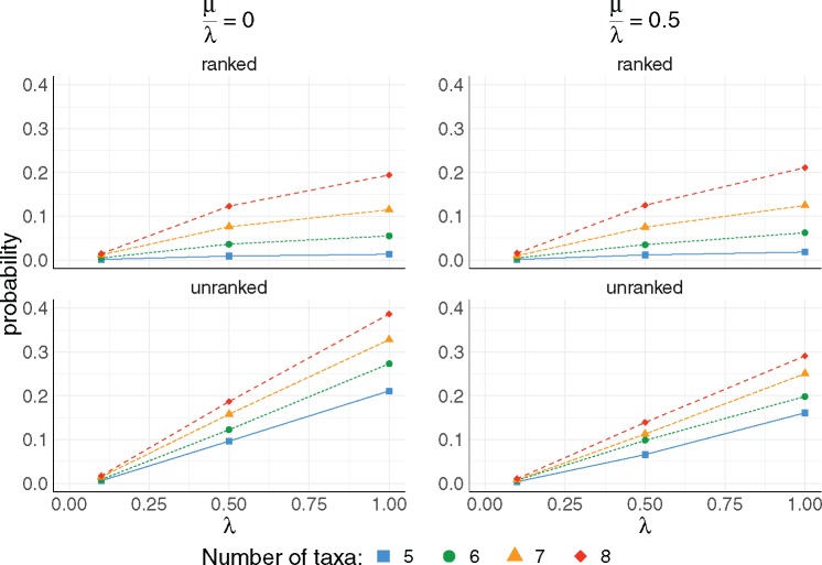
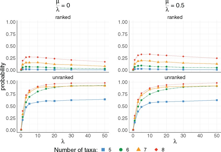
Figure 7 shows probabilities of the species tree being in the unranked and ranked anomaly zones in relation to the number of taxa n, speciation rate λ, and extinction rate μ. For both types of trees, the probability of a species tree being in an anomaly zone increases with the number of taxa and with λ. For unranked trees, both results are intuitive: For increasing numbers of taxa, there are more possible ways to have consecutive short branches or intervals in a tree, a pattern typical of the unranked anomaly zone (Rosenberg 2013). Increasing λ reduces the average branch length, making consecutive short branches more likely.

Fig. 7.

The impact of the speciation rate parameter λ and the turnover rate $\mu /\lambda$ on the existence of unranked and ranked anomaly zones. For each value of $n=5,6,7,$ and 8 taxa, 5,000 species trees were simulated using a constant-rate birth–death process with rates $\lambda =0.1,0.5,1$ and $\mu /\lambda =0,0.5$. For each combination of $(n,\lambda ,\mu )$, the probability of the species tree being in the anomaly zone was computed from the 5,000 trials.

We observed a different effect of the turnover rate $\mu /\lambda$ on the probability of producing unranked and ranked anomalous gene trees. The probability has a decreasing trend for the unranked anomaly zones and an increasing trend for the ranked anomaly zone as turnover rate increases. On average, branch lengths are longer as μ increases. In particular, a branch length near the root becomes longer, decreasing the probabilities of AGTs but increasing the probabilities of ARGTs.

We calculated the probabilities of ranked and unranked anomaly zones for specific five- and six-taxon tree topologies ($\lambda =0.1,0.5,1$, μ = 0, 5,000 replicates) to investigate the frequency with which the different tree shapes give rise to AGTs and ARGTs. Under the Yule process, the probabilities of a caterpillar shape, pseudocaterpillar shape, and the unranked version of the tree shape depicted in figure 2A for the five-taxon case are 1/3, 1/6, and 1/2, respectively. The conditional probabilities of a species tree being in the unranked anomaly zone given the shape are 7.42%, 0.87%, and 2.15% for the three shapes, respectively. Because neither caterpillar nor pseudocaterpillar species trees can produce ARGTs, the conditional probabilities of a species tree being in the ranked anomaly zone given the shape are 0%, 0%, and 0.77% for the three shapes, respectively.

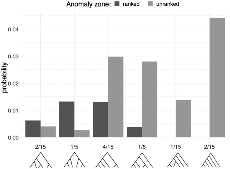
Figure 8 shows conditional probabilities of ranked and unranked anomaly zones for all possible six-taxon topologies when $\lambda =0.5$ and μ = 0. Under the Yule process, the unranked tree shapes have probabilities 2/15, 1/5, 4/15, 1/5, 1/15, and 2/15 from left to right. AGTs arise more often for the caterpillar shape, whereas ARGTs arise more often for the second and third shapes (from left to right). The full probability of anomalous gene trees can be calculated using the law of total probability.

Fig. 8.

Conditional probabilities of ranked and unranked anomaly zones given species tree shape for all possible six-taxon unlabeled, unranked species tree topologies. The exact probabilities of tree shapes under the Yule birth process are displayed on the x-axis. The results are based on 5,000 species trees simulated under the birth process with n = 6, $\lambda =0.5$, and μ = 0. Among the shapes with both AGTs and ARGTs, the third tree shape, with four taxa descended from one side of the root and two from the other, produces the largest combined frequency of AGTs and ARGTs. It is also the most probable shape under the birth process. Similar patterns occur for $\lambda =0.1$ and λ = 1 (not shown).

We also noticed that the probabilities of being in the unranked anomaly zone grow faster than those of the ranked anomaly zone as the speciation rate increases (fig. 9). For example, the probabilities that a species tree belongs to unranked and ranked anomaly zones are equal to 0.399 and 0.194, respectively, for n = 8, λ  =  1, and μ  =  0. For an eight-taxon species tree, with λ  =  10 and μ  =  0, these probabilities are equal to 0.909 and 0.267, respectively.

Fig. 9.

The impact of the speciation rate parameter $\lambda \in [0.1,50]$ and the turnover rate $\mu /\lambda =0$ and 0.5 on the existence of unranked and ranked anomaly zones. For each combination of $(n,\lambda ,\mu )$, the probability of the species tree being in the anomaly zone was computed from 5,000 species trees. Probabilities of the unranked anomaly zone appear to increase with λ, whereas probabilities of the ranked anomaly zone increase up to a certain value $\lambda \approx 5$ and then begin to decrease.

Discussion

The existence of anomalous gene trees poses challenges for inferring species trees from gene trees. We have studied AGTs and ARGTs for small trees, identifying cases in which a species tree possesses both types of anomalies (figs. 4 and 6). We studied how the parameters of the species tree (n, λ, μ) simulated under a constant-rate birth–death process can affect the probability that a species tree is in the anomaly zone. We have shown that often a species tree has lower probability to be in the ranked anomaly zone than in the unranked anomaly zone (figs. 7 and 9).

We also ran our simulations with larger values of λ, observing that the probabilities of unranked anomaly zones grow faster than those of ranked anomaly zones as the speciation rate increases (fig. 9). The probability of a species tree being in the ranked anomaly zone for n = 8 reaches a peak near 27.4% and begins to decrease for approximately $\lambda >5$. Probabilities of a species tree being in the unranked anomaly zone appear to increase with λ, but they are not approaching 1.

An intuitive reason that probabilities do not approach 1 for fixed n is that as λ increases, the probability increases that all coalescences occur more anciently than the root of the tree. This scenario does not always result in anomaly zones. For ranked trees, if the species tree is either a caterpillar or pseudocaterpillar, then there cannot be an ARGT, putting a limit on the probability that the species tree lies in the ranked anomaly zone when n is fixed. In the five-taxon case, ARGTs are more likely when interval τ₂, in which there are two populations (fig. 1A), is relatively large compared with other intervals. Increasing λ makes this condition less likely. For unranked species trees, if all coalescences occur above the root, then the species tree has AGTs if, and only if, the species tree does not have a maximally probable shape, where a maximally probable shape is one for which labeled topologies have the maximum number of possible rankings (Degnan and Rosenberg 2006). For example, for five taxa, the tree $(((A,B),C),(D,E))$ has three rankings. Thus, if the species tree has this topology and all internal branches have length 0, then no other gene tree shape can be anomalous for it. In this case, as $\lambda \to \infty$, an unranked labeled gene tree topology approaches probability $r/180$, where r is the number of rankings for the gene tree.

For six taxa, the unlabeled tree shape whose labeled topologies have the maximum number of rankings has four taxa descended from one side of the root and two from the other side, as shown in figure 3C, where the rooted subtrees on each side of the root themselves maximize the number of possible rankings. This scenario results in an unlabeled tree with eight rankings and 45 labelings. Because there are 2,700 ranked labeled topologies for n = 6 taxa, we therefore expect that as $\lambda \to \infty$, the probability of the species tree being in an unranked anomaly zone is at least $1-(45·8)/2,700=13/15$. This value occurs because labeled unranked trees with this maximally probable shape are tied in probability for being the most probable when all coalescences occur more anciently than the root; as $\lambda \to \infty$, the probability approaches 13/15 that the species tree does not have the maximally probable shape, and therefore is in an unranked anomaly zone.

More generally, let T_n be an unlabeled species tree shape with the maximum number of rankings. For large λ, the probability of the species tree with n leaves being in an unranked anomaly zone has a lower bound of

$$1-2^{n-1-\sigma (T_n)}\prod _{i=1}^{n-1}\hspace{0.17em}{[c_i(T_n)-1]}^{-1},$$ (1)

where $\sigma (T_n)$ is the number of balanced internal vertices of T_n and $c_i(T_n)$ is the number of descendant leaves of interior vertex i, including the root as an interior vertex. The lower bound given in equation (1) can be calculated as 1 minus the probability that the species tree under the Yule process has the shape that produces the largest number of rankings for a fixed labeling. For example, the lower bound for six-taxon species trees can be calculated as $1-2/15=13/15$. This lower bound in equation (1) underestimates the probability of being in an anomaly zone for large λ because even labeled species trees with the maximally probable shape can have AGTs for some sets of branch lengths. It can be shown that this lower bound approaches 1 as $n\to \infty$ (see Appendix for details).

In general, probabilities of both AGTs and ARGTs increase with the number of taxa. For example, going from five to eight taxa, the probability of an AGT approximately doubles, for both $\lambda =0.5$ and λ  =  1 at both levels of turnover (fig. 7). The probability of an ARGT increases by a factor of 10 to 15 going from five to eight taxa at $\lambda =0.5$ and λ  =  1 at both levels of turnover (fig. 7).

An open question from Degnan et al. (2012b) was whether the most probable ARGT could have a different “unranked” topology from that of the species tree. In that study, examples of ARGTs had different rankings from the species tree but the same unranked topology. Here, in our simulation with different combinations of values (n, λ, μ), we have not found any cases where the most probable ranked gene tree and the species tree have different unranked topologies. However, we found a few cases where a gene tree within one step by nearest-neighbor interchange—which has a different unranked topology from the species tree—has exactly the same ranked histories and probability as the ranked gene tree topology that matches the unranked species tree topology. For example, for a species tree given in figure 10, the two ranked gene trees in the figure have the same probabilities, because they have exactly the same values of $k_{i,j,z}$ and thus, the same values of ${\lambda }_{i,j}$ (see eq. 5 for details). The same result that at least one of the most probable ranked gene tree topologies must have the same unranked topology as the species tree was proved mathematically by Disanto et al. (2019). This result suggests that the “democratic vote” method used for ranked gene trees might be less misleading than in the unranked setting: If one takes the ranked gene tree (or gene trees, allowing for ties) that occurs most frequently in a large enough sample, then its unranked version is predicted to match the species tree, except possibly when another ranked gene tree is tied for being most probable.

Fig. 10.

Gene trees evolving on an eight-taxon species tree. (A) Ranked gene tree $({({({(A,B)}_6,C)}_4,{(D,E)}_7)}_2,{({(G,H)}_5,F)}_3)$ that shares the same unranked topology with that of the species tree. (B) Gene tree $({({({(A,B)}_6,C)}_4,{(D,E)}_7)}_2,{({(F,G)}_5,H)}_3)$ that has a different unranked topology from the species tree. Note that the ranked gene tree $({({({(A,B)}_6,C)}_4,{(D,E)}_7)}_2,{({(F,H)}_5,G)}_3)$ (not shown) has exactly the same probability as gene trees in (A) and (B) for the species tree depicted. For each $i=1,2,\dots ,7,\hspace{0.17em}{s}_i\ge 0$ denotes the time of the ith speciation, τ_i represents the interval between the $(i-1)$th and ith speciation events, t_i ($t_i=s_{i-1}-s_i,\hspace{0.17em}2\le i\le 7$) represents the length of interval τ_i, and u_i represents the ith coalescence (node with rank i) in the gene tree. The species tree has ranked topology $({({({(A,B)}_4,C)}_3,{(D,E)}_6)}_2,{({(G,H)}_7,F)}_5)$. For the species tree values $t_i=(0.29,0.006,0.041,0.001,0.022,0.001),\hspace{0.17em}i=2,3,\dots ,7$, the ranked gene trees in (A) and (B) are the most probable ranked gene trees, with probability $1.72404\times {10}^{-5}$.

Materials and Methods

Calculating the Probability of a Ranked Gene Tree Topology

General Formula

The probability of the ranked gene tree $P(\mathcal{G}|\mathcal{T})$ can be computed as a sum over all ranked histories. Denote the probability in interval τ_i for a particular ranked history x by $P({\mathcal{G}}_{{\tau }_i},x|T)$. The probability of a ranked gene tree topology $\mathcal{G}$ with ranked history set $\mathcal{Y}$ given a species tree $\mathcal{T}$ can be written

$$P\left(\mathcal{G}|\mathcal{T}\right)=\sum _{x\in \mathcal{Y}}{H}_{{\ell }_1}(x)\prod _{i=2}^{n-1}P({\mathcal{G}}_{{\tau }_i},x|\mathcal{T}),$$ (2)

where $H_{{\ell }_1}(x)$ is the probability that the coalescences above the root appear in the order that follows the ranked gene tree (Stadler and Degnan 2012). If the number of lineages above the root is ${\ell }_1$, then (Rosenberg 2006)

$$H_{{\ell }_1}(x)=\frac{2^{{\ell }_1-1}}{{\ell }_1!({\ell }_1-1)!}.$$ (3)

Denote the number of lineages available for coalescence in population z just after (going forward in time) the jth coalescence in interval τ_i by $k_{i,j,z}$. The probability that $\ell$ lineages fail to coalesce in a time interval of length t_i is ${\mathrm{e}}^{-\left(\begin{array}{c}\ell \\ 2\end{array}\right)t_i}$. Hence, the waiting time until the next coalescent event (going backward in time) has rate ${\lambda }_{i,j}=\sum _{z=1}^i\left(\begin{array}{c}{k}_{i,j,z}\\ 2\end{array}\right)$. The density for the coalescent events in the interval τ_i is (Degnan et al. 2012b)

$$f_i(v_0,v_1,\dots ,v_{m_i})=\text{exp}\hspace{0.17em}\left(-\sum _{j=0}^{m_i}{\lambda }_{i,j}{v}_j\right),$$ (4)

where v_j is the time between the jth and $(j+1)$st coalescent events, with v₀ being the time between $s_{i-1}$ and the least recent coalescent event in τ_i and with $v_{m_i}$ being the time between s_i and coalescent event m_i.

For example, consider the second speciation interval τ₂ for the species tree in figure 1A. Here, v₀ is the time between s₁ and the least recent coalescent event u₂ in interval τ₂. Similarly, v₁ is the time between u₂ and u₃, v₂ is the time between u₃ and u₄, and $v_{m_i}=v_3$ is the time between u₄ and s₂. Using the fact that the sum of exponential random variables with different rates λ_i has a hypoexponential distribution, equation (4) can be written as follows (Stadler and Degnan 2012):

$$P\left({\mathcal{G}}_{{\tau }_i},x|\mathcal{T}\right)={\int }_v{f}_i(v_0,\dots ,v_{m_i})\mathrm{d}v=\sum _{j=0}^{m_i}\frac{{\mathrm{e}}^{-{\lambda }_{i,j}(s_{i-1}-s_i)}}{\prod _{k=0,k\ne j}^{m_i}({\lambda }_{i,k}-{\lambda }_{i,j})}.$$ (5)

Examples

Consider a species tree $\mathcal{T}$ and gene tree with matching ranked topology $({(A,{(B,{(C,D)}_4)}_3)}_2,{(E,F)}_5)$ (fig. 1C). We now calculate the probability of the ranked history $(1,2,2,2,2)$ in interval τ₂. Because four coalescences occur in interval τ₂, $m_2=4$ and $k_{2,j,z}$ is defined for $j=0,1,2,3,4$ and z = 1, 2. We have $k_{2,j,1}=(1,2,3,4,4)$ for $j=0,1,\dots ,4$ and $k_{2,j,2}=(1,1,1,1,2)$ for $j=0,1,\dots ,4.$ Using ${\lambda }_{2,j}=\sum _{z=1}^2\left(\begin{array}{c}{k}_{2,j,z}\\ 2\end{array}\right)$, we have ${\lambda }_{2,j}=(0,1,3,6,7),$ for $j=0,1,\dots ,4.$ Thus, equation (5) evaluates to

$$P\left({\mathcal{G}}_{{\tau }_2},(1,2,2,2,2)|\mathcal{T}\right)=\sum _{j=0}^4\frac{{\mathrm{e}}^{-{\lambda }_{2,j}{t}_2}}{\prod _{k=0,k\ne j}^4({\lambda }_{2,k}-{\lambda }_{2,j})}=\frac{1}{126}-\frac{{\mathrm{e}}^{-t_2}}{60}+\frac{{\mathrm{e}}^{-3t_2}}{72}-\frac{{\mathrm{e}}^{-6t_2}}{90}+\frac{{\mathrm{e}}^{-7t_2}}{168},$$

where $t_2=s_1-s_2$ is the length of interval τ₂.

Similarly, we can compute the probabilities in intervals τ₃, τ₄, τ₅. Given that the probability for the coalescence of ${\ell }_1=2$ lineages above the root appearing in the right order is $H_2=1$ (eq. 3), the probability of the ranked history $(1,2,2,2,2)$ is equal to

$$\begin{array}{c}P\left(\mathcal{G},(1,2,2,2,2)|\mathcal{T}\right)=H_2(x)·\prod _{i=2}^{5}P\left({\mathcal{G}}_{{\tau }_i},(1,2,2,2,2)|\mathcal{T}\right)\\ =\left(\frac{1}{126}-\frac{{\mathrm{e}}^{-t_2}}{60}+\frac{{\mathrm{e}}^{-3t_2}}{72}-\frac{{\mathrm{e}}^{-6t_2}}{90}+\frac{{\mathrm{e}}^{-7t_2}}{168}\right)·{\mathrm{e}}^{-4t_3-2t_4-t_5},\end{array}$$ (6)

where $t_i=s_{i-1}-s_i.$

Now consider a species tree $\mathcal{T}$ and gene tree with nonmatching ranked topology $({(A,{(B,{(C,D)}_5)}_4)}_2,{(E,F)}_3)$ (fig. 1D). The values of $k_{i,j,z}$ in interval τ₂ are

$$k_{2,j,1}=(1,2,2,3,4),\hspace{0.17em}\hspace{0.17em}\hspace{0.17em}j=0,1,\dots ,4;\hspace{0.17em}\hspace{0.17em}{k}_{2,j,2}=(1,1,2,2,2),\hspace{0.17em}\hspace{0.17em}\hspace{0.17em}j=0,1,\dots ,4.$$

Thus, ${\lambda }_{2,j}=(0,1,2,4,7)$ for $j=0,1,\dots ,4$, and the probability of the nonmatching ranked gene tree for the ranked history $(1,2,2,2,2)$ is

$$\begin{array}{c}P\left(\mathcal{G},(1,2,2,2,2)|\mathcal{T}\right)=H_2(x)·\prod _{i=2}^{5}P\left({\mathcal{G}}_{{\tau }_i},(1,2,2,2,2)|\mathcal{T}\right)\\ =\left(\frac{1}{56}-\frac{{\mathrm{e}}^{-t_2}}{18}+\frac{{\mathrm{e}}^{-2t_2}}{20}-\frac{{\mathrm{e}}^{-4t_2}}{72}+\frac{{\mathrm{e}}^{-7t_2}}{630}\right)·{\mathrm{e}}^{-4t_3-2t_4-t_5}.\end{array}$$ (7)

Following equations (6) and (7), the limiting probabilities for the matching and nonmatching ranked gene tree topologies for the ranked history $(1,2,2,2,2)$ when $t_2\to \infty$ and $t_3,t_4,t_5\to 0$ are $\frac{1}{126}$ and $\frac{1}{56}$, respectively. Thus, the ranked history $(1,2,2,2,2)$ is more probable for the nonmatching ranked gene tree topology than for the matching ranked history when $t_2\to \infty$ and $t_3,t_4,t_5\to 0$. For sufficiently large t₂ and sufficiently small $t_3,t_4,t_5$, most of the probability of the ranked gene tree topology is concentrated on this ranked history, making the probabilities of the other ranked histories close to 0. Thus, the most probable ranked gene tree topology becomes discordant from the ranked species tree topology, forcing the species tree into the ranked anomaly zone.

PRANC Software

We implemented the program PRANC, which can analytically compute the probabilities of ranked gene trees given a species tree in Newick format, following equation (2). The program has an option to compute the probability of an unranked gene tree by summing the probabilities of all ranked gene trees that share the corresponding unranked topology. We improved the numerical results by adding the probabilities of the ranked histories in ascending order, enabling the smallest-magnitude values to accumulate before interacting with larger-magnitude values. In addition, PRANC has an option to output symbolic probabilities followed by ranked histories (https://github.com/anastasiiakim/PRANC):

$$\mathtt{pranc} -\mathtt{rprob}<\mathtt{species}-\mathtt{tree}-\mathtt{file}-\mathtt{name}><\mathtt{ranked}-\mathtt{gene}-\mathtt{tree}-\mathtt{file}-\mathtt{name}>$$

$$\mathtt{pranc} -\mathtt{uprob}<\mathtt{species}-\mathtt{tree}-\mathtt{file}-\mathtt{name}><\mathtt{unranked}-\mathtt{gene}-\mathtt{tree}-\mathtt{file}-\mathtt{name}>$$

$$\mathtt{pranc} -\mathtt{sym}<\mathtt{species}-\mathtt{tree}-\mathtt{file}-\mathtt{name}><\mathtt{ranked}-\mathtt{gene}-\mathtt{tree}-\mathtt{file}-\mathtt{name}>$$

PRANC also can output the “democratic vote” ranked or unranked tree topology. Using the following code, the program outputs two files: one with ranked or unranked topologies for each tree, and another with unique topologies and their frequencies,

$$\mathtt{pranc}-\mathtt{rtopo}<\mathtt{input}-\mathtt{file}-\mathtt{name}>$$

$$\mathtt{pranc}-\mathtt{utopo}<\mathtt{input}-\mathtt{file}-\mathtt{name}>$$

Simulations

We simulated species phylogenies under a constant-rate birth–death model. In this model, each species is equally likely to be the next to speciate. Each tree branch gives birth to a new branch at rate λ. Lineages can also go extinct at rate μ.

Because the length of a randomly selected interior branch in a Yule (rate λ) tree on n leaves is exponentially distributed with rate $2\lambda$ (Stadler and Steel 2012), for $\lambda =0.1$ and λ = 1, a species tree has a mean branch length of $1/(2·0.1)=5$ and $1/(2·1)=0.5$, respectively. We note that if all branch lengths were 0.5 coalescent units, then the species trees in the simulations would be outside of the unranked anomaly zone. A value of 0.5 coalescent units for an internal branch means that two lineages have a probability of $1-\text{exp}(-0.5)\approx 39\%$ of coalescing within that branch, whereas for 5 coalescent units, the probability of coalescence exceeds 99%. Values of λ near 0.5 are chosen to be reasonably plausible for hominid evolution (Stadler et al. 2016). The range of $\lambda =0.1$ to λ = 1 thus gives a range of low to moderate levels of incomplete lineage sorting that are plausibly consistent with empirical studies.

We let the speciation rate λ take the values of $0.1,0.5,$ and 1 and choose the extinction rate μ to depend on λ such that the turnover rate $\mu /\lambda$ is 0 or 0.5. Values of $(n,\lambda ,\mu )$ were chosen to examine the effect of the species tree parameters on the existence of anomalous gene trees. For each combination $(n,\lambda ,\mu )$, the distributions of unranked and ranked gene tree topologies were computed analytically for each simulated species tree. The probabilities of all possible unranked and ranked topologies were computed using “hybrid-coal” (Zhu and Degnan 2017) and PRANC, respectively, conditional on a species tree generated under a constant-rate birth–death model with parameters $(n,\lambda ,\mu )$. The presence of anomalous gene trees was then identified by comparing the analytical probabilities of the matching gene tree topology and the most probable nonmatching gene tree topology.

Appendix

Here we prove the lower bound in equation (1) of the probability of the species tree with n leaves being in an unranked anomaly zone for large λ, and we show that this lower bound approaches 1 as $n\to \infty$ and $\lambda \to \infty$.

Let T_n be a labeled species tree whose unlabeled shape maximizes the number of rankings of its associated labeled topologies. For large λ, the probability of the species tree with n leaves being in an unranked anomaly zone has a lower bound of

$$1-\frac{N_{\mathrm{R}}·R}{N_{\mathrm{T}}},$$ (8)

where N_R is the number of ways to label the unranked unlabeled tree with the maximum number of rankings, R is the number of rankings, and N_T is the number of ranked topologies for an n-taxon labeled tree.

A given unlabeled tree topology has $R=(n-1)!/{\prod }_{i=1}^{n-1}(c_i-1)$ rankings, where c_i is the number of descendant leaves of interior vertex i, including the root as an interior vertex (Steel 2016, p. 46). There are $N_{\mathrm{R}}=n!2^{-\sigma }$ ways to label the tree with the maximum number of rankings, where σ is the number of balanced internal vertices (Steel 2016). Because the number of ranked topologies for an n-taxon tree is $N_{\mathrm{T}}=\prod _{i=2}^n\left(\begin{array}{c}i\\ 2\end{array}\right)=n!(n-1)!/2^{n-1}$ (Brown 1994; Steel 2016), equation (8) leads to the following expression:

$$1-\frac{n!2^{-\sigma (T_n)}·(n-1)!\prod _{i=1}^{n-1}\hspace{0.17em}{[c_i(T_n)-1]}^{-1}}{n!(n-1)!/2^{n-1}}=1-\frac{2^{n-1-\sigma (T_n)}}{(n-1)\prod _{i=2}^{n-1}\hspace{0.17em}[c_i(T_n)-1]},$$ (9)

equivalent to the expression (1).

An n-taxon labeled species tree T_n with the maximum number of rankings has $2^{1+\lfloor {\hspace{0.17em}\text{log}\hspace{0.17em}}_2[(n-1)/3]\rfloor }$ taxa descended from one side of the root and $n-2^{1+\lfloor {\hspace{0.17em}\text{log}\hspace{0.17em}}_2[(n-1)/3]\rfloor }$ from the other side (Harding 1971, 1974; Hammersley and Grimmett 1974) (table 1). For an n-taxon tree, n must be between two powers of 2. Let $k\ge 0$ be an integer with $2^{k+1}<n\le 2^{k+2}$. For a tree with the maximum number of rankings, one of the subtrees descended from T_n has at most $2^{k+1}$ leaves and has the number of leaves a power of 2. In particular, T_n with $2^{k+1}<n\le 2^{k+2}$ leaves has $2^k\le 2^{1+\lfloor {\hspace{0.17em}\text{log}\hspace{0.17em}}_2[(n-1)/3]\rfloor }\le 2^{k+1}$ taxa descended from one side of the root and $2^k<n-2^{1+\lfloor {\hspace{0.17em}\text{log}\hspace{0.17em}}_2[(n-1)/3]\rfloor }\le 2^{k+1}$ from the other side (table 1 and fig. 11). The tree rooted on each side of the root of T_n itself maximizes the number of possible rankings for all labeled trees with the same number of leaves.

Fig. 11.

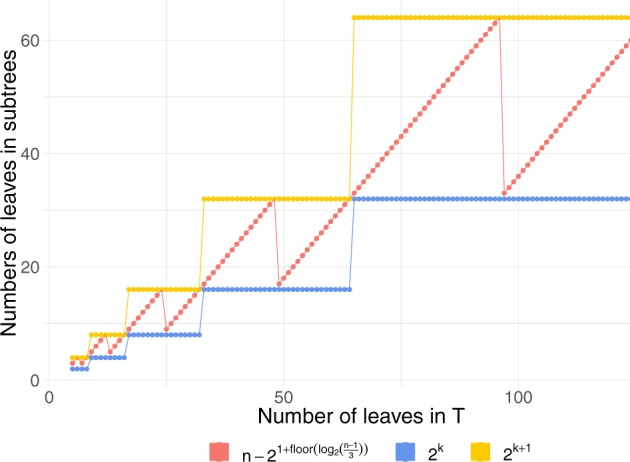
The values of $n-2^{1+\lfloor {\hspace{0.17em}\text{log}\hspace{0.17em}}_2[(n-1)/3]\rfloor },\hspace{0.17em}{2}^k$, and $2^{k+1}$ for a tree with $2^{k+1}<n\le 2^{k+2}$ taxa. The tree with the maximum number of rankings has $2^k\le 2^{1+\lfloor {\hspace{0.17em}\text{log}\hspace{0.17em}}_2[(n-1)/3]\rfloor }\le 2^{k+1}$ taxa descended from one side of the root and $2^k<n-2^{1+\lfloor {\hspace{0.17em}\text{log}\hspace{0.17em}}_2[(n-1)/3]\rfloor }\le 2^{k+1}$ from the other side.

Table 1.

The n-Taxon Species Trees with the Maximum Number of Rankings for a Labeled Topology.

n	$(\ell ,r)$	n	$(\ell ,r)$	n	$(\ell ,r)$	n	$(\ell ,r)$
2	(1, 1)	18	(10, 8)	34	(18, 16)	50	(32, 18)
3	(2, 1)	19	(11, 8)	35	(19, 16)	51	(32, 19)
4	(2, 2)	20	(12, 8)	36	(20, 16)	52	(32, 20)
5	(3, 2)	21	(13, 8)	37	(21, 16)	53	(32, 21)
6	(4, 2)	22	(14, 8)	38	(22, 16)	54	(32, 22)
7	(4, 3)	23	(15, 8)	39	(23, 16)	55	(32, 23)
8	(4, 4)	24	(16, 8)	40	(24, 16)	56	(32, 24)
9	(5, 4)	25	(16, 9)	41	(25, 16)	57	(32, 25)
10	(6, 4)	26	(16, 10)	42	(26, 16)	58	(32, 26)
11	(7, 4)	27	(16, 11)	43	(27, 16)	59	(32, 27)
12	(8, 4)	28	(16, 12)	44	(28, 16)	60	(32, 28)
13	(8, 5)	29	(16, 13)	45	(29, 16)	61	(32, 29)
14	(8, 6)	30	(16, 14)	46	(30, 16)	62	(32, 30)
15	(8, 7)	31	(16, 15)	47	(31, 16)	63	(32, 31)
16	(8, 8)	32	(16, 16)	48	(32, 16)	64	(32, 32)
17	(9, 8)	33	(17, 16)	49	(32, 17)	65	(33, 32)

Note.—The tree with the maximum number of rankings splits into (left, right) subtrees with $(\ell ,r)$ leaves. The n-taxon species tree with the maximum number of rankings T_n has $2^{1+\lfloor {\hspace{0.17em}\text{log}\hspace{0.17em}}_2[(n-1)/3]\rfloor }$ taxa descended from one side of the root and $n-2^{1+\lfloor {\hspace{0.17em}\text{log}\hspace{0.17em}}_2[(n-1)/3]\rfloor }$ from the other side.

To prove that the lower bound approaches 1 as $n\to \infty$, we need to show that in equation (9), ${\prod }_{i=2}^{n-1}\hspace{0.17em}{[c_i(T_n)-1]}^{-1}\to 0$ and $2^{n-1-\sigma (T_n)}{(n-1)}^{-1}\le 1$ as $n\to \infty$. We consider three cases: 1) $n=2^{k+2}$, 2) n odd, and 3) n even and $n\ne 2^{k+2}$.

Consider a case with $n=2^{k+2},\hspace{0.17em}k=0,1,\dots$. A completely balanced symmetric shape is the shape with the maximum number of rankings, with $\sigma (T_n)=n-1$. Thus, for $n=2^{k+2}$, equation (9) can be written as follows:

$$1-\prod _{i=1}^{k+1}{(2^{k-i+3}-1)}^{-2^{i-1}}.$$ (10)

The product in equation (10) is the inverse product of the numbers of descendant leaves of all interior vertices, including the root as an interior vertex. That the lower bound for $n=2^{k+2}$ approaches 1 as $k\to \infty$ is proven by Lemma 1.

Lemma 1. —

Let $c_i(T_n)$ be the number of descendant leaves of interior vertex i of a tree T_n, excluding the root. Then ${\prod }_{i=2}^{n-1}\hspace{0.17em}{[c_i(T_n)-1]}^{-1}\to 0$ as $n\to \infty$.

Proof. Define $c_i^{*}$ as

$$c_i^{*}=\{\begin{array}{cc}2,\hfill & \text{if}\hspace{0.17em}\mathrm{i} \text{is} \mathrm{a} \text{cherry},\hfill \\ 3,\hfill & \text{otherwise}.\hfill \end{array}$$

The maximum number of cherries of an n-taxon tree is at most $n/2$. Hence,

$$\prod _{i=2}^{n-1}\hspace{0.17em}{[c_i(T_n)-1]}^{-1}\le \prod _{i=2}^{n-1}\hspace{0.17em}{[c_i^{*}(T_n)-1]}^{-1}\le 2^{-(n-2-n/2)}=2^{-n/2+2},$$

where $n-2-n/2$ is the number of internal nodes excluding the root minus the maximum number of cherries. This quantity approaches 0 as $n\to \infty$, completing the proof. □

For the other two cases, we use a series of lemmas. Table 2 depicts the results of Lemmas 2 and 3.

Table 2.

The Number of Balanced Internal Vertices $\sigma (T_n)$ in n-Taxon Species Trees with the Maximum Number of Rankings for a Labeled Topology.

n Even			n Odd
n	$\sigma (T_n)$	$n-1-\sigma (T_n)$	n	$\sigma (T_n)$	$n-1-\sigma (T_n)$
2	1	0	3	1	1
4	3	0	5	2	2
6	4	1	7	4	2
8	7	0	9	5	3
10	7	2	11	7	3
12	10	1	13	9	3
14	11	2	15	11	3
16	15	0	17	12	4
18	14	3	19	14	4
20	17	2	21	16	4
22	18	3	23	18	4
24	22	1	25	20	4
26	22	3	27	22	4
28	25	2	29	24	4
30	26	3	31	26	4
32	31	0	33	27	5
34	29	4	35	29	5
36	32	3	37	31	5
38	33	4	39	33	5
40	37	2	41	35	5
42	37	4	43	37	5
44	40	3	45	39	5
46	41	4	47	41	5
48	46	1	49	43	5
50	45	4	51	45	5
52	48	3	53	47	5
54	49	4	55	49	5
56	53	2	57	51	5
58	53	4	59	53	5
60	56	3	61	55	5
62	57	4	63	57	5
64	63	0	65	58	6

Note.—For even n, $\sigma (T_n)\ge n-k-1$ (Lemma 3). For completely balanced and symmetric $n=2^{k+2}$-taxon trees, $\sigma (T_n)=n-1$. For $n=3·2^{\lfloor {\hspace{0.17em}\text{log}\hspace{0.17em}}_2(n)-1\rfloor }$-taxon trees, $\sigma (T_n)=n-2$. For odd n, the number of balanced internal vertices is $\sigma (T_n)=n-1-\lfloor {\hspace{0.17em}\text{log}\hspace{0.17em}}_{2}n\rfloor$ (Lemma 2).

Lemma 2: —

Let $\sigma (T_n)$ be the number of balanced internal vertices in T_n, the tree with the maximal number of rankings. Then, $\sigma (T_n)=n-k-1$ when n is odd and $2^k<n<2^{k+1},k\ge 1$.

Proof. Let C(k) be the statement that for odd n and $2^k<n<2^{k+1},\hspace{0.17em}\sigma (T_n)=n-k-1$. C(k) is true for k = 1 as 3-taxon trees have one balanced internal vertex. Now we show that if C(k) is true, then $C(k+1)$ is true for any $k\ge 1$.

We need to show that for odd n, $2^{k+1}<n<2^{k+2}$, the number of balanced internal vertices is $\sigma (T_n)=n-(k+1)-1=n-k-2$.

Among trees with $2^{k+1}<n<2^{k+2}$ leaves, let T_n be a tree with the maximal number of rankings. Let $\ell (T_{\mathrm{L}})$ and $\ell (T_{\mathrm{R}})$ be the numbers of leaves in the trees rooted at the left and right immediate descendants of the root, respectively. Without loss of generality, let $\ell (T_{\mathrm{L}})=2^{1+\lfloor {\hspace{0.17em}\text{log}\hspace{0.17em}}_2[(n-1)/3]\rfloor }$ and $\ell (T_{\mathrm{R}})=n-2^{1+\lfloor {\hspace{0.17em}\text{log}\hspace{0.17em}}_2[(n-1)/3]\rfloor }$.

T _L is a completely balanced symmetric tree, $\sigma (T_{\mathrm{L}})=2^{1+\lfloor {\hspace{0.17em}\text{log}\hspace{0.17em}}_2[(n-1)/3]\rfloor }-1$. Because n is odd, T_R has an odd number of leaves with $2^k<n-2^{1+\lfloor {\hspace{0.17em}\text{log}\hspace{0.17em}}_2[(n-1)/3]\rfloor }<2^{k+1}$ for $2^{k+1}<n<2^{k+2}$ (fig. 11).

Now, using an induction assumption that C(k) is true, $\sigma (T_n)=\sigma (T_{\mathrm{L}})+\sigma (T_{\mathrm{R}})=2^{1+\lfloor {\hspace{0.17em}\text{log}\hspace{0.17em}}_2[(n-1)/3]\rfloor }-1+(n-2^{1+\lfloor {\hspace{0.17em}\text{log}\hspace{0.17em}}_2[(n-1)/3]\rfloor }-k-1)=n-k-2$. □

Lemma 3. —

Let $\sigma (T_n)$ be the number of balanced internal vertices in T_n, the tree with the maximal number of rankings. Then $\sigma (T_n)\ge n-k-1$ when n is even and $2^k<n\le 2^{k+1},\hspace{0.17em}k\ge 0$.

Proof. Let C(k) be the statement that for even n and $2^k<n\le 2^{k+1},\hspace{0.17em}\sigma (T_n)\ge n-k-1$. Obviously, C(k) is true for k = 0 as 2-taxon trees have one balanced internal vertex ($\sigma (T_2)\ge 1$). Now we show that if C(k) is true, then $C(k+1)$ is true for any $k\ge 0$.

We need to show that for even n, $2^{k+1}<n\le 2^{k+2}$, the number of balanced internal vertices is $\sigma (T_n)\ge n-(k+1)-1=n-k-2$.

Among trees with $2^{k+1}<n\le 2^{k+2}$ leaves, let T_n be a tree with the maximal number of rankings. Let $\ell (T_{\mathrm{L}})$ and $\ell (T_{\mathrm{R}})$ be the numbers of leaves in the trees rooted at the left and right immediate descendants of the root, respectively. Without loss of generality, let $\ell (T_{\mathrm{L}})=2^{1+\lfloor {\hspace{0.17em}\text{log}\hspace{0.17em}}_2[(n-1)/3]\rfloor }$ and $\ell (T_{\mathrm{R}})=n-2^{1+\lfloor {\hspace{0.17em}\text{log}\hspace{0.17em}}_2[(n-1)/3]\rfloor }$.

T _L is a completely balanced symmetric tree, $\sigma (T_{\mathrm{L}})=2^{1+\lfloor {\hspace{0.17em}\text{log}\hspace{0.17em}}_2[(n-1)/3]\rfloor }-1$. Because n is even, T_R has an even number of leaves with $2^k<n-2^{1+\lfloor {\hspace{0.17em}\text{log}\hspace{0.17em}}_2[(n-1)/3]\rfloor }\le 2^{k+1}$ for $2^{k+1}<n\le 2^{k+2}$ (fig. 11).

Now, using an induction assumption that C(k) is true, $\sigma (T_n)=\sigma (T_{\mathrm{L}})+\sigma (T_{\mathrm{R}})\ge 2^{1+\lfloor {\hspace{0.17em}\text{log}\hspace{0.17em}}_2[(n-1)/3]\rfloor }-1+(n-2^{1+\lfloor {\hspace{0.17em}\text{log}\hspace{0.17em}}_2[(n-1)/3]\rfloor }-k-1)=n-k-2$. □

Lemma 4. —

$2^{n-1-\sigma (T_n)}{(n-1)}^{-1}\le 1$ as $n\to \infty$.

Proof. From Lemmas 2 and 3, it follows that $\sigma (T_n)\ge n-k-1$ for $2^k<n\le 2^{k+1}$ and ${\hspace{0.17em}\text{log}\hspace{0.17em}}_2(n)-1\le k<{\hspace{0.17em}\text{log}\hspace{0.17em}}_2(n)$.

Consider two cases: $k={\hspace{0.17em}\text{log}\hspace{0.17em}}_2(n)-1$ and ${\hspace{0.17em}\text{log}\hspace{0.17em}}_2(n)-1<k<{\hspace{0.17em}\text{log}\hspace{0.17em}}_2(n)$. If $k={\hspace{0.17em}\text{log}\hspace{0.17em}}_2(n)-1$, then $\sigma (T_n)\ge n-{\hspace{0.17em}\text{log}\hspace{0.17em}}_2(n)$ and

$$2^{n-1-\sigma (T_n)}\le 2^{{\hspace{0.17em}\text{log}\hspace{0.17em}}_2(n)-1}=2^{{\hspace{0.17em}\text{log}\hspace{0.17em}}_2(n)}/2=n/2\le n-1.$$

From ${\hspace{0.17em}\text{log}\hspace{0.17em}}_2(n)-1<k<{\hspace{0.17em}\text{log}\hspace{0.17em}}_2(n)$ and the fact that k is an integer, $k=\lfloor {\hspace{0.17em}\text{log}\hspace{0.17em}}_2(n)\rfloor$ and $\sigma (T_n)\ge n-1-\lfloor {\hspace{0.17em}\text{log}\hspace{0.17em}}_2(n)\rfloor$. Then, as $n\to \infty$

$$2^{n-1-\sigma (T_n)}\le 2^{\lfloor {\hspace{0.17em}\text{log}\hspace{0.17em}}_2(n)\rfloor }\le 2^{{\hspace{0.17em}\text{log}\hspace{0.17em}}_2(n-1)}=n-1.$$

It follows that, as $n\to \infty$,

$$2^{n-1-\sigma (T_n)}{(n-1)}^{-1}\le (n-1)/(n-1)=1.$$

□

Theorem. The lower bound of the probability of the species tree with n leaves being in an unranked anomaly zone, as defined in equation (9), approaches 1 as $n\to \infty$ and $\lambda \to \infty$.

Proof. The result immediately follows by Lemmas 1 and 4 in equation (9). □

References

- Brown JKM. 1994. Probabilities of evolutionary trees. Syst Biol. 43(1):78–91. [Google Scholar]
- Castillo-Ramírez S, González V.. 2008. Factors affecting the concordance between orthologous gene trees and species tree in bacteria. BMC Evol Biol. 8(1):300.. [DOI] [PMC free article] [PubMed] [Google Scholar]
- Degnan JH. 2013. Anomalous unrooted gene trees. Syst Biol. 62(4):574–590. [DOI] [PubMed] [Google Scholar]
- Degnan JH, DeGiorgio M, Bryant D, Rosenberg NA.. 2009. Properties of consensus methods for inferring species trees from gene trees. Syst Biol. 58(1):35–54. [DOI] [PMC free article] [PubMed] [Google Scholar]
- Degnan JH, Rhodes JA.. 2015. There are no caterpillars in a wicked forest. Theor Popul Biol. 105:17–23. [DOI] [PubMed] [Google Scholar]
- Degnan JH, Rosenberg NA.. 2006. Discordance of species trees with their most likely gene trees. PLoS Genet. 2(5):e68. [DOI] [PMC free article] [PubMed] [Google Scholar]
- Degnan JH, Rosenberg NA, Stadler T.. 2012a. A characterization of the set of species trees that produce anomalous ranked gene trees. IEEE/ACM Trans Comput Biol Bioinform. 9(6):1558–1568. [DOI] [PubMed] [Google Scholar]
- Degnan JH, Rosenberg NA, Stadler T.. 2012b. The probability distribution of ranked gene trees on a species tree. Math Biosci. 235(1):45–55. [DOI] [PubMed] [Google Scholar]
- Degnan JH, Salter LA.. 2005. Gene tree distributions under the coalescent process. Evolution 59(1):24–37. [PubMed] [Google Scholar]
- Disanto F, Miglionico P, Narduzzi G.. 2019. On the unranked topology of maximally probable ranked gene tree topologies. J Math Biol. 79(4):1205–1225. [DOI] [PubMed] [Google Scholar]
- Disanto F, Rosenberg NA.. 2014. On the number of ranked species trees producing anomalous ranked gene trees. IEEE/ACM Trans Comput Biol Bioinform. 11(6):1229–1238. [DOI] [PubMed] [Google Scholar]
- Hammersley JM, Grimmett GR.. 1974. Maximal solutions of the generalized subadditive inequality. In: Harding EF, Kendall DG, editors. Stochastic geometry. New York: John Wiley and Sons. p. 270–285. [Google Scholar]
- Harding EF. 1971. The probabilities of rooted tree-shapes generated by random bifurcation. Adv Appl Probab. 3(1):44–77. [Google Scholar]
- Harding EF. 1974. The probabilities of the shapes of randomly bifurcating trees. In: Harding EF, Kendall DG, editors. Stochastic geometry. New York: John Wiley and Sons. p. 259–269. [Google Scholar]
- Linkem CW, Minin VN, Leache AD.. 2016. Detecting the anomaly zone in species trees and evidence for a misleading signal in higher-level skink phylogeny (Squamata: Scincidae). Syst Biol. 65(3):465–477. [DOI] [PMC free article] [PubMed] [Google Scholar]
- Meng C, Kubatko LS.. 2009. Detecting hybrid speciation in the presence of incomplete lineage sorting using gene tree incongruence: a model. Theor Popul Biol. 75(1):35–45. [DOI] [PubMed] [Google Scholar]
- Nei M. 1987. Molecular evolutionary genetics. New York: Columbia University Press. [Google Scholar]
- Pamilo P, Nei M.. 1988. Relationships between gene trees and species trees. Mol Biol Evol. 5(5):568–583. [DOI] [PubMed] [Google Scholar]
- Rosenberg NA. 2002. The probability of topological concordance of gene trees and species trees. Theor Popul Biol. 61(2):225–247. [DOI] [PubMed] [Google Scholar]
- Rosenberg NA. 2006. The mean and variance of the numbers of r-pronged nodes and r-caterpillars in Yule-generated genealogical trees. Ann Comb. 10(1):129–146. [Google Scholar]
- Rosenberg NA. 2007. Counting coalescent histories. J Comput Biol. 14(3):360–377. [DOI] [PubMed] [Google Scholar]
- Rosenberg NA. 2013. Discordance of species trees with their most likely gene trees: a unifying principle. Mol Biol Evol. 30(12):2709–2713. [DOI] [PMC free article] [PubMed] [Google Scholar]
- Rosenberg NA, Tao R.. 2008. Discordance of species trees with their most likely gene trees: the case of five taxa. Syst Biol. 57(1):131–140. [DOI] [PubMed] [Google Scholar]
- Shi C-M, Yang Z.. 2018. Coalescent-based analyses of genomic sequence data provide a robust resolution of phylogenetic relationships among major groups of gibbons. Mol Biol Evol. 35(1):159–179. [DOI] [PMC free article] [PubMed] [Google Scholar]
- Stadler T. 2011. Simulating trees on a fixed number of extant species. Syst Biol. 60(5):676–684. [DOI] [PubMed] [Google Scholar]
- Stadler T, Degnan JH.. 2012. A polynomial time algorithm for calculating the probability of a ranked gene tree given a species tree. Algorithms Mol Biol. 7(1):7. [DOI] [PMC free article] [PubMed] [Google Scholar]
- Stadler T, Degnan JH, Rosenberg NA.. 2016. Does gene tree discordance explain the mismatch between macroevolutionary models and empirical patterns of tree shape and branching times? Syst Biol. 65(4):628–639. [DOI] [PMC free article] [PubMed] [Google Scholar]
- Stadler T, Steel M.. 2012. Distribution of branch lengths and phylogenetic diversity under homogeneous speciation models. J Theor Biol. 297:33–40. [DOI] [PubMed] [Google Scholar]
- Steel M. 2016. Phylogeny: discrete and random processes in evolution. Philadelphia (PA): Society for Industrial and Applied Mathematics (SIAM; ). [Google Scholar]
- Takahata N. 1989. Gene genealogy in three related populations: consistency probability between gene and population trees. Genetics 122(4):957–966. [DOI] [PMC free article] [PubMed] [Google Scholar]
- Wu Y. 2012. Coalescent-based species tree inference from gene tree topologies under incomplete lineage sorting by maximum likelihood. Evolution 66(3):763–775. [DOI] [PubMed] [Google Scholar]
- Xu B, Yang Z.. 2016. Challenges in species tree estimation under the multispecies coalescent model. Genetics 204(4):1353–1368. [DOI] [PMC free article] [PubMed] [Google Scholar]
- Yu Y, Degnan JH, Nakhleh L.. 2012. The probability of a gene tree topology within a phylogenetic network with applications to hybridization detection. PLoS Genet 8(4):e1002660.. [DOI] [PMC free article] [PubMed] [Google Scholar]
- Zhaxybayeva O, Doolittle WF, Papke RT, Gogarten JP.. 2009. Intertwined evolutionary histories of marine Synechococcus and Prochlorococcus marinus. Genome Biol Evol. 1:325–339. [DOI] [PMC free article] [PubMed] [Google Scholar]
- Zhu J, Yu Y, Nakhleh L.. 2016. In the light of deep coalescence: revisiting trees within networks. BMC Bioinformatics 17(Suppl 14):415.. [DOI] [PMC free article] [PubMed] [Google Scholar]
- Zhu S, Degnan JH.. 2017. Displayed trees do not determine distinguishability under the network multispecies coalescent. Syst Biol. 66:283–298. [DOI] [PMC free article] [PubMed] [Google Scholar]