Abstract
We study the spreading of contagious diseases in a population of constant size using susceptible-infective-recovered (SIR) models described in terms of ordinary differential equations (ODEs) and probabilistic cellular automata (PCA). In the PCA model, each individual (represented by a cell in the lattice) is mainly locally connected to others. We investigate how the topological properties of the random network representing contacts among individuals influence the transient behavior and the permanent regime of the epidemiological system described by ODE and PCA. Our main conclusions are: (1) the basic reproduction number (commonly called ) related to a disease propagation in a population cannot be uniquely determined from some features of transient behavior of the infective group; (2) cannot be associated to a unique combination of clustering coefficient and average shortest path length characterizing the contact network. We discuss how these results can embarrass the specification of control strategies for combating disease propagations.
Keywords: Basic reproduction number, Epidemiology, Ordinary differential equations, Probabilistic cellular automata, Random networks, SIR model
1. Introduction
Models based on probabilistic cellular automata (PCA) have been employed for investigating the spreading of contagious diseases (e.g. Ahmed et al., 1998, Doran and Laffan, 2005, Fuentes and Kuperman, 1999, Monteiro et al., 2006a, Monteiro et al., 2007, Sirakoulis et al., 2000, Yakowitz et al., 1990). In these epidemiological studies, the population is divided in three groups, as in the classical SIR model proposed by Kermack and McKendrick in 1927 (e.g. Anderson and May, 1992, Murray, 2003): the group S represents the individuals that are susceptible and thus subjected to the infection; the group I is formed by the individuals that are infected and can transmit the disease for susceptible ones; and the group R is composed by the individuals that are recovered. Equivalences with models based on ordinary differential equations (ODEs) are explored in some works (e.g. Ahmed et al., 1998, Fuentes and Kuperman, 1999, Monteiro et al., 2006a, Monteiro et al., 2007), since ODE are a mean-field approximation for PCA if the three groups (S, I and R) are homogeneously distributed in space.
In PCA models, in order to represent an infection process with a short-range character, each cell in the lattice (usually corresponding to an individual in the population) interacts with two (e.g. Ahmed et al., 1998), four (e.g. Yakowitz et al., 1990) or eight surrounding neighbors (e.g. Doran and Laffan, 2005, Fuentes and Kuperman, 1999, Monteiro et al., 2006a, Monteiro et al., 2007, Sirakoulis et al., 2000). In fact, disease-causing contacts form a connection network among individuals and the assumption of a topology in which the couplings are local and regular is just a first approximation. When long-range interactions are also taken into account, random coupling topologies are frequently employed (e.g. Boccaletti et al., 2006, Kleczkowski and Grenfell, 1999, Newmann, 2002) and relations among topological properties and features of the epidemiological dynamics (for instance, the number of infective individuals in the permanent regime) are investigated (e.g. Hartvigsen et al., 2007, Pautasso and Jeger, 2008, Xu et al., 2006). Besides differences in the coupling topology, variations usually found in epidemiological studies based on PCA include: the use of non-isotropic lattices (e.g. Kansal et al., 2000); the consideration of more than one individual living in each lattice cell (e.g. Doran and Laffan, 2005); the absence of the recovered group for modelling diseases where the cure does not confer immunity (e.g. Fuentes and Kuperman, 1999); the inclusion of a latent group composed by infected individuals, but not yet infective ones (e.g. Ward et al., 2007), etc.
In this work, the random contact network is formed by C connections starting from each cell (individual) in the PCA lattice to other cells pertaining to the square matrix of size centered in such a cell; i.e., C connections start from the cell occupying the central position of its neighborhood matrix (two or more connections between the same two cells are allowed) and r is the maximum radius where a connection can be made. Of course, such a cell can receive connections starting from other cells, hence its actual number of neighbors is commonly greater than C. The case including all eight surrounding cells is called the Moore neighborhood of unitary radius (e.g. Wolfram, 1994). We assume that the probability of settling a connection between the central cell and any cell pertaining to the layer i is given by
| (1) |
where and the layer i is formed by the cells with Moore radius equal to i. For instance, for , then , , . Thus, the probability of connecting the central cell to any of the 8 cells forming the layer is , to any of the 16 cells forming the layer is , and to any of the 24 cells forming the layer is . In this random network, the cells are mainly locally connected. Such a topology (already used as coupling model of neural networks by Monteiro et al., 2006b) can present “high” clustering coefficient cc (here “high” means , where N is the number of cells constituting the lattice) and “small” average shortest path length l (here “small” means ) as the graphs called small-worlds (Watts and Strogatz, 1998). The main difference is that, in a small-world network, any cell has the same probability of receiving a rewired connection; in our network, this probability is given by , which depends on the maximum radius r and on the distance i between the cells that may be connected.
A key parameter in epidemiological investigations, already found in the 19th-century scientific literature (Nishiura and Inaba, 2007), is the basic reproduction (reproductive) number defined as the expected number of secondary cases generated by one primary case of infection in a totally susceptible and sufficiently large population (e.g. Anderson and May, 1992, Murray, 2003). This parameter characterizes the transmission intensity of a particular disease in a particular population and it is interpreted as a threshold criterium: if , the number of infected individuals increases and there occurs outbreak and/or persistence of the disease; if , the number of infected individuals declines and the disease eventually disappears. Hence, determining the value of such a parameter is important to predict the temporal evolution of a disease in a population. Here we study the relations among , the parameters r and C and the topological properties of the contact network generated by Eq. (1) and discuss how these results can affect the specification of strategies for controlling disease spreadings.
This manuscript is organized as follows. In Section 2, topological properties of the random connection network created by Eq. (1) are numerically investigated. In Section 3, the PCA model and the corresponding ODE model are described and analytical relations between them are derived. In Section 4, the influence of the contact network on the epidemiological dynamics is numerically examined. In Section 5, the relevance of this study is discussed.
2. Features of the PCA contact network
In the PCA model, individuals live in a toroidal surface: a square matrix formed by cells with periodic boundary conditions (that is, the top edge of the matrix contacts the bottom edge and the left edge contacts the right edge; thus, a torus embedded in a three-dimensional space is formed from a two-dimensional plan in order to eliminate edge effects). In this section, the figures present average results obtained in ten contact networks formed by Eq. (1) for (the results are not qualitatively different for other values of n). Random networks are usually characterized by the degree distribution and two topological parameters (e.g. Barabasi, 2003, Boccaletti et al., 2006, Bollobàs, 2001): the clustering coefficient and the average shortest path length.
The degree distribution expresses how the number of connections per cell varies on the lattice. Fig. 1, Fig. 2 , which exhibit the percentage of cells with a given number of connections, show that by increasing the values of r and/or C, the distribution peak decreases and the distribution width and the average value increase.
Fig. 1.
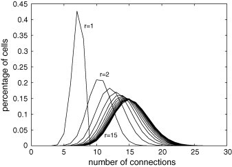
Degree distribution for and . The vertical axis indicates the percentage of the 40,000 () cells presenting the number of connections shown in the horizontal axis. For instance, for , then about 20% of cells have 10 connections. By increasing the value of r, the distribution peak decreases, and the distribution width and the average value increase.
Fig. 2.
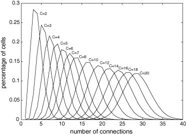
Degree distribution for and . By increasing the value of C, the distribution peak decreases, and the distribution width and the average value increase.
The clustering coefficient is the typical number of connections existing between cells pertaining to a neighborhood of a cell divided by the total number of connections that could possibly exist. The higher this coefficient, the quicker the disease can spread into the neighborhood. Fig. 3 shows that this coefficient increases with C and tends to decrease with r.
Fig. 3.
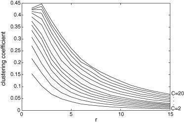
Clustering coefficient for and . The value of r appears in the horizontal axis and the value of C in the right edge. This topological parameter tends to decrease with r and it increases with C.
The average shortest path length is the average shortest distance between any two cells composing the lattice. If this path length is small, then two cells are usually connected by just a few connections, which facilitates the disease propagation. Fig. 4 evidences that this length decreases with increasing values of r and/or C.
Fig. 4.
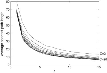
Average shortest path length for and . The value of r is given in the horizontal axis and the value of C in the right edge. This topological parameter decreases with r and/or C.
The influence of these topological parameters in the disease propagation are investigated in Section 4. In the next section, the epidemiological models based on PCA and ODE are presented.
3. PCA and ODE approaches
Each cell in the PCA lattice represents an individual that can be in one of three states: S, I or R. The time evolution of this population is ruled by the following set of probabilities of state transitions. At each time step, there is a probability of a S-cell being infected according to , where is the number of connections with infective neighbors and k is a parameter related to the disease infectivity (observe that is a monotone increasing function of , and that , but ). Each I-cell has probability per time step of becoming cured and probability per time step of dying because of the disease. At each iteration, recovered cells may die due to other causes with probability . When infective and recovered individuals die, susceptible ones replace them. Therefore, the total number of individuals remains constant; an appropriate assumption for modelling diseases spreading quickly and/or populations where the deaths are balanced by the births. The states of all cells are simultaneously updated throughout a simulation.
This PCA model is a variation of the model proposed by Monteiro et al. (2006a). There an I-cell could also die by other causes and the neighborhood of a cell was restricted to its eight surrounding cells. Here an I-cell can die only because of the disease and the connections with other cells are determined by applying Eq. (1) at each time step. Thus, the neighbors may not be local and may not be the same from one time step to another.
If S, I and R-individuals are homogeneously distributed over the space, then this PCA can be represented by the following ODE model:
| (2) |
where a is the infection rate constant; b is the recovering rate constant; c is the death rate constant related to the disease; e is the death rate constant related to other causes. Because , the total number of individuals remains constant, thus: .
The stationary solutions (where , and are constants satisfying , , for any instant t) of Eq. (2) are
| (3) |
and
| (4) |
where
| (5) |
Stability analysis of Eq. (2) Monteiro et al., 2006a, Monteiro et al., 2007 reveals that the disease-free stationary state given by Eq. (3) is asymptotically stable if and unstable if ; the endemic stationary state given by Eq. (4) is unstable if and asymptotically stable if . For this ODE model, the bifurcation parameter defined by Eq. (5) corresponds to the basic reproduction number. In fact, each different epidemiological model yields a different expression to (e.g. Piqueira et al., 2004).
Because the ODE model is a mean-field approximation for the PCA model, the values of the epidemiological parameters a, b, c and e can be estimated from PCA simulations by the following expressions obtained from Eq. (2):
| (6) |
where is the increase per time step of infective individuals due to the contamination process; is the increase per time step of recovered individuals due to the healing process; is the increase per time step of susceptible individuals due to the death caused by the disease; and is the increase per time step of susceptible individuals due to the death for other causes. By assuming that the probability of a state transition at each iteration can be estimated from the relative frequency of its occurrence, then ; ; ; . Therefore:
| (7) |
where is the number of susceptible cells with connections to infective neighbors. The expression for the parameter c is due to the fact that, at the time step t, an infective cell is firstly tested if it will be cured (with probability ) at ; if not cured, then it is tested if will be dead (with probability ) at .
Thus, the epidemiological parameters b, c and e appearing in the linear terms of Eq. (2) are related to the probabilities of recovering and dying. The value of a is related to the average infection probability and it is the unique epidemiological parameter influenced by r and C.
By using Eq. (6), simulations with the PCA model can be performed for estimating the values of the parameters a, b, c and e appearing in the ODE model, in order to obtain similar evolutions of , and in both approaches. Average values of these four epidemiological parameters are calculated by taking into account the last 20 time steps of a PCA simulation (when the system already reached its permanent regime). Then, these average values are substituted in Eq. (2), which are numerically solved.
Figs. 5(left) and 6(left) show the dynamical behaviors of the PCA for , , %, %, %; Figs. 5(right) and 6(right) exhibit the temporal evolutions of the corresponding ODE with the parameter values determined by Eq. (6). At , S, I and R-cells are randomly distributed according to the proportions %, %, %. In Fig. 5(left), for and the corresponding numerical value of the basic reproduction number obtained from Eqs. (5), (6) is ; in Fig. 6(left) for and , . Observe the good agreement between the two approaches.
Fig. 5.
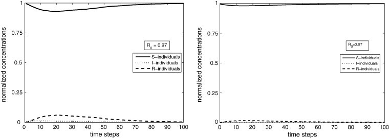
PCA (left) and ODE (right) simulations for and . As , the disease-free stationary state is reached in the permanent regime.
Fig. 6.
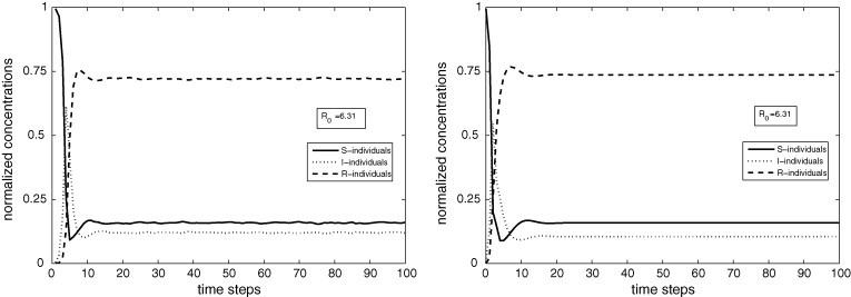
PCA (left) and ODE (right) simulations for and . As , the endemic stationary state is reached in the permanent regime.
Fig. 7 shows the asymptotically stable stationary solutions in function of . As predicted from the ODE analyses, the disease only persists in the PCA simulations if .
Fig. 7.
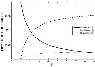
Asymptotically stable values of , and in function of obtained from Eqs. (3), (4) for the same epidemiological parameter values used in Fig. 5, Fig. 6 (i.e., , , ).
4. Influence of the contact network on the disease dynamics
The aim here is to understand how the values of r, C and the two topological parameters described in Section 2 affect , the permanent regime and the transient behavior of the PCA model. In this section, all figures show average results obtained in ten simulations with the same epidemiological parameter values used in Fig. 5, Fig. 6, Fig. 7. Thus, changes because r and/or C (and consequently a) vary. In each simulation, S, I and R-cells in the PCA lattice are randomly distributed at respecting the proportions used in Fig. 5, Fig. 6, Fig. 7. Hence, the numerical values of the initial conditions are the same, but the corresponding geographical distributions may be altered from one simulation to another. And, from a time step to another, the neighborhood of each cell is recreated by following Eq. (1). Other sets of epidemiological parameter values (for instance, , %, %, %) and/or initial conditions (for instance, %, %, %) were tested, and the results were qualitatively the same as reported below.
Fig. 8 presents in function of r and C for and (the disease frequently disappears for and any r, and and ; for the other values of C and r it usually persists). Notice that increases with r and/or C (because a increases with r and/or C) and reaches a limit. Thus, the increase of the number of contacts (obtained from the parameter C) and the increase of the area where these contacts are made (related to the parameter r) help to support the persistence of a disease in a population.
Fig. 8.
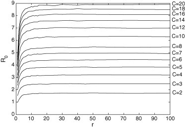
for and . The higher the value of r and/or C, the higher .
Fig. 9, Fig. 10, Fig. 11 illustrate the asymptotically stable stationary concentrations of S, I and R in function of r and C for and . The values of and grow with increases in r and/or C; the value of diminishes. Observe that all these stationary concentrations attain limit values when the interactions among individuals are amplified. Observe also that densely connected populations present higher infective and recovered individuals than sparsely coupled populations.
Fig. 9.
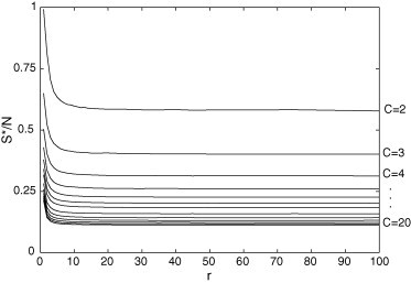
for and . In the permanent regime, the susceptible group decreases with r and/or C.
Fig. 10.
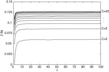
for and . In the permanent regime, the infective group increases with r and/or C.
Fig. 11.
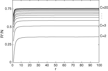
for and . In the permanent regime, the recovered group increases with r and/or C.
Fig. 12, Fig. 13, Fig. 14 are related to some features of the transient behavior of in the PCA model. These features are: the maximum peak, the instant when this peak occurs, and the settling time (here defined as the first time instant T where the average value of in does not vary more than 3% of its stationary value). Fig. 12 shows that the maximum peak increases with r and it increases with C until ; from to , this peak decreases as C grows. This is an interesting result because a lower maximum peak cannot be due to a less infectious disease or a more resistant population; it can be caused by increasing the number of connections beyond a critical value. Fig. 13, Fig. 14 reveal that, after an initial growing, the peak instant and the settling time tend to decrease as r grows. The values of both these transitory features diminish when C increases.
Fig. 12.

Maximum peak of in the PCA model for and (left) (right). The highest concentration of initially increases with r and then reaches a saturation value, and there is a value of C for which this transient feature attains its maximum.
Fig. 13.
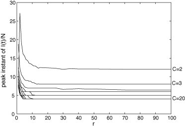
Peak instant of in the PCA model for and . The instant corresponding to the highest concentration of decreases with C, and there is a value of r (usually a low value) for which this transient feature reaches its maximum.
Fig. 14.
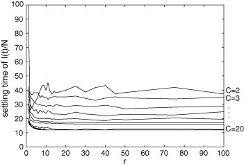
Settling time of in the PCA model for and . The interval time needed for the system reaching its permanent regime tends to decrease with C, and there is a value of r (usually a low value) for which this transient feature attains its maximum.
The relation between maximum peak of and is far from being trivial, as shown in Fig. 15 ; however, there is a tendency of increasing. Fig. 16, Fig. 17 reveal that the peak instant and the settling time of depend on in a similar way that they depend on r (Fig. 13, Fig. 14). Thus, these both features initially increase with and then, after a critical number, they decrease and saturate. Fig. 16, Fig. 17 show that (for the epidemiological parameter values used in these simulations) a disease with and another with can present similar peak instants and similar settling times; therefore, these transitory features alone cannot be adequate for distinguishing them in terms of .
Fig. 15.
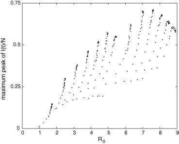
Maximum peak of in the PCA model in terms of . Notice that a particular value of this transient feature can correspond to different values of .
Fig. 16.
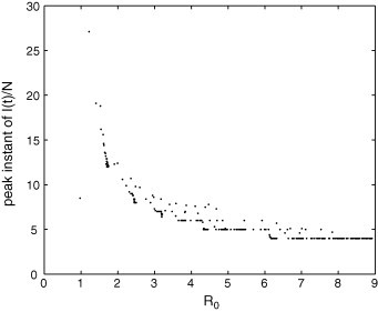
Peak instant of in the PCA model in terms of . Observe that a particular value of this transient feature can correspond to distinct values of .
Fig. 17.
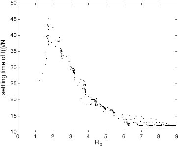
Settling time of in the PCA model in terms of . Notice that a particular value of this transient feature can correspond to unalike values of .
Fig. 8 shows that the number increases with r and/or C (according to Eq. (5) is proportional to the epidemiological parameter a, which increases with r and/or C). Because the clustering coefficient and the average shortest path length vary with r and C as exhibited by Fig. 3, Fig. 4, it is interesting to understand how these two topological parameters are related to .
The relation between clustering coefficient and is illustrated in Fig. 18 . For a fixed value of C, this coefficient decreases with because higher values of are due to higher values of r. Thus, by increasing the area where the contacts are made and keeping fixed the number of connections, the clustering coefficient must diminish, because connections between cells composing the neighborhood of a particular cell become more rare. The higher this fixed value of C, the higher the value of this coefficient. For a fixed value of r, the clustering coefficient increases with because higher values of are due to higher values of C. Therefore, by increasing the number of connections and keeping fixed the area where they are made, the clustering coefficient must increase, because more links between cells composing the neighborhood of a particular cell can be established. The higher this fixed value of r, the smaller the value of this coefficient.
Fig. 18.
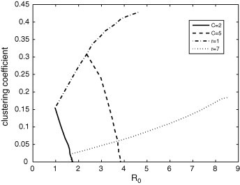
Clustering coefficient in function of for some fixed values of r and C. By keeping C constant, this coefficient decreases with because higher values of correspond to higher values of r. By keeping r constant, this coefficient increases with because higher values of correspond to higher values of C.
Fig. 19 reveals that the average shortest path length decreases with the value of , either by increasing the number of connections or the neighborhood area. Higher values of r and/or C imply smaller path lengths between two cells.
Fig. 19.
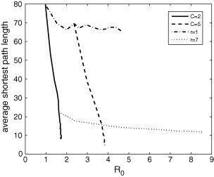
Average shortest path length in function of for some fixed values of r and C. By keeping C constant, this length decreases with because higher values of correspond to higher values of r. By keeping r constant, this length also tends to decrease with because higher values of correspond to higher values of C.
Fig. 18, Fig. 19 show that a same value of is compatible with distinct values of clustering coefficient (cc) and average shortest path length (l) for a given disease. For instance, a disease characterized by is compatible with a network with and and with another network with and .
5. Discussion
The random coupling topology described by Eq. (1) is function of the parameters r (related to the area where connections between cells can be made) and C (expressing the number of connections starting from each cell). Fig. 8 shows that , a bifurcation parameter in the dynamical system jargon, increases with r and/or C. When this parameter is above a critical value (1, by definition), then the model used for deriving the analytical expression for predicts that the disease will spread in the population. There are reports about severe epidemics occurred in slave ships during the 19th century (e.g. Watts, 1999). This is a historic example illustrating the influence of C on disease spreadings. Slaves had a very limited value of r, but the increase of C caused by gathering them in a ship increased the value of of such a population, which made easier the propagation of diseases. Cases illustrating the influence of r in disease propagations can also be easily found. For instance, sailing ships developed mainly from the 13th century amplified the human mobility on the world; consequently, the value of r and the incidence of epidemics. A classical example is the devastation of the Aztec population by smallpox in the 16th century after the Spanish invasion (e.g. Watts, 1999).
Beyond the predictive power of (questioned by some authors, e.g. Alves et al., 2003, Cross et al., 2007), its numerical value is important because it gives hints of the effort required to contain a disease spreading. For instance, Bauch and Earn (2004) proposed a game theoretical framework to analyze, in function of , how the morbidity risk perception associated to voluntary vaccination policies influence the course of epidemics. Shulgin et al. (1998) used a SIR model based in ODE to determine, in terms of , the minimum percentage p of susceptible individuals that must be vaccinated to eradicate a contagious disease; they found . This expression was also derived by Huang (2008) from a SEIR model (where E represents the exposed (latent) group), who applied it for calculating the critical vaccination level associated to 21 well-known infectious diseases. A similar expression was obtained by Farrington (2003) considering the vaccine efficacy.
The value of can be unambiguously determined from the asymptotical stable stationary concentrations (as shown in Fig. 7); however, public health departments cannot wait for the SIR system reaching its permanent regime to specify the control strategies. Thus, there are attempts of estimating the value of from the transient features of (e.g., Roberts and Heesterbeek, 2007). For instance, the classical SIR model can be obtained from Eq. (2) by imposing and . In this model based on differential equations by supposing that the groups of S, I and R are homogeneously mixed, and the maximum peak of , , is given by (e.g. Murray, 2003):
| (8) |
Thus, in this model is directly related to the normalized value of the maximum peak (assuming that , i.e., almost all population is initially susceptible). By using a model taking into account the spatial relations among the individuals, here we found that the maximum peak of , the corresponding peak instant and the settling time may not be appropriate for estimating .
We also showed that a same value of can be associated to networks with distinct values of clustering coefficient and average shortest path length. This result can affect the evaluation of the effectiveness concerning different strategies employed for controlling a disease spreading. For instance, Lipsitch et al. (2003) and Zhang (2007) studied the transmission dynamics of the severe acute respiratory syndrome (SARS) by using mathematical models that do not explicitly consider the geographical localizations of the individuals, and they concluded that in the absence of control measures. Because distinct values of topological properties can produce the same value of in a model considerating the spatial structure of the contact network, it is difficult to evaluate the effective contribution of each control measure, like isolations of SARS cases, quarantine of their asymptomatic contacts and restrictions on long-range population movement. Of course, all these interventions decrease (r and C, and consequently) and help to reduce the transmission. However, the weight of each intervention in the global result is far from being understood, possibly because the correspondences among and the topological properties of the contact network are not one-to-one. Another example: Chen et al. (2006) quantified the impact of distinct control measures (such as filtration, isolation, vaccination) in containing the propagation of indoor airborne infections (like chickenpox, influenza, measles, SARS); however, they did not take into account the contact network. These authors proposed to explicitly consider this network in their model, in order to get more accurate predictions. Based in our results, we do agree with them.
Let a contagious disease and a host population be characterized by the epidemiological and topological parameters k, b, c, e, r and C (according to our SIR models). Future works should try to answer the following questions:
-
(1)
Can this disease be eradicated by isolating a fraction F of I-individuals? Or, is there a critical value so that if the fraction of the I-individuals is isolated, then the disease is eradicated? In other words, is this unique procedure enough to reduce the effective value of (that is, the value of for a disease propagating in a population employing control measures) below 1? Observe that isolation means strong reduction in the values of r and C for I-individuals and, consequently, alteration in the topological properties of the contact network.
-
(2)
Preventive attitudes (as the use of masks against airborne infections or condoms against sexually transmitted diseases) alter the coupling topology of the S-individuals. Can this disease be eradicated if a fraction F of S-individuals have preventive attitudes? Is there a critical value so that if the fraction of the S-individuals takes precaution measures, then the disease is eradicated? In other words, the effective value of can be decreased below 1 only with these attitudes?
-
(3)
Our simulations showed that random contact networks with distinct topological parameter values can result in the same value of for the same disease. One can wonder if the two control strategies mentioned in the items (1) and (2) when separately applied against a particular disease would lead to networks with distinct topological features but with similar values of .
-
(4)
Which of these two strategies can reduce below 1 requiring the lowest value of ?
-
(5)
Vaccination is frequently modelled either as a conversion of S-individuals to R-individuals or as a decreasing in the birth rate of S-individuals (e.g. Bauch and Earn, 2004, Shulgin et al., 1998). Thus, this control strategy seems not be directly related to changes in the topological properties of the contact network. However, if there exists a vaccine against the disease under analysis, what is the optimum combination among these strategies (isolation, prevention, vaccination) in order to eradicate such a disease? Here “optimum” can be interpreted as lowest cost and/or highest quality of life.
Acknowledgement
LHAM is partially supported by CNPq.
Contributor Information
P.H.T. Schimit, Email: pedro.schimit@poli.usp.br.
L.H.A. Monteiro, Email: luizm@mackenzie.br, luizm@usp.br.
References
- Ahmed E., Agiza H.N., Hassan S.Z. On modeling Hepatitis B transmission using cellular automata. J. Stat. Phys. 1998;92:707–712. [Google Scholar]
- Alves D., Haas V.J., Caliri A. The predictive power of in an epidemic probabilistic system. J. Biol. Phys. 2003;29:63–75. doi: 10.1023/A:1022567418081. [DOI] [PMC free article] [PubMed] [Google Scholar]
- Anderson R.M., May R.M. Oxford University Press; Oxford: 1992. Infectious Diseases of Humans: Dynamics and Control. [Google Scholar]
- Barabasi A.L. Plume; London: 2003. Linked: How Everything Is Connected to Everything Else and What It Means. [Google Scholar]
- Bauch C.T., Earn D.J.D. Vaccination and the theory of games. Proc. Natl. Acad. Sci. U.S.A. 2004;101:13391–13394. doi: 10.1073/pnas.0403823101. [DOI] [PMC free article] [PubMed] [Google Scholar]
- Bollobàs B. Cambridge University Press; Cambridge: 2001. Random Graphs. [Google Scholar]
- Boccaletti S., Latora V., Moreno Y., Chavez M., Hwang D.U. Complex networks: structure and dynamics. Phys. Rep. 2006;424:175–308. [Google Scholar]
- Chen S.C., Chang C.F., Liao C.M. Predictive models of controls strategies involved in containing indoor airborne infections. Indoor Air. 2006;16:469–481. doi: 10.1111/j.1600-0668.2006.00443.x. [DOI] [PubMed] [Google Scholar]
- Cross P.C., Johnson P.L.F., Lloyd-Smith J.O., Getz W.M. Utility of as a predictor of disease invasion in structured populations. J. R. Soc. Interface. 2007;4:315–324. doi: 10.1098/rsif.2006.0185. [DOI] [PMC free article] [PubMed] [Google Scholar]
- Doran J.R., Laffan S.W. Simulating the spatial dynamics of foot and mouth disease outbreaks in feral pigs and livestock in Queensland, Australia, using a susceptible-infected-recovered cellular automata model. Prev. Vet. Med. 2005;70:133–152. doi: 10.1016/j.prevetmed.2005.03.002. [DOI] [PubMed] [Google Scholar]
- Farrington C.P. On vaccine efficacy and reproduction numbers. Math. Biosci. 2003;185:89–109. doi: 10.1016/s0025-5564(03)00061-0. [DOI] [PubMed] [Google Scholar]
- Fuentes M.A., Kuperman M.N. Cellular automata and epidemiological models with spatial dependence. Physica A. 1999;267:471–486. [Google Scholar]
- Hartvigsen G., Dresch J.M., Zielinski A.L., Macula A.J., Leary C.C. Network structure, and vaccination strategy and effort interact to affect the dynamics of influenza epidemics. J. Theor. Biol. 2007;246:205–213. doi: 10.1016/j.jtbi.2006.12.027. [DOI] [PubMed] [Google Scholar]
- Huang S.Z. A new SEIR epidemic model with applications to the theory of eradication and control of diseases, and to the calculation of . Math. Biosci. 2008;215:84–104. doi: 10.1016/j.mbs.2008.06.005. [DOI] [PubMed] [Google Scholar]
- Kansal A.R., Torquato S., Harsh G.R., Chiocca E.A., Deisboeck T.S., IV Simulated brain tumor growth dynamics using a three-dimensional cellular automaton. J. Theor. Biol. 2000;203:367–382. doi: 10.1006/jtbi.2000.2000. [DOI] [PubMed] [Google Scholar]
- Kleczkowski A., Grenfell B.T. Mean-field-type equations for spread of epidemics: the “small world” model. Physica A. 1999;274:355–360. [Google Scholar]
- Lipsitch M., Cohen T., Cooper B., Robins J.M., Ma S., James L., Gopalakrishna G., Chew S.K., Tan C.C., Samore M.H., Fisman D., Murray M. Transmission dynamics and control of severe acute respiratory syndrome. Science. 2003;300:1966–1970. doi: 10.1126/science.1086616. [DOI] [PMC free article] [PubMed] [Google Scholar]
- Monteiro L.H.A., Chimara H.D.B., Berlinck J.G.C. Big cities: shelters for contagious diseases. Ecol. Model. 2006;197:258–262. [Google Scholar]
- Monteiro L.H.A., Paiva D.C., Piqueira J.R.C. Spreading depression in mainly locally connected cellular automaton. J. Biol. Syst. 2006;14:629–671. [Google Scholar]
- Monteiro L.H.A., Sasso J.B., Berlinck J.G.C. Continuous and discrete approaches to the epidemiology of viral spreading taking into account the delay of incubation time. Ecol. Model. 2007;201:553–557. [Google Scholar]
- Murray J.D. Springer; New York: 2003. Mathematical Biology I: An Introduction. [Google Scholar]
- Newmann M.E.J. Spread of epidemic disease on networks. Phys. Rev. E. 2002;66:016128. doi: 10.1103/PhysRevE.66.016128. [DOI] [PubMed] [Google Scholar]
- Nishiura H., Inaba H. Discussion: emergence of the concept of the basic reproduction number from mathematical demography. J. Theor. Biol. 2007;244:357–364. doi: 10.1016/j.jtbi.2006.08.004. [DOI] [PubMed] [Google Scholar]
- Pautasso M., Jeger M.J. Epidemic threshold and network structure: the interplay of probability of transmission and of persistence in small-size directed networks. Ecol. Compl. 2008;5:1–8. [Google Scholar]
- Piqueira J.R.C., Castaño M.C., Monteiro L.H.A. Modeling the spreading of HIV in homosexual populations with heterogeneous preventive attitude. J. Biol. Syst. 2004;12:439–456. [Google Scholar]
- Roberts M.G., Heesterbeek J.A.P. Model-consistent estimation of the basic reproduction number from the incidence of an emerging infection. J. Math. Biol. 2007;55:803–816. doi: 10.1007/s00285-007-0112-8. [DOI] [PMC free article] [PubMed] [Google Scholar]
- Shulgin B., Stone L., Agur Z. Pulse vaccination strategy in the SIR epidemic model. Bull. Math. Biol. 1998;60:1123–1148. doi: 10.1006/S0092-8240(98)90005-2. [DOI] [PubMed] [Google Scholar]
- Sirakoulis G.Ch., Karafyllidis I., Thanailakis A. A cellular automaton model for the effects of population movement and vaccination on epidemic propagation. Ecol. Model. 2000;133:209–223. [Google Scholar]
- Ward M.P., Laffan S.W., Highfield L.D. The potential role of wild and feral animals as reservoirs of foot-and-mouth disease. Prev. Vet. Med. 2007;80:9–23. doi: 10.1016/j.prevetmed.2007.01.009. [DOI] [PubMed] [Google Scholar]
- Watts S. Yale University Press; Yale: 1999. Epidemics and History: Disease, Power and Imperialism. [Google Scholar]
- Watts D.J., Strogatz S.H. Collective dynamics of small-world networks. Nature. 1998;393:440–442. doi: 10.1038/30918. [DOI] [PubMed] [Google Scholar]
- Wolfram S. Westview Press; New York: 1994. Cellular Automata and Complexity: Collected Papers. [Google Scholar]
- Xu X.J., Wang W.X., Zhou T., Chen G. Geographical effects on epidemic spreading in scale-free networks. Int. J. Mod. Phys. C. 2006;17:1815–1822. [Google Scholar]
- Yakowitz S., Gani J., Hayes R. Cellular automaton modeling of epidemics. Appl. Math. Comput. 1990;40:41–54. [Google Scholar]
- Zhang Z. The outbreak pattern of SARS cases in China as revealed by mathematical model. Ecol. Model. 2007;204:420–426. doi: 10.1016/j.ecolmodel.2007.01.020. [DOI] [PMC free article] [PubMed] [Google Scholar]


