Identifying Spatial Invasion of Pandemics on Metapopulation Networks Via Anatomizing Arrival History

Abstract

Spatial spread of infectious diseases among populations via the mobility of humans is highly stochastic and heterogeneous. Accurate forecast/mining of the spread process is often hard to be achieved by using statistical or mechanical models. Here we propose a new reverse problem, which aims to identify the stochastically spatial spread process itself from observable information regarding the arrival history of infectious cases in each subpopulation. We solved the problem by developing an efficient optimization algorithm based on dynamical programming, which comprises three procedures: 1) anatomizing the whole spread process among all subpopulations into disjoint componential patches; 2) inferring the most probable invasion pathways underlying each patch via maximum likelihood estimation; and 3) recovering the whole process by assembling the invasion pathways in each patch iteratively, without burdens in parameter calibrations and computer simulations. Based on the entropy theory, we introduced an identifiability measure to assess the difficulty level that an invasion pathway can be identified. Results on both artificial and empirical metapopulation networks show the robust performance in identifying actual invasion pathways driving pandemic spread.

I. Introduction

The frequent outbreaks of emerging infectious diseases in recent decades lead to great social, economic, and public health burdens [1]–[3]. This trend is partially due to the urbanization process and, in particular, the establishment of long-distance traffic networks, which facilitate the dissemination of pathogens accompanied with passengers [4], [5]. Real-world examples include the transnational spread of severe acute respiratory syndrome (SARS)-coronavirus in 2003 [6], the global outbreak of A (H1N1) pandemic flu in 2009 [7], [8], avian influenza in Southeast Asia [9], [10], the spark of Ebola infections in western countries in 2014 [11], and recent potential outbreak of middle east respiratory syndrome [12].

During almost the same epoch, the theory of complex networks has been developed as a valuable tool for modeling the structure and dynamics of/on complex systems [13]–[16]. In the study of network epidemiology, networks are often used to describe the epidemic spreading from human to human via contacts, where nodes represent persons and edges represent interpersonal contacts [17]–[22]. To characterize the spatial spread between different geo-locations, simple network models are generalized with metapopulation framework, in which each node represents a population of individuals that reside at the same geo-region (e.g., a city), and the edge describes the traffic route that drives the individual mobility between populations [18], [19]. The networked metapopulation models have been applied to study the real-world cases such as SARS [6], A (H1N1) pandemic flu [23], and Ebola [11], which can capture some key dynamic features including peak times, basic epidemic curves, and epidemic sizes. Quantitative model results can be used to evaluate the effectiveness of control strategies [24]–[28], such as optimizing the vaccine allocation.

The numerical computing of large-scale metapopulation models is time-consuming, because of the requirement of high-level computer power. The model calibrations need high-resolution data for incidence cases, which may not be available or accurate during the early weeks of initial outbreaks [4]. Hence, continuous model training with data collected in real-time is essential in achieving a reliable model prediction [29]. Generally, model results are the ensemble average over numerous simulation realizations, which aims to predict the mean and variance of epidemic curves, while in reality there is no such thing described by the average over different realizations [30]. To extract more meaningful information from epidemic data generated by surveillance systems, recent studies (particularly in engineering fields) start paying attention to reverse problems, such as source detection and network reconstruction, which are briefly summarized here.

A. Related Works

The theory of system identification has been established in engineering fields, usually used to infer system parameters. The use of system identification in epidemiology mainly focuses on inferring epidemic parameters, such as the transmission rate and generation time [31], which relies on constructing dynamical systems of ordinary differential equations. The methodology of system identification is not helpful in solving high-dimensional stochastic many-body systems, such as metapopulation models.

Source detection for rumor spreading on complex networks is becoming a popular topic, attracting extensive discussions in recent years. The target is to figure out the causality that can trigger the explosive dissemination across social networks, such as Facebook, Twitter, and Weibo. For example, using maximum likelihood (ML) estimators, Shah and Zaman [32] proposed the concept of rumor centrality that quantifies the role of nodes in network spreading. Luo et al. [33] designed new estimators to infer infection sources and regions in large networks. Wang et al. [34], [36] and Dong et al. [35] extended the scope by using multiple observations, which largely improves the detection accuracy. Another interesting topic is the network inference, which engages in revealing the topology structure of a network from the hint underlying the dynamics on a network [37]. Some useful algorithms (e.g., NetInf) have been proposed in [38]–[42]. Note that the algorithms for source detection and network inference are not feasible in identifying the spreading processes on metapopulation networks.

Using metapopulation networks models, some heuristic measures have been proposed to understand the spatial spread of infectious diseases, which are most related to this paper. Gautreau et al. [30] developed an approximation for the mean first arrival time between populations that have direct connection, which can be used to construct the shortest path tree (SPT) that characterizes the average transmission pathways among populations. Brockmann and Helbing [4] proposed a measure called “effective distance,” which can also be used to build the SPT. Using a different method based on the ML, Balcan et al. [43] generated the transmission pathways by extracting the minimum spanning tree from extensive Monte Carlo simulation results. Details about these measures will be given in Section IV, which compares the algorithmic performance.

B. Motivation

Current algorithms to inferring pandemic spatial spread generally make use of the topology features of metapopulation networks or extensive epidemic simulations. The resulting outcome is an ensemble average over all possible transmission pathways, which may fail in capturing those indeed transmitting the disease between populations, because of the high-level stochasticity and heterogeneity in the spreading process.

Good news comes from the development of modern sentinel and Internet-based surveillance systems, which becomes increasingly popular in guiding public health control strategies. Such systems can or will provide high-resolution, location-specific data on human and poultry cases [44]. Human mobility data are also available from mass transportation systems or GPS-based mobile Apps [3]. Integrating these data often used in different fields, a natural reverse problem poses itself, which is the central interest of this paper: is it probable to design an efficient algorithm to identify or retrospect the stochastic pandemic spatial spread process among populations by linking epidemic data and models.

C. Our Contributions

Main contributions of this paper are as follows.

• 1)A novel reverse problem of identifying the stochastic pandemic spatial spread process on metapopulation networks is proposed, which cannot be solved by existing techniques.
• 2)An efficient algorithm based on dynamical programming is proposed to solve the problem, which comprises three procedures. First, the whole spread process among all populations will be decomposed into disjoint componential patches, which can be categorized into four types of invasion cases (INCs). Then, since two types of INCs contain hidden pathways, an optimization approach based on the ML estimation is developed to infer the most probable invasion pathways underlying each path. Finally, the whole spread process will be recovered by assembling the invasion pathways of each patch chronologically, without burdens in parameter calibrations and computer simulations.
• 3)An entropy-based measure called identifiability is introduced to depict the difficulty level an INC can be identified. Comparisons on both artificial and empirical networks show that our algorithm outperforms the existing methods in accuracy and robustness.

The remaining sections are organized as follows. Section II provides the preliminary definitions and problem formulation. Section III describes the procedures of our identification algorithm, and introduces the identifiability measure. Section IV performs computer experiments to compare the performance of algorithms. Section V gives the conclusion.

II. Preliminary and Problem Formulation

This section first elucidates the structure of networked metapopulation model, and then provides the preliminary definitions and problem formulation.

A. Networked Metapopulation Model

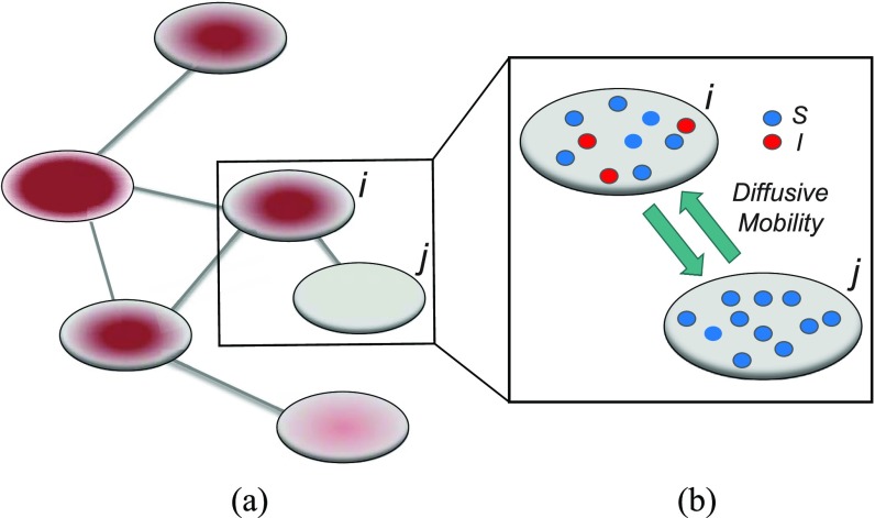
In the networked metapopulation model, individuals are organized into social units such as counties and cities, defined as subpopulations, which are interconnected by traffic networks of transportation routes. The disease prevails in each subpopulation due to interpersonal contacts, and spreads between subpopulations via the mobility of infected persons. Fig. 1 illustrates the model structure.

Fig. 1.

Illustration of a networked metapopulation model, which comprises six subpopulations/patches that are coupled by the mobility of individuals. In each subpopulation, each individual can be in one of two disease statuses (i.e., susceptible and infectious), shown in different colors. Each individual can travel between connected subpopulation. (a) Networked metapopulation. (b) Two subpopulations.

Within each subpopulation, individuals mix homogeneously. This assumption is partially supported by recent empirical findings on intraurban human mobility patterns [19], [45]–[48]. The intrapopulation epidemic dynamics are characterized by compartment models. Considering the wide applications in describing the spread of pathogens, species, rumors, emotion, behavior, crisis, etc. [32], [33], [35], [49], we used the susceptible-infected (SI) model in this paper. Define as the population size of each subpopulation , the number of infected cases in subpopulation at time , the transmission rate that an infected host infects a susceptible individual shared the same location in unit time. As such, the risk of infection within subpopulation at time is characterized by . Per unit time, the number of individuals newly infected in subpopulation can be calculated from a binomial distribution with probability and trails equalling the number of susceptible persons .

The mobility of individuals among subpopulations is conceptually described by diffusion dynamics, , where is a placeholder for or , is the set of subpopulations directly connected with subpopulation , and is the per capita mobility rate from subpopulation to , which equals the ratio between the daily flux of passengers from subpopulation to and the population size of departure subpopulation . The ensemble of mobility rates defines a transition matrix , determined by the topology structure and traffic fluxes of the mobility network. The interpopulation mobility of individuals is simulated with binomial or multinomial process (Appendix A). For more details in modeling rules, refer to [19].

B. Basic Definitions

The epidemic arrival time (EAT) is the first arrival time of infectious hosts traveling to a susceptible subpopulation. At a given EAT, at least an unaffected (susceptible) subpopulation will be contaminated, characterizing the occurrence of invasion events. Herein, S (I) denotes a (an) susceptible (infected) subpopulation.

For an invasion event, organizing newly contaminated subpopulations (remaining unaffected prior to that invasion event) into set , and infected subpopulations into set , we define the four types of INC as follows.

• 1): and both are composed of a single subpopulation respectively, which represents that a previously unaffected subpopulation is infected by the new arrival of infectious host(s) from its unique neighboring infected subpopulation.
• 2): In this case, only consists of a single subpopulation, while contains subpopulations. This represents that previously unaffected subpopulations are contaminated due to the new arrival of infectious hosts from their common infected subpopulation in .
• 3): only consists of a single subpopulation, and contains subpopulations. This means that the newly infected subpopulation in is infected by the arrival of infected host(s) from potential upstream subpopulations in through the invasion edges.
• 4): In this case, and both are composed of no less than two subpopulations, and they constitute a connected subgraph. Each previously unaffected subpopulation in is contaminated due to the simultaneous arrival of infected hosts from potential source subpopulations in . Each subpopulation in may lead to the contamination of at least one but no more than neighboring downstream subpopulations in through the invasion edges. Multiple edges between any pair of subpopulations are forbidden.

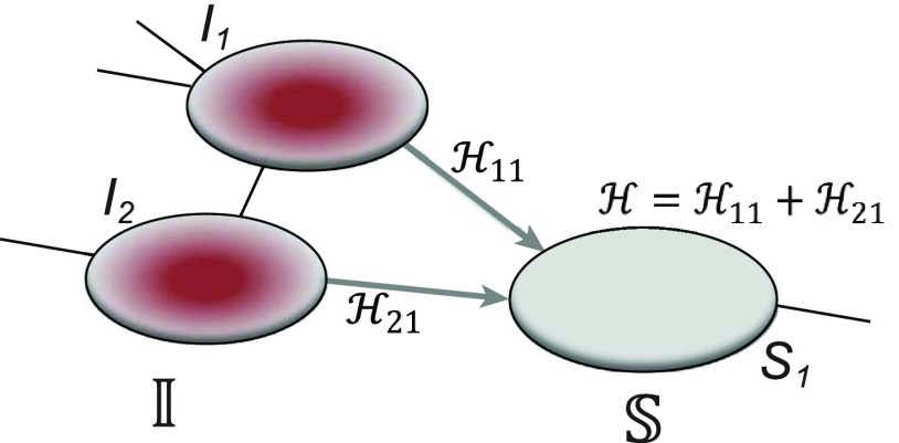
Fig. 2(a) and (b) illustrates the two scenarios of and . A decomposition procedure of invasion partition (INP) is used to generate the components of INCs in each invasion event. The heuristic search algorithm to proceed the INP is given in Algorithm 1 if an invasion event occurs.

Fig. 2.

(a) Example of the INC, in which infected subpopulations invade one susceptible subpopulation. The red patches denote the infected subpopulations, while the plain patch is the subpopulation that remains susceptible before time but will be contaminated during that time step due to the arrival of infectious cases from upstream infected subpopulations. (b) Example of the INC, in which infected subpopulations invade susceptible subpopulations.

Algorithm 1 INP

• 1:for an invasion event, collect all newly infected as initially and their previously infected neighbors as ;
• 2:start with an arbitrary element in set ;
• 3:find all neighbors of in set ;
• 4:find the new neighbors in the if have;
• 5:find the new neighbors in the if have;
• 6:repeat the above two steps until cannot find any new neighbors in and , we get an INC consisting of and , then update the and ;
• 7:repeat the 2-6 steps to get new INCs until there are no elements in .

C. Problem Formulation

Suppose that the spread starts at an infected subpopulation. It forms the invasion pathways when this source invades many susceptible subpopulations and the cascading invasion goes on. We record the infected individuals of each subpopulation per unit time. From the data, we should know when a subpopulation is infected and how many infected individuals in this subpopulation, but we may not know which infected subpopulations invade this subpopulation if it has (, ) infected neighbor subpopulations through the corresponding edge(s) [see Fig. 2(a)] at that time step. The question of interest is how to identify the instantaneous spatial invasion process just according to the surveillance data. Herein, we know the network topology including subpopulation size and travel flows, such as the city populations of airports and travelers by an airline of the real network of American airports network (ANN).

Define an invasion pathway which are the directed edges that infected individuals invade to susceptible subpopulations at EAT. To identify it, we proceed the following invasion pathways identification (IPI) algorithm.

• 1)
  Decompose the whole pathways as four types of INCs by the INP at each EAT; suppose the whole invasion pathways are anatomized into of four INCs. Let denote the identified invasion pathways based on the surveillance data of that INC and the given graph . According to the (stochastic) dynamic programming, we have the following equation to optimally solve this problem:

  
• 2)
  For each INC, we first judge whether it has a unique set of invasion pathways or more than one potential invasion pathways. When an INC has more than one possible invasion pathway, each set of which is called potential invasion pathway. If it has more than one potential invasion pathway, we estimate the true invasion pathways , denoted by , based on the surveillance data of that INC and the given graph . A potential pathway belonged to that INC is denoted by . To make this estimation, we shall compute the likelihood of a potential invasion pathway . With respect to this setting, the ML estimator of with respect to the networked metapopulation model given by that INC maximizes the correct identification probability. Therefore, we define the ML estimator

  

  where is the likelihood of observing the potential pathway assuming it is the true pathway . Thus we would like to evaluate for all and then choose the maximal one.

III. Identification Algorithm to Invasion Pathway

According to our above INP decompose algorithm, it is easy to identify the invasion pathways for the INC scenario (they have the only invasion pathway from their neighbor infected subpopulation). Thus our invasion pathways’ identification algorithm mainly deals with the other two kinds of INCs and . To make the description clear, we restate the term denotes subpopulation which is infected, and its number of infected individuals of at time is denoted by .

As time evolves, infected hosts travel among subpopulations, inducing the spatial pandemic dispersal. For each INC, by analyzing the variance of infected hosts in each subpopulation , we define three levels of extent of subpopulations observability to reflect the information held for the inference of relevant invasion pathway.

• 1)Observable Subpopulation: Subpopulation is observable during an INC, given the occurrence of the three most evident (subpopulation’s) status transitions. The first refers to the transition , accounting that the previously unaffected subpopulation is contaminated during that INC due to the arrival of infected hosts. The second concerns the transition , in which the previously infected subpopulation becomes susceptible again during that INC, since the infected hosts do not trigger a local outbreak and leave . In the third transition , despite of having infected subpopulations in the neighborhood, subpopulation remains unaffected during that INC due to no arrival of infected hosts. Fig. 3(a) illustrates such observable transitions.
• 2)Partially Observable Subpopulation: Subpopulation is partially observable during an INC occurring at time , if its number of infected hosts is decreased, i.e., and , which implies that at least infected hosts leave during that INC. It is impossible to distinguish their mobility destinations unless the INC or occurs. Fig. 3(b) illustrates the partially observable subpopulation.
• 3)Unobservable Subpopulation: Subpopulation is unobservable during an INC occurring at time , if its number of infected hosts has not been decreased, i.e., , considering the difficulty in judging whether there present infected hosts leaving subpopulation during that INC [see Fig. 3(c) for an illustration].

Fig. 3.

Illustration of neighbors classification in terms of status transitions: (a) Observable . (b) Partially observable . (c) Unobservable .

We further categorize the edges emanated from each infected subpopulation in set into four types, i.e., invasion edges, observable edges, partially observable edges, and unobservable edges.

• 1)Invasion Edges: In an INC, invasion edges represent each route emanated from subpopulation in to subpopulation in . They are considered as a unique category, because invasion edges contain all invasion pathway (an invasion pathway must be an invasion edge, but an invasion edge may not an invasion pathway). In Fig. 2(a) and (b), the invasion edges are illustrated. The following three types of edges are not belong to the routes between sets and , but they are the edges emanated from to subpopulation that is not belong to .
• 2)Observable Edges: For infected subpopulation in , any edge emanated from is observable, if it connects with observable subpopulation that only experiences the transition or from to . Here, it is intuitive that in subpopulation there is no arrival of infected hosts from subpopulation .
• 3)Partially Observable Edges: For infected subpopulation in , any edge is partially observable, if it connects with a partially observable subpopulation.
• 4)Unobservable Edges: For infected subpopulation in , any edge is unobservable, if it connects with an unobservable subpopulation.

The classification of subpopulations and edges are used to compute the corresponding subpopulation’s transferring estimator in Section III of both INCs of and .

A. Case of

As shown in Fig. 2(a), a typical INC is composed of two sets of subpopulations, i.e., the previously infected subpopulations and the previously unaffected subpopulation . Suppose that subpopulation is contaminated at time due to the appearance of infected hosts ( is a positive integer number) that come from the potential sources in . If the actual number of infected hosts from subpopulation is , , we have

with the conditions and .

1). Accurate Identification of Invasion Pathway:

Given a few satisfied prerequisites, (3) can has a unique solution, which implies that the invasion pathways of that INC can be identified accurately. Theorem 1 elucidates this scenario.

Theorem 1 (Accurate Identification of Invasion Pathway):

With the following conditions: 1) among possible sources illustrated in set , there are only partially observable subpopulations , whose neighboring subpopulations (excluding the invasion destination ) only experience the transition to or to at that EAT and 2) , the invasion pathway of an INC can be identified accurately.

Proof:

According to the definition of observability, in an INC, the number of local infected hosts in an involved partially observable source will be decreased by [ ] due to their departure. If the subpopulations in the neighborhood of only experience the transition of to or to from to , they are impossible to receive the infected hosts from subpopulation . Therefore, the newly contaminated subpopulation is the only destination for those infected travelers departing from the partially observable sources. Since , the second condition guarantees that (3) only has a unique solution, which corresponds to the accurate identification of invasion pathways of this INC.

2). Potential Invasion Pathway:

If the conditions of Theorem 1 are unsatisfied, (3) has multiple solutions, each solution corresponds to a set of potential invasion pathways that can result in the related INC. Due to the heterogeneity in the traffic flow on each edge and the number of infected hosts within each contaminated source, each set of potential pathways is associated with a unique likelihood, which also identifies the occurrence probability of the corresponding solution of (3). Therefore, the identification of invasion pathway that induce an INC can be transformed to searching the most probable solution of (3).

We define the solution space of (3) of the INC , which subjects to two conditions: 1) and 2) , . The second condition is obvious, since the number of infected travelers departing from the source cannot exceed . Let us assume that contains solutions, and a typical solution is formulated as . Obviously, each solution corresponds to a potential invasion pathway .

Through the INC , the observed event shows that the destination is contaminated due to the arrival of totally infected hosts from the potential sources . With this posterior information, we first measure the likelihood of each possible solution , which corresponds to the reasoning event that for each source , , infected hosts are transferred to . It is evident that , since will lead to the occurrence of event , which corresponds to .

According to Bayes’ theorem, the likelihood of the solution is characterized by

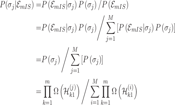where represents the number of potential solution , and the last item represents the mobility likelihood transferring estimator of infected subpopulation in .

One linchpin of our algorithm in handling the scenario is to estimate the probability of transferring infected hosts from each infected subpopulation to the destination subpopulation . Based on the independence between the intrasubpopulation epidemic reactions and the intersubpopulation personal diffusion, we introduce a transferring estimator to analyze the individual mobility of each source , which is in particular useful if there are partially observable and unobservable edges emanated from the focal infected subpopulation.

The specific formalisms of the transferring estimator are defined according to the three types of infected subpopulation consisted of set which are unobservable subpopulation, partially observable subpopulation, and observable subpopulation with transition of to .

a). Unobservable subpopulation :

Due to the occurrence of , among all edges emanated from subpopulation , there is only one invasion edge in that INC, labeled as , along which the traveling rate is and infected hosts are transferred to the destination . Assume that there are () unobservable and partially observable edges, labeled as , respectively. Along each unobservable or partially observable edge, the traveling rate is , , and infected hosts leave . Accordingly, in total infected hosts leave through the unobservable and partially observable edges. There remain observable edges, labeled as , respectively. Along each observable edge, the traveling rate is , , and infected hosts leave . With probability , an infected host keeps staying at source .

Since the infected hosts transferred by unobservable and partially observable edges are untraceable, it is unable to reveal the actual invasion pathways resulting in that INC accurately. Fortunately, the message of traveling rates on each edge is available by collecting and analyzing the human mobility transportation networks. Therefore, the mobility multinomial distribution [(31) in Appendix A] can be used to obtain the conditional probability that infected hosts are transferred from infected source to destination , which is measured by the following transferring estimator:

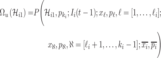where accounts for the number of infected hosts that do not leave source after the INC. Here, the observed number of infected persons in source before the INC, i.e., , is used for the estimation, since the probability that a newly infected host also experiencing the mobility process is very low. Considering the conservation of infected hosts, and the implication of observable edges (i.e., ), we have . Taking into account all scenarios that fulfill the condition , the transferring estimator is simplified by the marginal distribution of (4), that is

With independence, the transferring estimator becomes

b). Observable subpopulation ( to ):

If the infected hosts of source all leave to travel from to , the subpopulation is observable at that INC. In this case, we have additional posterior messages, i.e., and . Here, the number of infected hosts transferred to cannot exceed the total number of infected travelers departing from source , i.e., . In this regard, the probability that infected hosts arrive in destination is measured by the following transferring estimator:

c). Partially observable subpopulation :

If source is partially observable, we can develop the inference algorithm with an additional posterior message, which reveals that at least infected hosts leave the focal source after the occurrence of that INC. In order to measure the conditional probability that infected hosts are transferred from source to destination , we inspect all possible scenarios in detail, as follows.

Type 1: , i.e., the observed reduction in the number of infected hosts is less than those transferred from to . Here, we consider all cases that are in accordance with this condition.

If all confirmed infected travelers are transferred from to , the transferring estimator can be used to quantify the conditional probability that the remaining infected hosts concerned also visit , that is

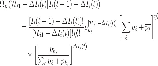where represents the relative traveling rate that any person from source is transferred to , thus the last item on the right-hand side (RHS) accounts for the probability that confirmed infected travelers all visit .

If only a fraction of confirmed infected travelers are transferred from to , the situation is more complicated. Assume that () confirmed travelers successfully come to , the corresponding transferring estimator becomes

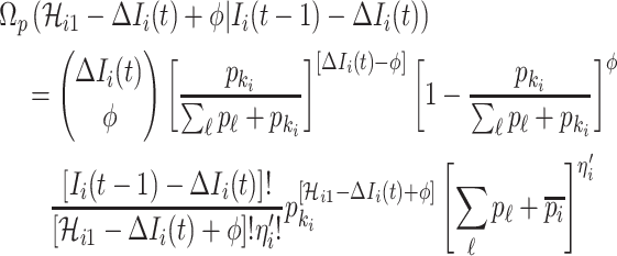where the first item on the RHS accounts for the probability that confirmed visitors visit .

If all confirmed infected travelers from are not transferred to , the conditional probability that among the remaining infected hosts, infected travelers are transferred to , which is measured by the following transferring estimator:

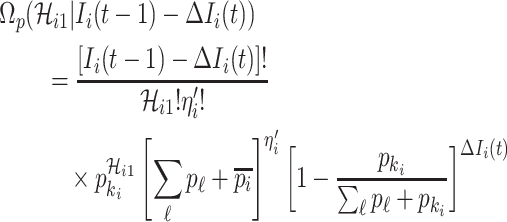where the last item on the RHS accounts for the probability that confirmed infected travelers all do not visit .

Taking into account all the above cases, the probability that infected hosts arrive at destination is measured by the following transferring estimator:

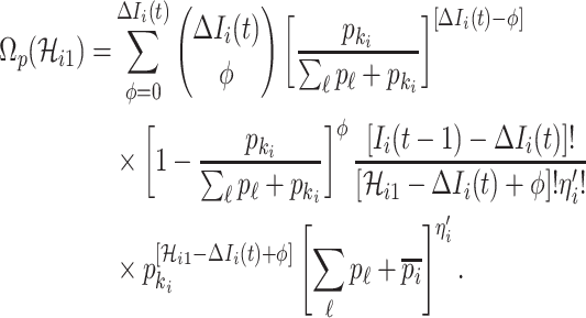Type 2: , i.e., the observed reduction in the number of infected hosts exceeds the number of infected hosts transferred to . Similar to the above analysis, we develop the transferring estimator by considering all possible cases that are in accordance with this condition.

If infected hosts transferred to are all from the observable travelers , the transferring estimator becomes

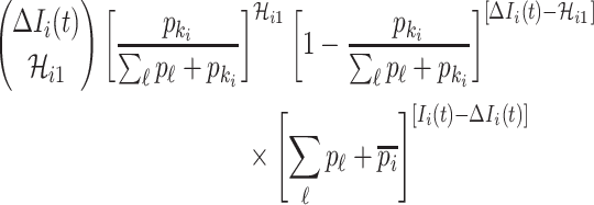where the last item accounts for the constraint that the remaining infected hosts will not be transferred to .

Similar to type 1, the other two cases are: only a fraction of infected hosts transferred to are from the observable travelers , and infected hosts transferred to are all not from the observable travelers , we can also derive the transferring estimators.

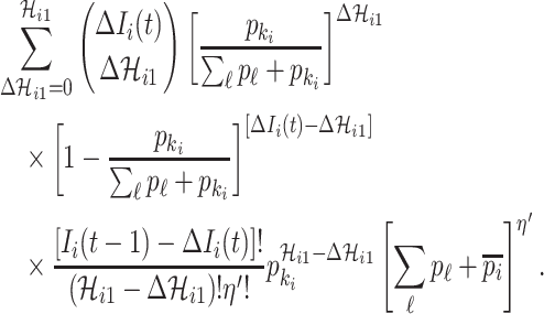
Taking into account all these cases, the probability that infected hosts move to the destination subpopulation is measured by the following transferring estimator:

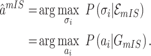
Generally, set consists of the three classes of subpopulations discussed above: unobservable subpopulation, partially observable subpopulation, and observable subpopulation of . According to (4), generally each potential pathway corresponds to a potential solution , the most-likely invasion pathway for a can be identified as

B. Case of

Finally, we consider the case of , which is more complicated than , because some infectious populations in set may have more than one invasion edge to the corresponding susceptible subpopulations in set , and the number of elements in set are more than one, which obey a joint probability distribution of transferring likelihood. As shown in Fig. 2, an INC includes set and . The first arrival infected individuals invaded each susceptible subpopulation in set are , respectively. Here, denote the subset of susceptible neighbor subpopulations in set of infected subpopulation , and the subset of infected neighbor subpopulations in set of susceptible subpopulation .

We define a potential solution for the , if subject to two conditions:

• 1)
  

  ;
• 2)for any which denotes the number of infected hosts travel to subpopulation from at , we have , where .

If a has potential solutions, let , .

Similarly, we first discuss the accurately identifiable pathway for a given , then estimate the most-likely numbers of each as accurate as possible by designing our identification algorithm, since one solution of (16) corresponds to one invasion pathway of an INC .

1). Accurate Identification of Invasion Pathway:

Given a few satisfied prerequisites, for all of the equations constituted by (16) can has a unique solution, which implies that the invasion pathway of that INC can be identified accurately. Theorem 2 elucidates this scenario.

Theorem 2 (Accurate Identification of Invasion Pathway):

With the following conditions: 1) the number of invasion edges ; 2) the neighbor subpopulations of each subpopulation in set are with the transition to or to except their neighbor subpopulations in set during to ; and 3) , the invasion pathway of an INC can be identified accurately.

Proof:

Since the number of infected individuals in the partially observable subpopulation reduces at time , i.e., and , it is inevitable that a few infected carries diffuse away from subpopulation . Occurring the state transitions of at time , subpopulations in the neighborhood of (excluding the new contaminated subpopulation ) cannot receive infected travelers. Therefore, the only possible destination for those infected travelers is subpopulation .

The conditions and make the equations and only has the unique solution . The reason is that rank , where is the coefficient matrix of equations and . Thus the invasion pathway of this can be identified accurately.

2). Potential Invasion Pathway:

If the conditions of Theorem 2 are unsatisfied, the equations constituted by (16) has multiple solutions, each solution corresponds to a set of potential invasion pathways that can result in the related . We derive the transferring likelihood of each potential solution similar to case of . Therefore, the likelihood of solution is characterized by

where represents the number of solution , and the last item represents the transferring estimator of infected subpopulation in , . Note that and correspond to a potential invasion pathway of and , respectively.

Now we discuss the transferring estimator of subpopulation according to its extent of subpopulation observability.

• 1)Subpopulation has only one neighbor (invasion edge) in set . In this case, the transferring estimator is the same as the depicted one in .
• 2)Subpopulation has neighbors (invasion edges) in set .

Suppose there are totally edges emanate from which consist of the following three kinds.

• 1)There are invasion edges (), labeled , along which the traveling rates are , and invade the subpopulations in the subset , respectively.
• 2)There are unobservable and partially observable edges, labeled , respectively. Along each unobservable or partially observable edge, the traveling rate is , , and infected hosts leave . Accordingly, in total infected hosts leave through the unobservable and partially observable edges.
• 3)There remain observable edges, labeled as , respectively. Along each observable edge, the traveling rate is ,, and infected hosts leave . With probability , an infected host keeps staying at the source . There are infected hosts staying in subpopulation with the probability . Because connects the unobservable and partially observable infected subpopulations, we only know the sum .

Now, we employ the following estimators to evaluate the transferring likelihood of the three categories of .

a). Unobservable subpopulation :

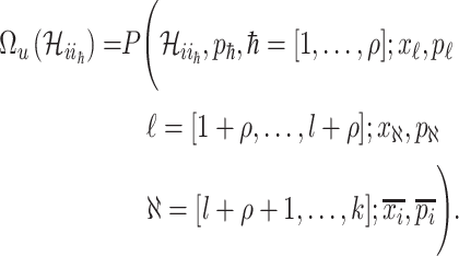
Because , we do not know whether and how many infected individuals travel to which destinations. Similar to the INC , the transferring likelihood estimator of is

By means of the observable edges, the transferring estimator can be simplified as

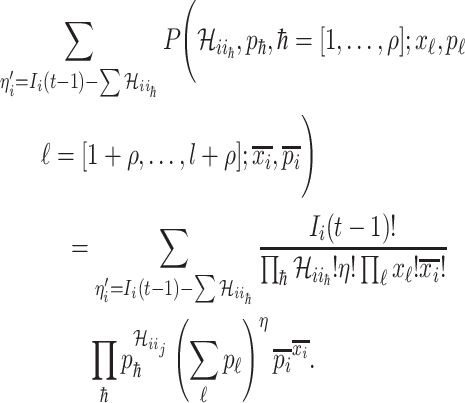Then the transferring estimator becomes by the marginal distribution as

b). Observable subpopulation ( to ):

For this situation, all come from . The transferring likelihood estimator of a observable subpopulation is

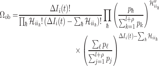where .

c). Partially observable subpopulation :

Due to , at least infected hosts leave source from to .

We first decompose as two subsets: and , , where . Denote the infected hosts coming from , and the infected hosts coming from . Then we analyze the transferring estimator on the following two types.

Type 1 (): Suppose , which represents the number of infected hosts coming from . Given a fixed , there may be more than one permutation for . The transferring likelihood estimator is

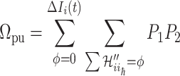where

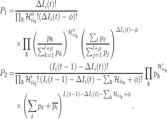Type 2 (): Suppose , which represents the number of infectious hosts coming from . Given a fixed , there may be more than one solution for . The transferring likelihood estimator is

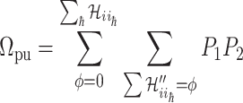where and are the same as those in (22).

According to (17), the most-likely invasion pathways for an INC can be identified as

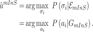Note that if the first arrival infectious individuals , there may be multiple potential solutions corresponding to one potential pathway. For example, a is illustrated in Fig. 4. In this situation, we merge the transferring likelihood of potential solutions of or if they belong to the same invasion pathways, then find out the most-likely invasion pathways, which are corresponding to the maximum transferring likelihood.

Fig. 4.

Example of INC. Suppose that three infected cases reach subpopulation simultaneously, which means . The three possible permutations are: ; ,; and . The permutations and indicate the same pathways, but is different.

According to (1) and (2), the whole invasion pathway can be reconstructed chronologically by assembling all identified invasion pathway of each INC after identification of four classes of INCs. To depict the IPI algorithm explicitly, the pseudocode for our algorithm is given in Algorithm 2.

Algorithm 2 IPI

• 1:Inputs: the time series of infection data and topology of network (including diffusion rates )
• 2:Find all invasion events via EAT data
• 3:for each invasion event
• 4:Invasion partition to find out the , , and .
• 5:for each or
• 6:if it satisfy conditions of Th 1 or Th 2
• 7:compute the unique invasion pathway
• 8:end if
• 9:if don’t satisfy conditions of Th 1 or Th 2 compute the all potential solutions
• 10:compute the or
• 11:merge the or of potential solution if they belong to same pathway
• 12:end if
• 13:end for
• 14:find the maximal and invasion pathway
• 15:end for
• 16:reconstruct the whole invasion pathways (T) by assembling each invasion cases chronologically

C. Analysis of IPI Algorithm

Science IPI algorithm is based on hierarchical-iteration-like decomposition technique, which reduce the temporal-spatial complexity of spreading, it can handle large-scale spatial pandemic. Note that the invasion infected hosts at EAT always are very small (generally ≤ 3). Therefore, the computation cost of our IPI algorithm is small, and we employ the enumeration algorithm to compute each of potential permutations. In this section, we only discuss the simplest situation that one pathway only corresponds to one permitted solution in an INC. The situation of one pathway corresponds to multiplex potential solutions can be extended.

Denote the probability corresponding to the most likely pathways for a given INC. Thus we have

Property 1:

Given an INC “” or “,” , there must exist and satisfying

Proof:

Suppose that , where is the number of potential solutions. Thus ; Because , let We have .

D. Identifiability of Invasion Pathway

Accordingly, our IPI algorithm first decomposes the whole invasion pathways into four classes of INCs. Some INCs are easy to identify, but some are difficult. Therefore, it is important to describe how possible an INC can be wrongly identified. The identification extent of an INC relates with the absolute value of and information given by the probability vector of all potential invasion pathways. We employ the entropy to describe the information of likelihood vector, which contains the all likelihood of potential solutions/pathways of an INC.

Definition 1 (Entropy of Transferring Likelihoods of Potential Solutions):

According to Shannon entropy, we define the normalized entropy of transferring likelihood as

This likelihood entropy tells the information embedded in the likelihood vector of the potential solutions of a given INC.

The bigger of and the smaller of entropy , the easier to identify the epidemic pathways for an INC. Define identifiability of invasion pathways to characterize the feasibility an INC can be identified

Although the likelihood entropies of some INCs are small (less than 0.5), they are still difficult to identify, because their are much less than 0.5. Therefore, identifiability describes the practicability of a given or better than only using or likelihoods entropy . The identifiability statistically tells us why some INCs are easy to identify, whose are more than 0.5, and why some INCs are difficult to identify, whose are much less than 0.5.

Next we show that there exist the upper and lower boundaries of identifiability for a given INC.

Theorem 3:

Given an INC “” or “,” is the identifiability computed by the IPI algorithm. There exist a lower boundary and an upper boundary that

where .

Proof:

, where . According to Fano’s inequality, the entropy .

On the other hand, we note that function is strictly convex. According to Jensen’s inequality, . . Therefore, , where and . That completes the proof of Theorem 3.

IV. Computational Experiments

To verify the performance of our algorithm, we proceed networked metapopulation-based Monte Carlo simulation method to simulate stochastic epidemic process on the AAN and the Barabasi–Albert (BA) networked metapopulation.

The AAN is a highly heterogeneous network. Each node of the AAN represents an airport, the population size of which is the serving area’s population of this airport. The directed traffic flow is the number of passengers through this edge/airline. The data of the AAN we are used to simulate is based on the true demography and traffic statistics [50]. We take the maximal component consisted of 404 nodes (airports/subpopulations) of all American airports as the network size of the ANN. The average degree of the AAN is nearly . The total population of the AAN is the , which covers most of the population of the USA.

The BA network obeys heterogeneous degree distribution [51], which holds two properties of growth and preference attachment. For a BA networked metapopulation, each node is a subpopulation containing many individuals. The details of how to generate a BA networked metapopulation including travel rates setting is presented in Appendix B. To test the performance of our algorithm to handle large-scale network, the subpopulations number of the BA networked metapopulation is fixed as 3000. This is nearly equal to the number of the world airports network [52]. We fix as the average degree of the BA networked metapopulation. The initial population size of each subpopulation is , and the total population is , which covers most of the active travelers of the world.

A. Networked Metapopulation-Based Monte Carlo Simulation Method to Simulate Stochastic Epidemic Process

At the beginning, we assume only one subpopulation is seeded as infected and others are susceptible. Thus , . We record and update each individual’s state (i.e., susceptible or infected) at each time step. At each ( is defined as the unit time from to ), the transmission rate and diffusion rate are converted into probabilities. The rules of individuals reaction and diffusion process in are as follows.

1). Reaction Process:

Individuals which are in the same subpopulation are homogeneously mixing. Each susceptible individual (in subpopulation ) becomes infected with probability . Therefore, the average number of newly added infected individuals is , but the simulation results fluctuate from one realization to another. The reaction process is simulated by binomial distribution.

2). Diffusion Process:

After reaction, the diffusion process of individuals between different subpopulation posterior to the reaction process is taken into account. Each individual from subpopulation migrates to the neighboring subpopulation with probability . The average number of new infectious travelers from subpopulation to is . The diffusion process is simulated by binomial distribution or multinomial distribution.

B. Numerical Results

We compared our IPI algorithm with three heuristic algorithms that generate the SPT or minimum spanning tree of the metapopulation networks.

• 1)Average-Arrival-Time (ARR)-Based SPT [30]: The minimum distance path from subpopulation to subpopulation over all possible paths is generated in terms of mean first arrival time. Thus the average-arrival-time-based SPT is constructed by assembling all shortest paths from the seed subpopulation to other subpopulations of the whole network.
• 2)Effective (EFF)-Distance-Based Most Probable Paths Tree [4] Methods: From subpopulation to subpopulation , the effective distance is defined as the minimum of the sum of effective lengths along the arbitrary legs of the path. The set of shortest paths to all subpopulations from seed subpopulation constitutes an SPT.
• 3)Monte Carlo-Maximum-Likelihood (MCML)-Based Most Likely Epidemic Invasion Tree [43]: To produce a most likely infection tree, they constructed the minimum spanning tree from the seed subpopulation to minimize the distance. Some recent works [53]–[55] uses machine learning or genetic algorithms to infer transmission networks from surveillance data. Because of the distinction in model assumptions and conditions, we do not perform comparison with them.

We consider to access the identification accuracy for the inferred invasion pathways. This accuracy is defined by the ratio between the number of corrected identified invasion pathways by each method and the number of true invasion pathways, respectively. We also compute the accuracy of accumulative INCs of and . This accuracy is defined by the ratio between the number of corrected identified invasion pathways by each method in this class of INC and the number of true invasion pathways in this classes of INC. Additionally, we investigate the identification accuracy of early stage of a global pandemic spreading, which is important to help understand how to predict and control the prevalence of epidemics.

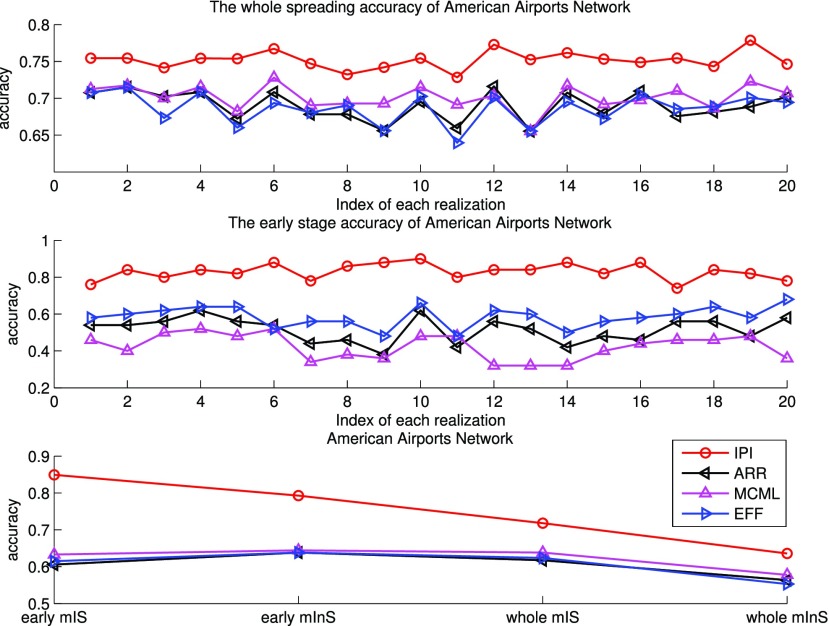
In Fig. 5 (top and middle), we observe the whole identification accuracy and the early-stage identification accuracy. Fig. 5 (bottom) shows the early and whole accumulative identification accuracy of and through 20 independent realizations on the AAN for each algorithm, respectively. The simulation results show our algorithm is outperformance, which indicates heterogeneity of structure of the AAN plays an important role.

Fig. 5.

Top and middle: identified accuracy for the whole and early stage (before appearance of the first 50 infected subpopulations) invasion pathways for 20 independent spreading realizations on the AAN. Bottom: accumulative identified accuracy of INCs ( and ) for the early stage and the whole invasion pathways on the AAN.

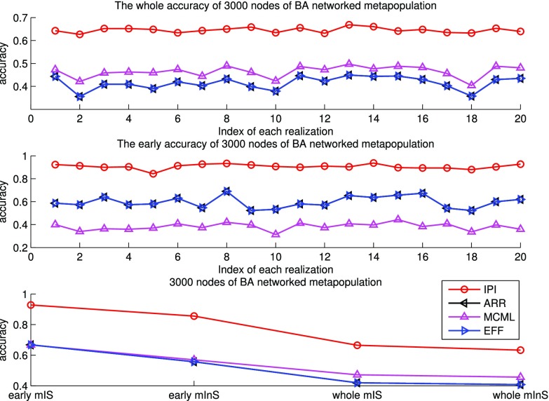
Fig. 6 shows the results of the BA networked metapopulation with 3000 subpopulations, the top of which presents the identification accuracy of whole invasion pathway for each realization of the four algorithms, while Fig. 6 (middle) shows the identification accuracy of early stage invasion pathway for each realization. Fig. 6 (bottom) shows accumulative identified accuracy of and of 20 realizations for four algorithms respectively. The simulation results indicate that our algorithm can handle a large scale networked metapopulation with robust performance. 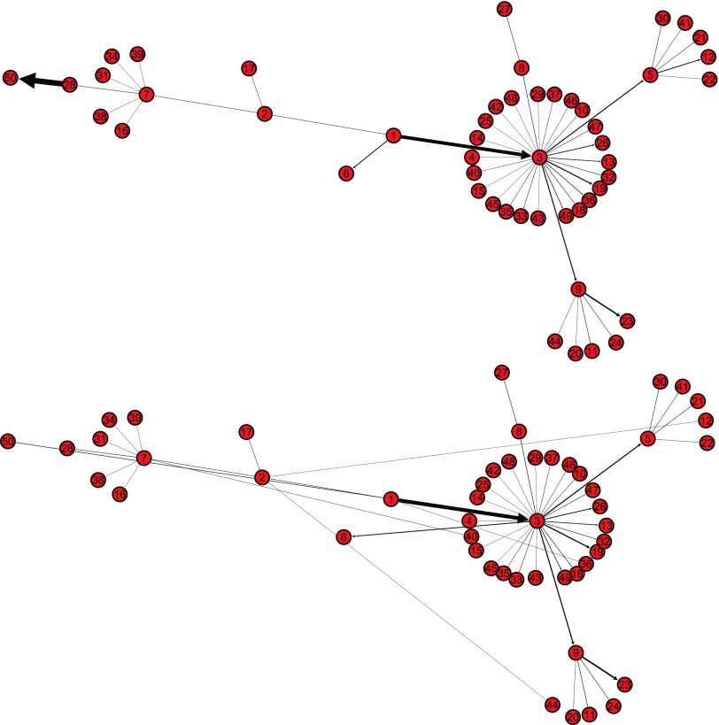Note that the performance of the ARR for the BA networked metapopulation is the same as that of the EFF, because our parameter is a constant in the diffusion model (see Appendix B). Fig. 7 shows the comparison of the actual invasion pathways and the most likely identified invasion pathways for a given realization, during the early stage on the AAN.

Fig. 6.

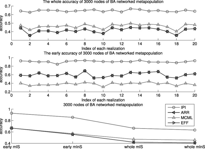
Top and middle: identified accuracy for the whole and early stage invasion pathways for 20 independent spreading realizations on 3000 subpopulations of the BA networked metapopulation. Bottom: accumulative identified accuracy of and for the early stage (the first 300 infected subpopulations) and the whole invasion pathways on 3000 subpopulations of the BA networked metapopulation.

Fig. 7.

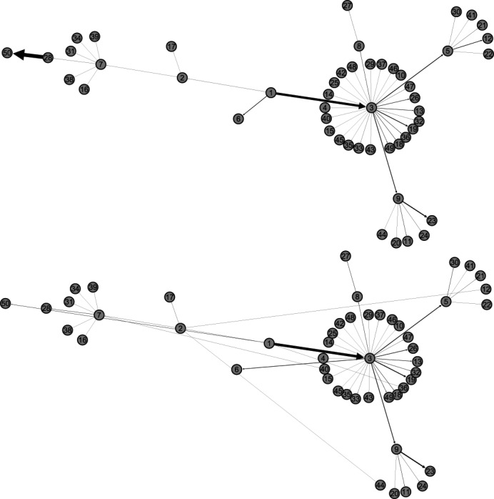
Illustration of the actual invasion pathways and the most likely identified invasion pathways, in a given realization, during the early stage (before the appearance of 50 infected subpopulations) on the AAN. Subpopulation 1 is the seed.

The numerical results suggest that networks with different topologies yield different identification performances, which indicate an identification algorithm should embed in both effects of spreading and topology. Our algorithm takes into account both heterogeneity of epidemics (the number of infected individuals) and network topology (diffusion flows).

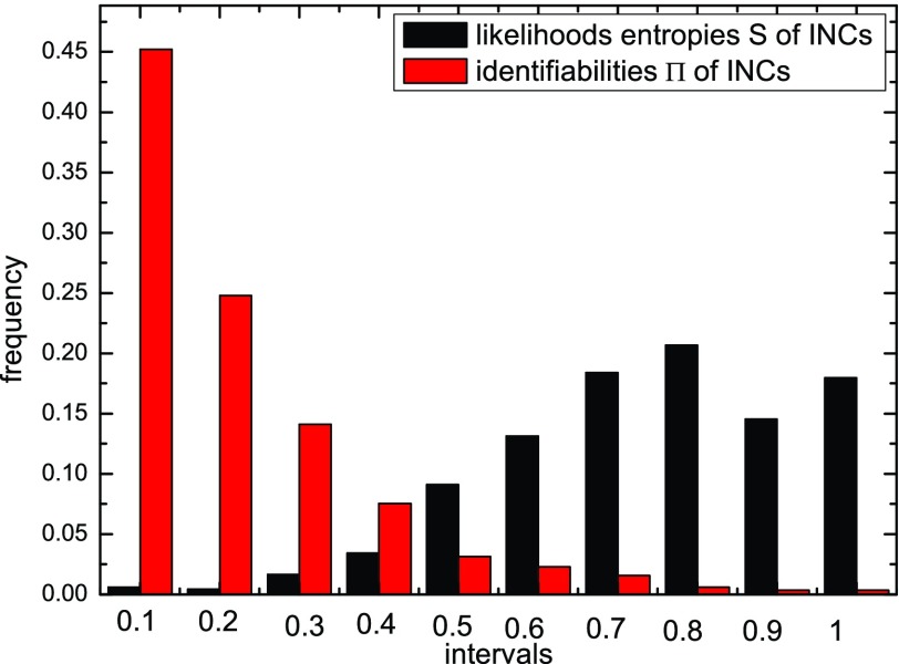
We finally test the identifiability of an INC. Fig. 8 shows the entropy and identifiability of wrongly identified of 20 realizations on the AAN. The smaller the identifiability of an INC is, the easier it is prone to be wrongly identified. The identifiability depicts the wrongly identified more reasonable than the likelihoods entropy. It indicates that identifiability has a better performance to distinguish whether an INC is difficult to identify or not than using the likelihoods entropy.

Fig. 8.

Statistics analysis of the likelihoods entropy and identifiability of wrongly identified of 20 realizations of epidemic spreading on the AAN.

V. Conclusion

To conclude, we have proposed an identification framework as the so called IPI algorithm to explore the problem of inferring invasion pathway for a pandemic outbreak. We first anatomize the whole invasion pathway into four classes of INCs at each EAT. Then we identify four classes of INCs, and reconstruct the whole invasion pathway from the source subpopulation of a spreading process. We introduce the concept of identifiability to quantitatively analyze the difficulty level that an INC can be identified. The simulation results on the AAN and large-scale BA networked metapopulation have demonstrated our algorithm held a robust performance to identify the spatial invasion pathway, especially for the early stage of an epidemic. We conjecture the proposed IPI algorithm framework can extend to the problems of virus diffusion in computer network, human to human’s epidemic contact network, and the reaction dynamics may extend to the susceptible-infected-removed or susceptible-infected-susceptible dynamics.

Biographies

Jian-Bo Wang (S’15) received the B.Eng. degree in electronic science and technology from the Hefei University of Technology, Hefei, China, in 2005, and the M.Sc. degree in system theory from the University of Shanghai for Science and Technology, Shanghai, China, in 2010. He is currently pursuing the Ph.D. degree in circuits and systems with the Department of Electronic Engineering, Fudan University, Shanghai.

His current research interests include modeling and analyzing the spatial spread of emerging infectious diseases, statistics, optimization, and network science.

Mr. Wang was a recipient of the Fudan University Excellent Doctoral Research Program (985 Program) in 2013, the Excellent Master Dissertation Award of Shanghai Municipality in 2012, and the Outstanding University Graduates from Shanghai Municipal Government in 2010.

Lin Wang (M’14) received the B.Sc. degree in applied physics from the Department of Physics, Southeast University, Nanjing, China, in 2006, the M.Sc. degree in theoretical physics from the School of Physics, Nankai University, Tianjin, China, in 2009, and the Ph.D. degree in circuits and systems from the Department of Electronic Engineering, Fudan University, Shanghai, China, in 2013.

He is currently a Post-Doctoral Fellow with the WHO Collaborating Centre for Infectious Disease Epidemiology and Control, School of Public Health, Li Ka Shing Faculty of Medicine, University of Hong Kong, Hong Kong. His current research interests include mathematical and statistical epidemiology, infectious diseases modeling, stochastic processes, decision and optimization, self-organizing, and networking systems.

Dr. Wang was a recipient of the Excellent Doctoral Dissertation Award of Shanghai Municipality in 2015, the Outstanding University Graduates from Shanghai Municipal Government in 2013, and the Best Student Paper Award in Seventh Chinese Conference on Complex Networks in 2011. He serves as a Reviewer for about 20 journals and IEEE Transactions.

Xiang Li (M’05–SM’08) received the B.Sc. and Ph.D. degrees in control theory and control engineering from Nankai University, Tianjin, China, in 1997 and 2002, respectively.

He was with the International University of Bremen, Bremen, Germany, and Shanghai Jiao Tong University, Shanghai, China, as a Humboldt Research Fellow in 2005 and 2006 and an Associate Professor from 2004 to 2007. He joined Fudan University, Shanghai, China, as a Professor of Electronic Engineering in 2008. He served as the Head of the Electronic Engineering Department, Fudan University, in 2010–2015. He is the Founding Director of the Research Center of Smart Networks and Systems, School of Information Science and Engineering, Fudan University. He has (co-)authored four research monographs and over 200 peer-refereed publications in journals and conferences. His current research interests include theories and applications of complex network and network science.

Prof. Li was a recipient of the National Science Foundation for Distinguished Young Scholar of China in 2014, the Shanghai Science and Technology Young Talents Award in 2010, the Shanghai Natural Science Award (First Class) in 2008, and the IEEE Guillemin-Cauer Best Transactions Paper Award from the IEEE Circuits and Systems Society in 2005. He serves and served as an Associate Editor for the IEEE Transactions on Circuits and Systems—I: Regular Papers, the IEEE Circuits and Systems Society Newsletter, and Control Engineering Practice, and a Guest Associate Editor of the International Journal of Bifurcations and Chaos.

Appendix A. Mobility Operator

We discuss the individual mobility operator. Due to the presence of stochasticity and independence of individual mobility, the number of successful transform of individuals between or among adjacent subpopulations is quantified by a binomial or a multinomial process, respectively. If the focal subpopulation only has one neighboring subpopulation , the number of individuals in a given compartment ( and ) transferred from to per unit time, , is generated from a binomial distribution with probability representing the diffusion rate and the number of trials , that is

If the focal subpopulation has multiple neighboring subpopulations , with representing ’s degree, the numbers of individuals in a given compartment transferred from to are generated from a multinomial distribution with probabilities () representing the diffusion rates on the edges emanated from subpopulation and the number of trails , that is

where .

Appendix B. Generic Diffusion Model to Generate Barabasi–Albert Metapopulation Network

We develop a general diffusion model to generate a BA metapopulation network in Section V, which characterizes the human mobility pattern on the empirical statistical rules of air transportation networks.

The diffusion rate from subpopulation to is , where denotes the traffic flow from subpopulation to . These empirical statistical rules are verified in the air transportation network [52]: .

All the above empirical formulas relate to node’s degree . To generate an artificial transportation network, we introduce a generic diffusion model to determine the diffusion rate

where stands for the elements of the adjacency matrix ( if connects to , and otherwise), is a constant, and is a variable parameter. We assume that parameter follows the Gaussian distribution . Based on the empirical rule of , where is approximately linear with , the least squares estimation is employed to evaluate parameters and if we set the initial population of each node and constant . Then, for a given BA network, we get a BA networked metapopulation in which real statistic information is embedded by using the above method.

Funding Statement

This work was supported in part by the National Science Fund for Distinguished Young Scholars of China under Grant 61425019, the National Natural Science Foundation under Grant 61273223, and the “Shu Guang“ project supported by Shanghai Municipal Education Commission and Shanghai Education Development Foundation under Grant 14SG03. The work of J.-B. Wang and L. Wang was in part supported by the Fudan University Excellent Doctoral Research Program (985 Program).

References

- [1].Keeling M. J. and Rohani P., Modeling Infectious Diseases in Humans and Animals. Princeton, NJ, USA: Princeton Univ. Press, 2008. [Google Scholar]
- [2].Heesterbeek H., et al. , “Modeling infectious disease dynamics in the complex landscape of global health,” Science, vol. 347, no. 6227, pp. 1–10, Mar. 2015. [DOI] [PMC free article] [PubMed] [Google Scholar]
- [3].Fitch J. P., “Engineering a global response to infectious diseases,” Proc. IEEE, vol. 103, no. 2, pp. 263–272, Feb. 2015. [DOI] [PMC free article] [PubMed] [Google Scholar]
- [4].Brockmann D. and Helbing D., “The hidden geometry of complex, network-driven contagion phenomena,” Science, vol. 342, no. 6164, pp. 1337–1342, Dec. 2013. [DOI] [PubMed] [Google Scholar]
- [5].McMichael A. J., “Globalization, climate change, and human health,” New England J. Med., vol. 368, no. 14, pp. 1335–1343, Apr. 2013. [DOI] [PubMed] [Google Scholar]
- [6].Mclean A. R., May R. M., Pattison J., and Weiss R. A., Eds., SARS: A Case Study in Emerging Infections. New York, NY, USA: Oxford Univ. Press, 2005. [Google Scholar]
- [7].Fraser C., et al. , “Pandemic potential of a strain of influenza A (H1N1): Early findings,” Science, vol. 324, no. 5934, pp. 1557–1561, Jun. 2009. [DOI] [PMC free article] [PubMed] [Google Scholar]
- [8].Yang Y., et al. , “The transmissibility and control of pandemic influenza A (H1N1) virus,” Science, vol. 326, no. 5953, pp. 729–733, Oct. 2009. [DOI] [PMC free article] [PubMed] [Google Scholar]
- [9].Yu H., et al. , “Human infection with avian influenza A H7N9 virus: An assessment of clinical severity,” Lancet, vol. 382, no. 9887, pp. 138–145, Jun. 2013. [DOI] [PMC free article] [PubMed] [Google Scholar]
- [10].Lam T. T.-Y., et al. , “Dissemination, divergence and establishment of H7N9 influenza viruses in China,” Nature, vol. 522, pp. 102–105, Jun. 2015. [DOI] [PubMed] [Google Scholar]
- [11].Gomes M. F. C., et al. , “Assessing the international spreading risk associated with the 2014 West African Ebola outbreak,” PLoS Currents Outbreaks, vol. 6, Sep. 2014. Doi: 10.1371/currents.outbreaks.cd818f63d40e24aef769dda7df9e0da5. [DOI] [PMC free article] [PubMed] [Google Scholar]
- [12].Cowling B. J., et al. , “Preliminary epidemiological assessment of MERS-CoV outbreak in South Korea, May to June,” Eurosurveillance, vol. 20, no. 25, pp. 7–13, Jun. 2015. [DOI] [PMC free article] [PubMed] [Google Scholar]
- [13].Wang X. and Chen G., “Complex network: Small-world, scale-free, and beyond,” IEEE Circuits Syst. Mag., vol. 3, no. 1, pp. 6–20, Jan-Mar 2003. [Google Scholar]
- [14].Newman M. E. J., Networks: An Introduction. New York, NY, USA: Oxford Univ. Press, 2010. [Google Scholar]
- [15].Tan C. W., Chiang M., and Srikant R., “Fast algorithms and performance bounds for sum rate maximization in wireless networks,” IEEE/ACM Trans. Netw., vol. 21, no. 3, pp. 706–719, Jun. 2013. [Google Scholar]
- [16].Yang B., Liu J., and Liu D., “Characterizing and extracting multiplex patterns in complex networks,” IEEE Trans. Syst., Man, Cybern. B, Cybern., vol. 42, no. 2, pp. 469–481, Apr. 2012. [DOI] [PubMed] [Google Scholar]
- [17].Fu X., Small M., and Chen G., Propagation Dynamics on Complex Networks: Models, Methods and Stability Analysis. New York, NY, USA: Wiley, 2013. [Google Scholar]
- [18].Pastor-Satorras R., Castellano C., Van Mieghem P., and Vespignani A., “Epidemic processes in complex networks,” Rev. Mod. Phys., vol. 87, no. 3, pp. 925–979, Jul-Sep 2015. [Google Scholar]
- [19].Wang L. and Li X., “Spatial epidemiology of networked metapopulation: An overview,” Chin. Sci. Bull., vol. 59, no. 28, pp. 3511–3522, Jul. 2014. [DOI] [PMC free article] [PubMed] [Google Scholar]
- [20].Chen P.-Y., Cheng S.-M., and Chen K.-C., “Optimal control of epidemic information dissemination over networks,” IEEE Trans. Cybern., vol. 44, no. 12, pp. 2316–2328, Dec. 2014. [DOI] [PubMed] [Google Scholar]
- [21].Griffin C. and Brooks R., “A note on the spread of worms in scale-free networks,” IEEE Trans. Syst., Man, Cybern. B, Cybern., vol. 36, no. 1, pp. 198–202, Feb. 2006. [DOI] [PubMed] [Google Scholar]
- [22].Chen L.-C. and Carley K. M., “The impact of countermeasure propagation on the prevalence of computer viruses,” IEEE Trans. Syst., Man, Cybern. B, Cybern., vol. 34, no. 2, pp. 823–833, Apr. 2004. [DOI] [PubMed] [Google Scholar]
- [23].Balcan D., et al. , “Seasonal transmission potential and activity peaks of the new influenza A(H1N1): A Monte Carlo likelihood analysis based on human mobility,” BMC Med., vol. 7, no. 45, pp. 1–12, Sep. 2009. [DOI] [PMC free article] [PubMed] [Google Scholar]
- [24].Ferguson N. M., et al. , “Strategies for mitigating an influenza pandemic,” Nature, vol. 442, no. 7101, pp. 448–452, Jul. 2006. [DOI] [PMC free article] [PubMed] [Google Scholar]
- [25].Colizza V., Barrat A., Barthelemy M., Valleron A. J., and Vespignani A., “Modeling the worldwide spread of pandemic influenza: Baseline case and containment interventions,” PLoS Med., vol. 4, no. 1, pp. 95–110, Jan. 2007. [DOI] [PMC free article] [PubMed] [Google Scholar]
- [26].Wang L., Zhang Y., Huang T., and Li X., “Estimating the value of containment strategies in delaying the arrival time of an influenza pandemic: A case study of travel restriction and patient isolation,” Phys. Rev. E, vol. 86, no. 3, Sep. 2012, Art. ID 032901. [DOI] [PubMed] [Google Scholar]
- [27].Halloran M. E., et al. , “Modeling targeted layered containment of an influenza pandemic in the United States,” Proc. Nat. Acad. Sci. USA, vol. 105, no. 12, pp. 4639–4644, Mar. 2008. [DOI] [PMC free article] [PubMed] [Google Scholar]
- [28].Wu J. T., Leung G. M., Lipsitch M., Cooper B. S., and Riley S., “Hedging against antiviral resistance during the next influenza pandemic using small stockpiles of an alternative chemotherapy,” PLoS Med., vol. 6, no. 5, pp. 1–11, May 2009. [DOI] [PMC free article] [PubMed] [Google Scholar]
- [29].Lofgren E. T., et al. , “Opinion: Mathematical models: A key tool for outbreak response,” Proc. Nat. Acad. Sci. USA, vol. 111, no. 51, pp. 18095–18096, Dec. 2014. [DOI] [PMC free article] [PubMed] [Google Scholar]
- [30].Gautreau A., Barrat A., and Barthélemy M., “Global disease spread: Statistics and estimation of arrival times,” J. Theor. Biol., vol. 251, no. 3, pp. 509–522, Apr. 2008. [DOI] [PubMed] [Google Scholar]
- [31].Miao H., Xia X., Perelson A. S., and Wu H., “On identifiability of nonlinear ODE models and applications in viral dynamics,” SIAM Rev., vol. 53, no. 1, pp. 3–39, Feb. 2011. [DOI] [PMC free article] [PubMed] [Google Scholar]
- [32].Shah D. and Zaman T., “Rumors in a network: Who’s the culprit?” IEEE Trans. Inf. Theory, vol. 57, no. 8, pp. 5163–5181, Aug. 2011. [Google Scholar]
- [33].Luo W., Tay W. P., and Leng M., “Identifying infection sources and regions in large networks,” IEEE Trans. Signal Process., vol. 61, no. 11, pp. 2850–2865, Jun. 2013. [Google Scholar]
- [34].Wang Z., Dong W., Zhang W., and Tan C. W., “Rumor source detection with multiple observations: Fundamental limits and algorithms,” in Proc. ACM SIGMETRICS, Austin, TX, USA, Jun. 2014, pp. 1–13. [Google Scholar]
- [35].Dong W., Zhang W., and Tan C. W., “Rooting out the rumor culprit from suspects,” in Proc. IEEE Int. Symp. Inf. Theory (ISIT), Istanbul, Turkey, Jul. 2013, pp. 2671–2675. [Google Scholar]
- [36].Wang Z., Dong W., Zhang W., and Tan C. W., “Rooting our rumor sources in online social networks: The value of diversity from multiple observations,” IEEE J. Sel. Topics Signal Process., vol. 9, no. 4, pp. 663–677, Jun. 2015. [Google Scholar]
- [37].Han X., Shen Z., Wang W.-X., and Di Z., “Robust reconstruction of complex networks from sparse data,” Phys. Rev. Lett., vol. 114, no. 2, Jan. 2015, Art. ID 028701. [DOI] [PubMed] [Google Scholar]
- [38].Gomez-Rodriguez M., Leskovec J., and Krause A., “Inferring networks of diffusion and influence,” in Proc. 16th ACM SIGKDD Conf. Knowl. Disc. Data Mining (KDD), Washington, DC, USA, Jul. 2010, pp. 1019–1028. [Google Scholar]
- [39].Gomez-Rodriguez M., Leskovec J., and Krause A., “Inferring networks of diffusion and influence,” ACM Trans. Knowl. Disc. Data, vol. 5, no. 4, pp. 1–37, Feb. 2012. [Google Scholar]
- [40].Gomez-Rodriguez M., Balduzzi D., and Schölkopf B., “Uncovering the temporal dynamics of diffusion networks,” in Proc. 28th Int. Conf. Mach. Learn. (ICML), Bellevue, WA, USA, Jul. 2011, pp. 561–568. [Google Scholar]
- [41].Gomez-Rodriguez M., Leskovec J., Balduzzi D., and Schölkopf B., “Uncovering the structure and temporal dynamics of information propagation,” Netw. Sci., vol. 2, no. 1, pp. 26–65, Apr. 2014. [Google Scholar]
- [42].Daneshmand H., Gomez-Rodriguez M., Song L., and Schölkopf B., “Estimating diffusion network structures: Recovery conditions, sample complexity & soft-thresholding algorithm,” in Proc. 31st Int. Conf. Mach. Learn. (ICML), vol. 32 Beijing, China, Jun. 2014, pp. 793–801. [PMC free article] [PubMed] [Google Scholar]
- [43].Balcan D., et al. , “Multiscale mobility networks and the spatial spreading of infectious diseases,” Proc. Nat. Acad. Sci. USA, vol. 106, no. 51, pp. 21484–21489, Dec. 2009. [DOI] [PMC free article] [PubMed] [Google Scholar]
- [44].Tsui K.-L., Wong Z. S.-Y., Goldsman D., and Edesess M., “Tracking infectious disease spread for global pandemic containment,” IEEE Intell. Syst., vol. 28, no. 6, pp. 60–64, Nov-Dec 2013. [Google Scholar]
- [45].Barthélemy M., “Spatial networks,” Phys. Rep., vol. 499, nos. 1–3, pp. 1–101, Feb. 2010. [Google Scholar]
- [46].Bazzani A., Giorgini B., Rambaldi S., Gallotti R., and Giovannini L., “Statistical laws in urban mobility from microscopic GPS data in the area of Florence,” J. Stat. Mech., vol. 2010, no. 5, May 2010, Art. ID P05001. [Google Scholar]
- [47].Peng C., Jin X., Wong K.-C., Shi M., and Liò P., “Collective human mobility pattern from taxi trips in urban area,” PLoS ONE, vol. 7, no. 4, Apr. 2012, Art. ID e34487. [DOI] [PMC free article] [PubMed] [Google Scholar]
- [48].Liang X., Zhao J., Dong L., and Xu K., “Unraveling the origin of exponential law in intra-urban human mobility,” Sci. Rep., vol. 3, Oct. 2013, Art. ID 2983. [DOI] [PMC free article] [PubMed] [Google Scholar]
- [49].Brooks-Pollock E., Roberts G. O., and Keeling M. J., “A dynamic model of bovine tuberculosis spread and control in Great Britain,” Nature, vol. 511, no. 7508, pp. 228–231, Jul. 2014. [DOI] [PubMed] [Google Scholar]
- [50].Wang L., Li X., Zhang Y.-Q., Zhang Y., and Zhang K., “Evolution of scaling emergence in large-scale spatial epidemic spreading,” PLoS ONE, vol. 6, no. 7, Jul. 2011, Art. ID e21197. [DOI] [PMC free article] [PubMed] [Google Scholar]
- [51].Albert R. and Barabasi A.-L., “Statistical mechanics of complex networks,” Rev. Mod. Phys., vol. 74, no. 1, pp. 47–97, Jan. 2002. [Google Scholar]
- [52].Barrat A., Barthélemy M., Pastor-Satorras R., and Vespignani A., “The architecture of complex weighted networks,” Proc. Nat. Acad. Sci. USA, vol. 101, no. 11, pp. 3747–3752, Mar. 2004. [DOI] [PMC free article] [PubMed] [Google Scholar]
- [53].Wan X., Liu J., Cheung W.-K., and Tong T., “Inferring epidemic network topology from surveillance data,” PLoS ONE, vol. 9, no. 6, Jun. 2014, Art. ID e100661. [DOI] [PMC free article] [PubMed] [Google Scholar]
- [54].Shi B., Liu J., Zhou X.-N., and Yang G.-J., “Inferring plasmodium vivax transmission networks from tempo-spatial surveillance data,” PLoS Negl. Trop. Dis., vol. 8, no. 2, Feb. 2014, Art. ID e2682. [DOI] [PMC free article] [PubMed] [Google Scholar]
- [55].Yang X., Liu J., Zhou X.-N., and Cheung W.-K., “Inferring disease transmission networks at a metapopulation level,” Health Inf. Sci. Syst., vol. 2, no. 8, Nov. 2014. Art. ID PMC4375841. [DOI] [PMC free article] [PubMed] [Google Scholar]