A Darwinian Uncertainty Principle

Abstract

Reconstructing ancestral characters and traits along a phylogenetic tree is central to evolutionary biology. It is the key to understanding morphology changes among species, inferring ancestral biochemical properties of life, or recovering migration routes in phylogeography. The goal is 2-fold: to reconstruct the character state at the tree root (e.g., the region of origin of some species) and to understand the process of state changes along the tree (e.g., species flow between countries). We deal here with discrete characters, which are “unique,” as opposed to sequence characters (nucleotides or amino-acids), where we assume the same model for all the characters (or for large classes of characters with site-dependent models) and thus benefit from multiple information sources. In this framework, we use mathematics and simulations to demonstrate that although each goal can be achieved with high accuracy individually, it is generally impossible to accurately estimate both the root state and the rates of state changes along the tree branches, from the observed data at the tips of the tree. This is because the global rates of state changes along the branches that are optimal for the two estimation tasks have opposite trends, leading to a fundamental trade-off in accuracy. This inherent “Darwinian uncertainty principle” concerning the simultaneous estimation of “patterns” and “processes” governs ancestral reconstructions in biology. For certain tree shapes (typically speciation trees) the uncertainty of simultaneous estimation is reduced when more tips are present; however, for other tree shapes it does not (e.g., coalescent trees used in population genetics).

Reconstruction of the past is central to evolutionary biology (Maddison 1994; Felsenstein 2004; Liberles 2007). A first step is often phylogenetic reconstruction, which is central to understanding the origin, evolution and classification of species, protein families, and pathogens such as HIV, as well as for reconstructing the evolution of communities and ecosystems. However, phylogeny is not an end in itself; it is generally the support for more complete studies. In particular, one frequently reconstructs the evolution along a phylogenetic tree of ancestral characters of diverse nature, for example: molecular (Grass Phylogeny Working Group II 2012; Werner et al. 2014), phenotypic (Marazzi et al. 2012; Beaulieu et al. 2013), geographical (Lemey et al. 2009; Edwards et al. 2011; Lemey et al. 2014; Heintzman et al. 2016; Dudas et al. 2017), or ecological (Grass Phylogeny Working Group II 2012; Marazzi et al. 2012; Werner et al. 2014), and these reconstructions involve differing time scales, ranging from a few years for fast evolving viruses (e.g., Ebola, Dudas et al. 2017), to hundreds of millions years for higher eukaryotes (e.g., plants, Grass Phylogeny Working Group II 2012; Marazzi et al. 2012; Beaulieu et al. 2013; Werner et al. 2014). The problem has two facets (Fig. 1), which are generally combined: one may want to infer the “pattern,” that is, the ancestral states associated with phylogeny root and nodes, for example, the origin and migration routes of a species (Edwards et al. 2011; Heintzman et al. 2016) or an epidemic (Lemey et al. 2014; Dudas et al. 2017); or one may aim to understanding the “process” driving the character evolution and state changes such as the factors explaining the spread and sustainability of epidemics (Dudas et al. 2017), or the selection mechanisms acting at a molecular level (Lemey et al. 2012).

Figure 1.

Evolutionary process and history: a) Simple 2-state Markovian evolutionary process, where swaps into with rate and vice versa. This process has three (nonindependent) parameters: the state equilibrium frequencies ( and ) and the global rate of evolution (). b) This simple process acts along a phylogenetic tree, starting from the tree root with state and evolving the character state until the tree leaves, where various state values are observed. This observation (along with the phylogenetic tree) is all that is known. The goal is to estimate both the evolutionary pattern, notably the root state, and the parameters of the process. c) A more complex 4-state process, where the rate of change depends on the origin state, and not-only on the destination state. In this phylogeographic example, movement between four countries distributed across two continents moves at rates that are different (typically higher) within continents than between continents as indicated by the parameter . This model is formally equivalent to the HKY model of nucleotide substitution (with equal to , respectively), in which corresponds to the transition/transversion ratio. corresponds to the “equal-input” model (F81 with DNA).

Many methods have been proposed to reconstruct the pattern. Today, one most often uses probabilistic methods based on Markovian evolutionary models with numerical parameters to be estimated from the data (Maddison 1994; Felsenstein 2004; Liberles 2007). These models and their parameters are mathematical representations of the evolutionary processes. We deal here with discrete “unique” characters (e.g., a particular geographical or morphological character) as opposed to sequence characters (nucleotide or amino-acid). In this framework, we show, using information theory, mathematics and simulations, that evolutionary patterns (ancestral states) and processes (transition rates) cannot generally be simultaneously reconstructed with high accuracy from extant data. This result applies even to the simplest models, and to characters commonly used in a number of current studies, to describe a wide range of evolutionary phenomena, from molecular to ecological levels.

The Markovian evolutionary models used to reconstruct character evolution can be very simple, typically symmetrical with very few states (Fig. 1), but the current trend is to rely on ever more complex models which can be nonsymmetrical, with dozens of states (Dudas et al. 2017) (and therefore hundreds of parameters), latent variables (Marazzi et al. 2012) and, for some models, evolution over time (Lemey et al. 2009; Beaulieu et al. 2013; Heintzman et al. 2016; Dudas et al. 2017). The estimation of these models is based on maximum likelihood (ML) and Bayesian approaches, and the task is complicated by the fact that with unique characters there is only one realization of the process, corresponding to the state values observed at the leaves of the tree. Estimations are much simpler with DNA or protein sequences, where we assume the same model for all the characters (or for large classes of characters with site-dependent models) and thus benefit from multiple information sources. To learn the most complex of these (single-character) models, one can rely on user-supplied “factors,” such as the degree of connectivity between two countries in phylogeography (Lemey et al. 2014; Dudas et al. 2017). In a Bayesian framework, the parameters of complex models are sometimes viewed as nuisance parameters, and then the focus is not on their precise values, but on the global impact of the model on the reconstruction of the ancestral character states. To predict ancestral states, one generally uses marginal, joint or posterior likelihoods of the tree node states (Maddison 1994; Felsenstein 2004; Liberles 2007; Yang 2007; Matsumoto et al. 2015; Arenas et al. 2017). These two components (model estimation and ancestral reconstruction) are most often simultaneous and interdependent because neither the model nor the ancestral states are generally known (exceptions are paleontological rests with morphological characters, ancient DNA, and serial sampling over time of fast evolving organisms such as viruses). Only the tree and branch lengths can be considered as known; in practice, they are usually estimated from DNA or protein sequences via a probabilistic approach that includes the estimation of a model of site substitution for those sequences, and possibly a molecular clock model to date the tree nodes and root age (Felsenstein 2004). Note that the model used to estimate the tree and its branch lengths from sequences cannot describe the transition rates of the unique character (e.g., morphological or geographical) under study. For example, assuming that the tree is time scaled, we need to estimate the global rate of state changes per year (among other parameters, depending on the character evolution model), and this global rate cannot be deduced from the sequences.

Theoretical work has shown the difficulty of reconstructing ancestral states even when the evolutionary model describing the state changes is fully known (Evans et al. 2000; Mossel and Peres 2003; Gascuel and Steel 2010). If the rate of changes is too fast, the information provided by tree leaves is low and it is impossible to reconstruct the root state accurately, regardless of the estimation method. Note, however, that the reconstruction of states at recent tree nodes is easier, and can be achieved even when the root state cannot be reconstructed (Gascuel and Steel 2014). To our knowledge, there is no theoretical work on the joint estimation of evolutionary model parameters and the ancestral states, in standard models of character evolution. Moreover, very few simulations have been performed to verify that the complex models used in recent studies described in the previous paragraph could be estimated with high reliability. We show here that it is usually not possible to accurately reconstruct both the root character state and estimate the parameters of the evolutionary model. Intuitively, if the global rate of change is low, the reconstruction of the root is easy because the root state is largely preserved along the tree branches all the way to the leaves, but then they are too few state changes to accurately estimate the relative rates of changes from one state to another; conversely, with a rapid evolution, one cannot reconstruct the tree root, but estimating the rates seems easier.

While these intuitive trends are easily grasped, our aim in this article is to make these vague claims precise, with a formal mathematical proof. This approach allows us to deduce consequences that do not seem as intuitively clear; namely, for certain tree shapes (Yule trees, commonly used to describe species trees) the uncertainty in simultaneous estimation can be reduced towards zero by increasing the number of taxa, while for other tree shapes (e.g., coalescent trees, commonly used in population genetics) it cannot. We will also see from simulations that with a high rate of evolution some model parameters are well estimated, while some others are not.

Mathematical Results

We first establish this Darwinian uncertainty principle by using mathematical results based on standard Markovian evolutionary models. In all these results we assume that the trees are time-scaled and clock-like, meaning that the branches are measured in time units (e.g., years, million years etc.). We will also assume that the tips are at the same distance (evolutionary time) to the root, and thus provide similar information on the character state of the root (actually, Theorem 1 holds even without that constraint).

For our first theorem, we consider any “equal input model” (Semple and Steel 2003) on any number of states (Fig. 1a,c, assuming = 1). Such a model includes any stationary 2-state model, and in the setting of DNA site substitution models (not our main focus here), the equal input model corresponds to the Felsenstein 1981 model (Felsenstein 2004) (F81, also known as the Tajima—Nei model) and submodels such as the Jukes–Cantor model. For any number of states the Mk model for morphological characters (being a generalization of the Jukes-Cantor model) is an equal input model. With JC and Mk models, the unique parameter to be estimated is the global rate (measured in number of state changes per year), while with F81 and equal input models we also have to estimate the equilibrium frequencies of the states. The equal input model is simple but includes the state equilibrium frequencies, like most evolutionary models used nowadays. The difficulties shown for that model are thus likely to apply to more complex models.

In the equal input model, the rate of changes from state to state is proportional to the model equilibrium frequency of , and does not depend on . Let be the observed states at the leaves (“the data”) of a given phylogenetic tree (with known branch lengths), and let be the number of tree leaves. Information theory provides a precise way to formalize our first result. Let denote the mutual information between and the ancestral state at the root of tree , and let denote the mutual information between and the state equilibrium frequency vector () of the model. We assume that the root state is sampled from , as usual in phylogenetics. Both and are functions of the global evolutionary rate of character evolution ( is the expected number of state changes per time unit, as described further in the Appendix).

Our first theorem (described in the Appendix) demonstrates that the information provided by the data obtained at the tips of an evolutionary tree concerning the ancestral root state and concerning the relative rates behave in opposite ways as a function of the global evolutionary rate . More precisely, Theorem 1 says that for any tree, as increases, and always have consistent but opposite trends. In particular, the optimal transition rate for estimating the ancestral root state is the worst for estimating , whereas the optimal transition rate for estimating is the worst for estimating the ancestral root state. This immediately implies a fundamental uncertainty limit on the accuracy of simultaneous estimation of both these variables.

Our second theorem (described in the Appendix) positively moderates this phylogenetic uncertainty principle with Yule trees (Yule 1925; Harding 1971; Brown 1994; Stadler and Lambert 2013), which roughly describe the shape of speciation trees. Theorem 2 shows that for Yule trees of fixed height, the uncertainty of simultaneous estimation is reduced when more tips are present (however, for a particular study, adding more taxa may not be possible; this and other practical issues are discussed in the concluding section). This result holds for a wide variety of evolutionary models, in particular, we can allow any stationary, reversible, continuous-time Markov process involving any number of states for which the rate matrix has strictly positive off-diagonal entries. This positivity constraint implies, for example, that in phylogeography all regions are directly accessible from all others, without transitions through intermediary regions. Note, however, that any rate can be arbitrarily small, and thus this constraint has little practical impact.

This positive result for Yule trees does not hold for certain other tree models. For coalescent trees (Wakeley 2009), commonly used in population genetics, and star trees, corresponding to extreme radiations), we show that uncertainty remains even if the number of tips tends to infinity.

Simulation Results

To explore the behaviour of evolutionary models that are more complex and realistic than equal input models of Theorem 1, we use computer simulations. The goals are to: quantify the uncertainty with both Yule and coalescent trees; measure the gain brought by a large number of tree leaves and observed states; and study the accuracy of estimations with model parameters that are different from the simple equilibrium frequencies that define equal input models. We use a model illustrated by the phylogeographic example in Fig. 1c, which, as mentioned, is equivalent to the HKY model (Hasegawa et al. 1985; Felsenstein 2004) of DNA evolution. In addition to the four equilibrium frequencies, this model includes the parameter , which is equal to the transition/transversion ratio. A transversion is a change from one purine to one pyrimidine and vice versa; a transition does not change the nucleotide category. Transversions from state to state occur at a rate , whereas transitions occur at a rate . Thus, the rate of changes not only depends on the destination state, but also on the origin state, unless = 1, which corresponds to F81. HKY represents a larger and more realistic class of models than F81 and equal input models. In a phylogeographic context (more appropriate here as we deal with unique characters), this model captures the fact that migrations within continents are more likely than migrations between continents. While the state equilibrium frequencies can be approximated by counting the number of state occurrences on the tree leaves, is not directly observable and its estimation is expected to be more difficult than the estimation of . In our simulations, a unique character was evolved using an HKY model along Yule and coalescent trees of 100 and 1000 tips, with various values of rate, from 1/16 (very slow) to 16 (very fast). All estimations were performed using the ML principle, which is known to be optimal (Guiasu 1977). Additional details are given in the Appendix.

Though the HKY model is more general than equal input models, the results (Fig. 2) are in accordance with the uncertainty principle of Theorem 1, for both Yule and coalescent trees. With a low rate, the root state is easy to predict but estimation of the model parameters is very poor. With a high rate, predicting the root state becomes impossible, but the equilibrium frequencies () are well estimated. For the rate parameters ( and ), their estimation first improves when increases, and then becomes poorer with Yule trees and large values, due to large numbers of changes in pending branches. This makes the tip states nearly independent one from the other, which is an advantage to estimate the equilibrium frequencies, but not the rate parameters. This finding reinforces again the uncertainty principle, as with large neither the root state nor the rate parameters can be accurately estimated. With coalescent trees (having short pending branches), the estimation of and is still improving with = 16 (Fig. 2), but drops with extreme values (results not shown).

Figure 2.

Simulation results with Yule (a) and coalescent (b) trees: Horizontal axis: value of the global rate used to simulate the data; Vertical axis: error measurements (probability of error for root state predictions; relative absolute error for other estimations; see Appendix); GlobalRateML = ML estimation of the global rate ; FreqML = ML estimation of the equilibrium frequencies; FreqTips = quick estimation of the equilibrium frequencies by counting the number of state occurrences on the tree leaves (clearly worse than ML estimation); FreqMultin = best possible estimation of the state frequencies with samples, as obtained with a multinomial; KappaML = ML-based estimation of (the transition to transversion ratio); RootMLtrue = root state prediction by ML, with the knowledge of the evolutionary model used to simulate the data; RootMLfull = root state prediction when all model parameters (, , ) are estimated from the data; RootMultin = root state “prediction” with uninformative data, as obtained with a multinomial model (similar to a tree with very long edges).

As expected from Theorem 2, the accuracy of all estimations improves with Yule trees when = 1,000, compared with = 100. With = 1,000 we observe a narrow region around = 1 (corresponding to 1 expected mutation along every root-to-tip path), where the simultaneous estimation of all parameters (including the root state) is reasonably accurate (error 25%). However, outside this region some of the parameters are still poorly estimated. With coalescent trees, we do not observe such a region, and (as expected) the estimation of the root state has similar accuracy with = 100 and = 1000.

Lastly, a positive finding is that the accuracy of root state estimation is not affected by the poor estimation of the model parameters: the results are nearly the same when using the estimated parameter values (RootMLfull) and their true values (RootMLtrue), and this finding still holds with low rate when the model parameters are very poorly estimated (since the root state is the predominant state observed at the leaves). This finding is not surprising with extreme rate values: with low rates all methods succeed (including with poor parameter estimates), whereas with high rates all methods fail. In other words, with extreme rate values we expect similar results when the model parameters are known and when they are estimated from the data. However, we see in Figure 2 that this property holds for the whole range of rate values, both with Yule and coalescent trees, and and . An interesting direction for further investigations would be to check that this property still holds with large number of states and complex models involving many parameters.

Discussion

We described above a series of new results on the difficulty of estimating the process or model explaining the evolution of a unique, discrete character. Moreover, we showed that the difficulty of estimating the model parameters behaves oppositely to the difficulty of estimating the pattern, especially the root state. Although these results (theorems, simulations) demonstrating and quantifying the uncertainty principle are obtained in simple settings, it is highly likely that with more complex models and real biological data the situation is even worse (e.g., see simulation results concerning the difficulty of estimating the parameter, not included in the F81-like models of Theorem 1).

Our “Darwinian uncertainty principle,” which governs ancestral reconstructions in biology, has a similar flavor to a fundamental principle in quantum physics: Heisenberg’s uncertainty principle. The latter asserts a fundamental limit on the precision of simultaneously measuring both the position and the momentum of a particle (Heisenberg 1927). Here, we take the phylogenetic analog of “position” as “ancestral state,” and thus “momentum” (closely related to velocity) corresponds to the rates at which ancestral states change into different alternative states. In physics, increasing the mass of a particle reduces the uncertainty of jointly specifying its position and momentum; in our setting, the analog of mass is , the number of leaves. Theorem 2 shows that for certain tree shapes (Yule trees) increasing also reduces the uncertainty of joint estimation. Though the models and mathematics are radically different, our results thus have a similar spirit: it is not possible to accurately estimate both the ancestry and the rate of state changes in characters commonly used in a number of recent studies, to describe a wide range of evolutionary phenomena, from molecular to ecological levels.

From a practical standpoint, let us first emphasize that we deal here with unique characters. Estimating models from sequences where all sites are assumed to be i.i.d. (independently and identically distributed) is much easier, as one has access to multiple sources of information. For example, estimating the state frequencies by simply counting the states observed in extant sequences is a common practice that performs well (under the standard assumption that the root sequence was drawn according to these frequencies), while our findings (Fig. 2) demonstrate that it does not work with unique characters, as generally the tips states are still largely influenced by the root state. Note also that having some knowledge concerning ancestral states (e.g., with paleontological rests or ancient DNA) or having serial samples should simplify the estimation task, at least in certain configurations, making it possible to accurately estimate both the (unique) ancestral root state and the process.

Our results clearly indicate that when achieving ancestral reconstructions, the reliability of the estimates (both patterns and processes) has to be checked systematically using some standard approach (e.g., posterior distribution, second derivative of the likelihood function, nonparametric bootstrap; e.g., see (Ishikawa et al. 2019) for a method to account for the uncertainty of ancestral state reconstruction using posteriors). When the main goal is to reconstruct ancestral states, our findings—approximate model parameter estimates of their true values yield similar root reconstruction accuracy (Fig. 2)—are reassuring, in light of the common practice to neglect the model parameters or to consider them as nuisance parameters in a Bayesian setting. When the evolutionary model is in question, estimating the reliability of the parameter estimates is especially important; when they appear to be stable and well estimated, one has to remember that it is unlikely that ancestral states can be accurately reconstructed (at least the deepest ones).

Appendix: Mathematical Results and Simulation Protocol

Statement and Sketch Proof of Theorem 1

Let be a rooted phylogenetic tree (not necessarily binary), for which each edge has an associated positive length (). Consider the evolution of a discrete character on based on a stationary continuous-time Markov process from an unknown root state to the leaf-states (by stationarity, the prior distribution of is ).

We will assume that this model follows the “equal input model” on states, with equilibrium vector . An important property (Casanellas and Steel 2017) of this model, is that it is equivalent to the model in which events (called resampling events) occur at a constant rate along the edges of the tree, and when such an event occurs the state at that point is replaced by a state chosen from the equilibrium distribution independently of the original state (thus the state may or may not actually change). Conditional on the vector , the global transition rate (i.e., the rate at which states change to different states) is related to the rate of these resampling events according to the identity:

We regard as an unknown quantity to be estimated (i.e., as a random variable having some distribution). The global transition rate is also a random variable and we will let be the expected global rate of transition. Thus , and so and are proportional to each other. Let denotes the states observed at the leaves of and consider the following information measures as a function of :

1. is the mutual information between the state at the root vertex and the states observed at the leaves of ;

2. is the mutual information between the equilibrium distribution () for the model and the states observed at the leaves of .

We can now state our first theorem (for details and full proof, refer to the Supplementary Appendix available on Dryad at https://dx.doi.org/10.5061/dryad.6p55sp3).

Theorem 1:

For any phylogenetic tree with any number of leaves, is a monotone decreasing function of (with limit 0 as ). In contrast, is bounded above by a monotone increasing function , which agrees with at and as . The latter limit corresponds to the highest possible information that can be obtained with samples drawn from , corresponding to a multinomial distribution (given by a tree with very long edges).

A brief outline of the Proof of Theorem 1 follows. The proof of both parts applies the classical data processing inequality (DPI) from information theory (Cover and Thomas 1991), but in different ways. Recall that the DPI states that if and are any three random variables (not necessarily real-valued), and if is a Markov chain, then (; ) is less or equal to both and . Moreover, unless the associated process 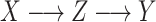is also a Markov chain, then these inequalities are strict. To show that is a monotone decreasing function of we establish a more general result (allowing each edge to have its own expected transition rate) and then examine the impact of increasing this expected rate on any given edge. A (probabilistic) coupling argument, together with an application of the DPI, leads to the claimed monotonicity. For the second part of Theorem 1 (concerning ), we consider the more informative (but unobservable) process in which one knows all the resampling events and the transitions within the tree (not just the states at the leaves). Let be the mutual information between and this more informative process. Using the DPI, we show that . A further application of the DPI to the more informative process shows that is a monotone increasing function of , and the claims about the values of and at = 0 and as then follow.

Statement and Sketch Proof of Theorem 2

Notice that the estimation error curves in the simulations (Fig. 2) appear to come down as increases. However, it is not at all clear whether they would continue to decrease towards zero or would instead converge to some nonzero value. We show that Yule trees with fixed heights allow for asymptotically precise estimation of both the root state and the relative rates as the number of leaves become large. To simplify the calculations, we increase the speciation rate (as this grows, the number of leaves is a random variable that tends to infinity). In Theorem 2, we allow more general models than the equal input model (as assumed in Theorem 1), encompassing most models used in phylogenetics, including the HKY model used in our simulations. We state Theorem 2 as follows (for details and full proof, refer to the Supplementary Appendix available on Dryad).

Theorem 2:

For any continuous-time evolutionary model with positive rate matrix , the ancestral root state, and the rate matrix (i.e., both the relative rates and the global rate ) can both be estimated with an error converging to zero on a Yule tree with fixed height, as the number of leaves tends to infinity. However, this is not possible for other tree shapes such as the star and Kingman coalescent trees.

A brief outline of the proof of Theorem 2 follows. To show that the root state can be accurately estimated with Yule trees, the primitive method of maximum parsimony (MP) (Maddison 1994; Felsenstein 2004) suffices (even though it is less accurate than ML). The proof that MP is consistent here combines two ideas: first we apply a (probabilistic) coupling argument which shows that it is enough to establish the result for an associated 2-state process; we then investigate this simpler process by deriving and analyzing a system of nonlinear differential equations (analogous to Gascuel and Steel, 2010).

To show that the entries in the rate matrix can also be consistently estimated with Yule trees, we consider an estimation method based on 3-leaf pendant subtrees. While such a method is not likely to be optimal (e.g., ML surely performs better) it is nevertheless sufficient to establish the theorem, and its simplicity allows for a tractable mathematical analysis that would be difficult for more complicated methods. We deal with 3-leaf pendant subtrees rather than just 2-leaf pendant subtrees (“cherries,” commonly used to estimate models from sequence data) for two reasons. First, it allows us to consider more general Markovian processes (in particular, we need not assume the Markovian process is time-reversible). Second, even for time-reversible models, an approach based on cherries only works if the leaves are very far from the root [so that the frequencies of states is at (or very close to) equilibrium]; in our setting, the tree has fixed height, and so generally the distribution of states amongst the leaves will not be very close to the equilibrium distribution (as observed in the simulations, a major difference with sequences where the equilibrium distribution is well approximated by the state frequencies among the sites, due to stationarity).

For each pair of not necessarily distinct states and we say that a 3-leaf pendant subtree is of type if leaf and one of the remaining leaves ( or ) have state and the other leaf (from the pair ) has state . We will also say that is of type if it is of type for some (including the case ), and that is typical if its height is no more than twice its expected height (in a Yule tree). For each pair of distinct states , let denote the number of typical 3-leaf pendant subtrees of type and denote the number of typical 3-leaf pendant subtrees of type .

Define to be twice the sum of the heights of the cherries of the typical 3-leaf pendant subtrees of type . Our proof uses the following simple estimator of the transition rates in the rate matrix : for any two (distinct) states , let . We show that is a statistically consistent estimator of as grows. The proof uses the distribution of the number and height (Rosenberg 2006; Stadler and Steel 2012) of 3-leaf subtrees in a Yule tree, together with further asymptotic arguments to show that converges in probability to .

For the second part of Theorem 2, first suppose that is a star tree. Then neither the ancestral root state, nor the equilibrium vector can be estimated accurately, even as . More precisely, the following nonidentifiability result holds. One can switch the root state to a different state, and adjust the parameters and to give an identical probability distribution on the data that such a tree generates regardless of how large is (details are provided in the Supplementary Appendix available on Dryad).

Next suppose that is a tree generated by the Kingman coalescent. For any value of , the state at the root of has an error that does not decrease to zero as . The proof relies on a well-known property (Wakeley 2009) of the coalescent tree : the shorter of the two edges incident with the root of has an exponential distribution with a mean that is asymptotic (as ) to , where is the height of the tree. A simple coupling argument (Mossel and Steel 2005) then shows that with probability at least (where is independent of but dependent on and the rate matrix ) the states at the leaves are independent of the root state of , and so the error in inferring the root state does not tend to zero as grows.

Simulation Protocol

To explore the behaviour of evolutionary models that are more complex and realistic than F81 and the equal input models used in Theorem 1, we performed computer simulations using the HKY model (Hasegawa et al. 1985; Felsenstein 2004). We generated Yule and coalescent trees with a number of tips equal to 100 and 1000. These trees were rescaled to have a total height of 1.0 (this is similar but not identical to the set-up for the mathematical proof of Theorem 2, where we fix the height of Yule trees, and vary the speciation rate to increase the expected number of leaves). Then, we simulated the evolution of a 4-state character according HKY with (transition/ transversion ratio) equal to 4.0, and equilibrium frequencies equal to 0.15, 0.35, 0.35, and 0.15, for A, C, G, and T, respectively. The HKY rate matrix was normalized as usual (i.e., the expected number of changes along a branch of length 1.0 was set to 1.0) and then multiplied by the global rate with values equal to 1/16, 1/8, 1/4, 1/2, 1, 2, 4, 8, and 16. For each of the tree models (Yule, coalescent) and values, 1000 trees and data sets were generated with = 100, and 500 with = 1000 for computing time reasons. For each data set we jointly estimated using the ML principle the and parameters, the four equilibrium frequencies, and the ancestral character state at the tree root. The latter was inferred using the MAP (maximum a posteriori) principle (i.e., the predicted state corresponded to the maximum of the posteriors among the four states), which is known to be optimal (Guiasu 1977). The estimation procedure was performed in three steps:

1. As the HKY parameters were unknown, we first used the Jukes and Cantor (JC) model (Felsenstein 2004) to obtain a rough estimate of by ML. Then, the tree was rescaled by multiplying all branch lengths by .

2. The resulting rescaled tree was given to PhyML (Guindon et al. 2010) along with the tips values, to estimate the and parameters (corresponding to KappaML and FreqML curves in Fig. 2). It has been demonstrated in a number of studies (e.g., Le and Gascuel, 2008) that the estimation of evolutionary model parameters remains accurate with approximate trees, as we have here regarding the branch lengths that are rescaled using (instead of which is unknown).

3. These ML-estimates of and were used to jointly infer the root state (RootMLfull in Fig. 2) and obtain a better ML-estimate of assuming an HKY model (GlobalRateML in Fig. 2). To quantify the loss of accuracy induced by the approximate estimation of the model parameters (, and ), we also estimated the root state with the model parameter values used to generate the data (RootMLtrue in Fig. 2).

A difficulty with ML-based estimations of , is that when the mutation rate is low, the root and tip states tend to be identical, and then is estimated to be zero. Similarly, with high rate is often estimated to be infinite. In both cases the estimation of the other parameters and root state becomes impossible (at least using a standard ML implementation, as PhyML). Thus, we imposed the constraint: , where is the true value and the estimate. This constraint was used with both JC-based (Step 1) and HKY-based (Step 3) estimations of .

To quantify the estimation error, for the numerical estimates (, and ) we measured the average over all data sets of the relative absolute error (e.g., with ), and the error of the four frequencies was further averaged over the four states. For the root state, we simply measured the frequency of the prediction errors. For comparison with the more accurate ML approach, a rough estimate of the equilibrium frequencies was also obtained by counting the number of state occurrences at the tree tips (FreqTips in Fig. 2). The error of this quick estimator (used in many ML software programs, but with sequences, not a single character) is clearly higher than FreqML, corresponding to the fact that with low and moderate the tip state frequencies do not reach the equilibrium probabilities (while they do with aligned genetic sequence data, as the root states of the multiple sites are (assumed to be) drawn based on the model equilibrium frequencies). We also compared the estimations of the frequencies and root state, with those obtained with a multinomial with trials drawn using the same nucleotide probabilities as in tree-based simulations. This multinomial model is equivalent to the tree model when is very large and/or the pending branches are extremely long. In this condition, the tips state values do not bring any information on the root state (), while the information on () is as high as possible with tips/trials (see Theorem 1). The root prediction error (RootMultin in Fig. 2) is then nearly equal to 0.65 (MAP returns C and G states with 0.5 probability each, and both have a prediction error of 0.65). The frequency estimation error was computed by simulations (FreqMultin in Fig. 2, 0.148 and 0.047 with = 100 and 1000, respectively). As expected, RootMultin RootML 0.65 with , and FreqMultin FreqML FreqTips with = 16 and Yule trees. Coalescent trees have much shorter pending branches, and the convergence of FreqML and FreqTips toward FreqMultin is slower.

All software programs (except PhyML) used to perform the simulation study were implemented in Common Lisp and are available on request. We used the version 3.3.20170530 of PhyML available from https://github.com/stephaneguindon/phyml.

Supplementary material

Data available from the Dryad Digital Repository: https://dx.doi.org/10.5061/dryad.6p55sp3.

Funding

This work was supported by the INCEPTION project (PIA/ANR-16-CONV-0005, OG).

References

- Arenas M., Weber C., Liberles D.A., Bastolla U.. 2017. ProtASR: an evolutionary framework for ancestral protein reconstruction with selection on folding stability. Syst Biol. 66:1054–1064. [DOI] [PubMed] [Google Scholar]
- Beaulieu J., O’Meara, B., Donoghue M.. 2013. Identifying hidden rate changes in the evolution of a binary morphological character: the evolution of plant habit in campanulid angiosperms. Syst. Biol. 62:725–737. [DOI] [PubMed] [Google Scholar]
- Brown J. 1994. Probabilities of evolutionary trees. Syst. Biol. 43:78–91. [Google Scholar]
- Casanellas M., Steel M.. 2017. Phylogenetic mixtures and linear invariants for equal input models. J. Math. Biol. 74:1107–1138. [DOI] [PubMed] [Google Scholar]
- Cover T., Thomas J. A.. 1991. Elements of information theory. New York: Wiley. [Google Scholar]
- Dudas G., Carvalho L.M., Bedford T., Tatem A.J., Baele G., Faria N.R., Park D.J., Ladner J.T., Arias A., Asogun D., Bielejec F., Caddy S.L., Cotten M., D’Ambrozio J., Dellicour S., Di Caro A., Diclaro J.W., Duraffour S., Elmore M.J., Fakoli L.S., Faye O., Gilbert M.L., Gevao S.M., Gire S., Gladden-Young A., Gnirke A., Goba A., Grant D.S., Haagmans B.L., Hiscox J.A., Jah U., Kugelman J.R., Liu D., Lu J., Malboeuf C.M., Mate S., Matthews D.A., Matranga C.B., Meredith L.W., Qu J., Quick J., Pas S.D., Phan M.V.T., Pollakis G., Reusken C.B., Sanchez-Lockhart M., Schaffner S.F., Schieffelin J.S., Sealfon R.S., Simon-Loriere E., Smits S.L., Stoecker K., Thorne L., Tobin E.A., Vandi M.A., Watson S.J., West K., Whitmer S., Wiley M.R., Winnicki S.M., Wohl S., Wölfel R., Yozwiak N.L., Andersen K.G., Blyden S.O., Bolay F., Carroll M.W., Dahn B., Diallo B., Formenty P., Fraser C., Gao G.F., Garry R.F., Goodfellow I., Günther S., Happi C.T., Holmes E.C., Kargbo B., Keïta S., Kellam P., Koopmans M.P.G., Kuhn J.H., Loman N.J., Magassouba N., Naidoo D., Nichol S.T., Nyenswah T., Palacios G., Pybus O.G., Sabeti P.C., Sall A., Ströher U., Wurie I., Suchard M.A., Lemey P., Rambaut A.. 2017. Virus genomes reveal factors that spread and sustained the Ebola epidemic. Nature 544:309–315. [DOI] [PMC free article] [PubMed] [Google Scholar]
- Edwards C.J., Suchard M.A., Lemey P., Welch J.J., Barnes I., Fulton T.L., Barnett R., O’Connell T.C., Coxon P., Monaghan N., Valdiosera C.E., Lorenzen E.D., Willerslev E., Baryshnikov G.F., Rambaut A., Thomas M.G., Bradley D.G., Shapiro B.. 2011. Ancient hybridization and an Irish origin for the modern polar bear matriline. Curr. Biol. 21:1251–1258. [DOI] [PMC free article] [PubMed] [Google Scholar]
- Evans W., Kenyon C., Peres Y., Schulman L.. 2000. Broadcasting on trees and the Ising model. Ann. Appl. Probab. 10:410–433. [Google Scholar]
- Felsenstein J. 2004. Inferring phylogenies. Sunderland, MA: Sinauer. [Google Scholar]
- Gascuel O., Steel M.. 2010. Inferring ancestral sequences in taxon-rich phylogenies. Math. Biosci. 227:125–135. [DOI] [PubMed] [Google Scholar]
- Gascuel O., Steel M.. 2014. Predicting the ancestral character changes in a tree is typically easier than predicting the root state. Syst. Biol. 63:421–435. [DOI] [PubMed] [Google Scholar]
- Grass Phylogeny Working Group II. 2012. New grass phylogeny resolves deep evolutionary relationships and discovers C4 origins. New Phytol. 193:304–312. [DOI] [PubMed] [Google Scholar]
- Guiasu S. 1977. Information theory with applications. New York: McGraw-Hill. [Google Scholar]
- Guindon S., Dufayard J.-F., Lefort V., Anisimova M., Hordijk W., Gascuel O.. 2010. New algorithms and methods to estimate maximum-likelihood phylogenies: assessing the performance of PhyML 3.0. Syst. Biol. 59:307–321. [DOI] [PubMed] [Google Scholar]
- Harding E. 1971. The probabilities of rooted-tree shapes generated by random bifurcation. Adv. Appl. Probab. 3:44–77. [Google Scholar]
- Hasegawa M., Kishino H., Yano T.. 1985. Dating of human-ape splitting by a molecular clock of mitochondrial DNA. J. Mol. Evol. 22:160–174. [DOI] [PubMed] [Google Scholar]
- Heintzman P.D., Froese D., Ives J.W., Soares A.E.R., Zazula G.D., Letts B., Andrews T.D., Driver J.C., Hall E., Hare P.G., Jass C.N., MacKay G., Southon J.R., Stiller M., Woywitka R., Suchard M.A., Shapiro B.. 2016. Bison phylogeography constrains dispersal and viability of the Ice Free Corridor in western Canada. Proc. Natl. Acad. Sci. USA 113:8057–8063. [DOI] [PMC free article] [PubMed] [Google Scholar]
- Heisenberg W. 1927. Uber den anschaulichen inhalt der quantentheoretischen kinematik und mechanik. Z. Phys. 43:172–198. [Google Scholar]
- Ishikawa S.A., Zhukova A., Iwasaki W., Gascuel O.. 2019. A fast likelihood method to reconstruct and visualize ancestral scenarios. Mol. Biol. Evol. (in press) 10.1093/molbev/msz131. [DOI] [PMC free article] [PubMed] [Google Scholar]
- Le S.Q., Gascuel O.. 2008. An improved general amino acid replacement matrix. Mol. Biol. Evol. 25:1307–1320. [DOI] [PubMed] [Google Scholar]
- Lemey P., Minin V.N., Bielejec F., Pond S., Suchard M.A.. 2012. A counting renaissance: combining stochastic mapping and empirical Bayes to quickly detect amino acid sites under positive selection. Bioinformatics 28:3248–3256. [DOI] [PMC free article] [PubMed] [Google Scholar]
- Lemey P., Rambaut A., Bedford T., Faria N., Bielejec F., Baele G., Russell C.A., Smith D.J., Pybus O.G., Brockmann D., Suchard M.A.. 2014. Unifying viral genetics and human transportation data to predict the global transmission dynamics of human influenza H3N2. PLoS Pathog. 10:e1003932. [DOI] [PMC free article] [PubMed] [Google Scholar]
- Lemey P., Rambaut A., Drummond A., Suchard M.. 2009. Bayesian phylogeography finds its roots. PLoS Comput. Biol. 5:e1000520. [DOI] [PMC free article] [PubMed] [Google Scholar]
- Liberles D. 2007. Ancestral sequence reconstruction. Oxford: Oxford University Press. [Google Scholar]
- Maddison D.R. 1994. Phylogenetic methods for inferring the evolutionary history and processes of change in discretely valued characters. Ann. Rev. Entomol 39:267–292. [Google Scholar]
- Marazzi B., Ané C., Simon M.F., Delgado-Salinas A., Luckow M., Sanderson M.J.. 2012. Locating evolutionary precursors on a phylogenetic tree. Evolution 66:3918–3930. [DOI] [PubMed] [Google Scholar]
- Matsumoto T., Akashi H., Yang Z.. 2015. Evaluation of ancestral sequence reconstruction methods to infer nonstationary patterns of nucleotide substitution. Genetics 200:873–890. [DOI] [PMC free article] [PubMed] [Google Scholar]
- Mossel E., Peres Y.. 2003. Information flow on trees. Ann. Appl. Probab. 13:817–844. [Google Scholar]
- Mossel E., Steel M.. 2005. How much can evolved characters tell us about the tree that generated them? In: Gascuel O., editor. Mathematics of evolution and phylogeny. Oxford: Oxford University Press; p. 384–412. [Google Scholar]
- Rosenberg N.A. 2006. The mean and variance of the numbers of r-pronged nodes and r-caterpillars in Yule-generated genealogical trees. Ann. Combin. 10:129–146. [Google Scholar]
- Semple C. and Steel M.. 2003. Phylogenetics. Oxford: Oxford University Press. [Google Scholar]
- Stadler T., Lambert A.. 2013. Birth-death models and coalescent point processes: the shape and probability of reconstructed phylogenies. Theor. Popul. Biol. 90:113–128. [DOI] [PubMed] [Google Scholar]
- Stadler T., Steel M.. 2012. Distribution of branch lengths and phylogenetic diversity under homogeneous speciation models. J. Theor. Biol. 297:33–40. [DOI] [PubMed] [Google Scholar]
- Wakeley J. 2009. Coalescent theory: an introduction. Greenwood Village: Roberts & Company Publishers. [Google Scholar]
- Werner G., Cornwell W., Sprent J., Kattge J., Kiers E.. 2014. A single evolutionary innovation drives the deep evolution of symbiotic N2-fixation in angiosperms. Nat. Commun. 5:4087. [DOI] [PMC free article] [PubMed] [Google Scholar]
- Yang Z. 2007. PAML 4: phylogenetic analysis by maximum likelihood. Mol. Biol. Evol. 24:1586–1591. [DOI] [PubMed] [Google Scholar]
- Yule G. 1925. A mathematical theory of evolution: Based on the conclusions of Dr. J. C. Willis, F.R.S. Philos. Trans. R. Soc. Lond. B 213:21–87. [Google Scholar]