Cherenkov‐excited luminescence scanned imaging using scanned beam differencing and iterative deconvolution in dynamic plan radiation delivery in a human breast phantom geometry

Abstract

Purpose

The purpose of this study was to demonstrate high resolution optical luminescence sensing, referred to as Cherenkov excited luminescence scanning imaging (CELSI), could be achieved during a standard dynamic treatment plan for a whole breast radiotherapy geometry.

Methods

The treatment plan beams induce Cherenkov light within tissue, and this excitation projects through the beam trajectory across the medium, inducing luminescence where there can be molecular reporter. Broad beams generally produce higher signal but low spatial resolution, yet for dynamic plans the scanning of the multileaf collimator allows for a beam‐narrowing strategy by recursively temporal differencing each of the Cherenkov images and associated luminescence images. Then reconstruction from each of these size‐reduced beamlets defined by the differenced Cherenkov images provides a well‐conditioned matrix inversion, where the spatial frequencies are limited by the higher signal‐to‐noise ratio beamlets. A built‐in stepwise convergence relies on stepwise beam size reduction, which is associated with a widening of the bandwidth of Cherenkov spatial frequency and resultant increase in spatial resolution. For the phantom experiments, europium nanoparticles were used as luminescent probes and embedded at depths ranging from 3 to 8 mm. An intensity modulated radiotherapy (IMRT) plan was used to test this.

Results

The Cherenkov images spatially guided where the luminescence was measured from, providing high lateral resolution, and iterative reconstruction convergence showed that optimization of the initial and stopping beamlet widths could be achieved with 15 and 4.5 mm, respectively, using a luminescence imaging frame rate of 5/s. With the IMRT breast plan, the original lateral resolution was improved 2X, that is, 0.08–0.24 mm for target depths of 3–8 mm. In comparison, a dynamic wedge (DW) plan showed an inferior image fidelity, with relative contrast recovery decreasing from 0.86 to 0.79. The methodology was applied to a three‐dimensional dataset to reconstruct Cherenkov excited luminescence intensity distributions showing volumetric recovery of a 0.5 mm diameter object composed of 0.5 μM luminescent microbeads.

Conclusions

High resolution CELSI was achieved with a clinical breast external beam radiotherapy (EBRT) plan. It is anticipated that this method can allow visualization and localization for luminescence/fluorescence tagged vasculature, lymph nodes, or superficial tagged regions with most dynamic treatment plans.

1. Introduction

The Cherenkov emission spectrum from MV radiation is composed of optical photons with a limited penetration in human tissue, and so irradiated tissue can be selectively excited with this light signal, which comes from the secondary electrons in the irradiated volume. Imaging the emitted light from the surface of tissue shows the entrance beam as projected on the patient's skin, which has motivated the concept of real‐time visualization of surface dose on patients during delivery of their external beam radiation therapy (EBRT).^{1, 2, 3} However, there is also potential to use Cherenkov light for molecular sensing of the tissue to assist in adaptive radiotherapy based upon the tumor microenvironment, using diagnostically useful molecular sensors (e.g., tissue oxygen pO2, acidity pH, or protein labels and reporters) within critical planning target volume (PTV) structures. The Cherenkov excited luminescence scanned imaging (CELSI) technique has been examined to sense luminescent molecular probes deep within tissue, using x‐rays generated by a therapeutic MV linear accelerator (LINAC), as shown in Fig. 1(a).^{4, 5} The outgoing Cherenkov and luminescence signals can be captured sequentially by a time‐resolved camera with different pulse delays relative to the LINAC radiation pulse. Typically LINAC pulses are 3–5 μs during which Cherenkov emissions can be detected, and time‐gating beyond this can be achieved for detection of luminescence with emission lifetimes near tens of μs. These signals can come from up to a few centimeters deep within the tissue if emitted in the near infrared wavelength range.

Figure 1.

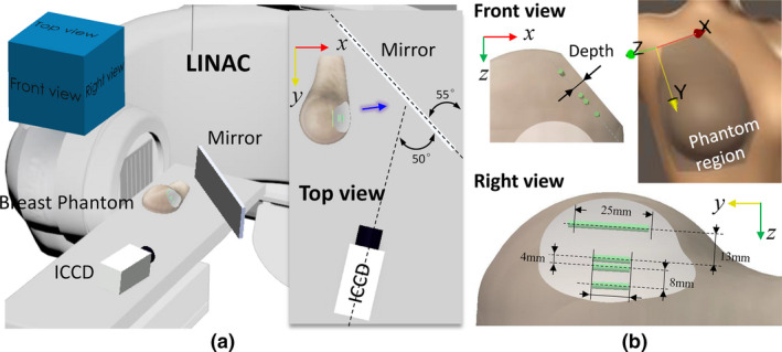
The experimental setup: (a) measurement geometry with a schematic inserted to specify the relative positions of the phantom, plane mirror, and camera, and (b) configuration of a full‐size breast phantom with four capillaries inside filled with europium (green cylinder). The blue arrow indicates the direction of detected luminescence light. [Color figure can be viewed at wileyonlinelibrary.com]

The major limiting factor in CELSI is the signal attenuation from optical light blur going from the point of luminescence emission to the tissue surface, but this can be compensated for by knowledge of where the excitation x‐ray scan beam is incident within the tissue. There is also a smaller contribution from the Cherenkov light blur as well. The optical signal is attenuated and blurred out by elastic scattering and small absorption effects as the photons pass through the tissue, which is largely modeled as a diffusive process in thick tissue. The degradation model can be expressed as a convolution equation:

$$\mathbf{Y}=\mathbf{X}\otimes {\mathbf{P}}_{\mathrm{Chk}}\otimes {\mathbf{P}}_{\mathrm{lum}}+\mathbf{N}$$ (1)

where Y is raw luminescence; P _Chk and P _lum denote the position‐dependent point spread functions (PSF) of Cherenkov and luminescence, respectively; X is the undistorted latent luminescence image; ⊗ is the convolution operator; and N is acquisition noise, which can be significant. It is assumed here that the system is time invariant, and linear. For general applications of CELSI, the contribution to Cherenkov blur from the x‐ray and electron scattering is important to include for completeness, complicating the estimation of P _Chk, as it requires full Monte Carlo radiation modeling for this to be accurate. In comparison, P _lum could often be reasonably accurately estimated with elastic photon transport models such as diffusion theory or optical elastic scattering Monte Carlo which are less computationally intensive.⁶ With the analysis above, the deconvolution operation in Eq. (1) is ill‐conditioned, and so is mitigated through the use of regularization techniques, that is, replacing the ill‐conditioned problem with a well‐conditioned one.⁷

In this paper, a novel iterative deconvolution method is proposed for CELSI with an edge‐scanned excitation beam. Since smaller beam sizes have been demonstrated to produce higher spatial resolution for CELSI,⁸ in this method, raw Cherenkov measurements were iteratively differenced to form width‐reduced effective excitations (termed as beamlets), improving the sensitivity to high spatial frequency data. The resultant stepwise widened frequency band renders a potential way for a converged iteration process towards a realistic result with broadband frequency. In the first iteration, difference Cherenkov measurement with a largest scanning position gap (b) was used to deconvolve corresponding difference luminescence one. This relationship between the cropped excitation and its resultant emission is based on the superposition principle of linear system. Then the calculated result was in turn utilized as a “noise‐reduced measurement” to be deconvolved for next iteration. The reconstruction methodology was tested out with a beam geometry and radiation dose used in a typical fraction of intensity modulated radiation therapy (IMRT)⁹ to assess the type of information that could be derived in standard fractionated breast radiotherapy. Experiments were performed with a progressive series of test phantoms, which illustrated the capabilities for depth recovery and high spatial resolution, and luminescent agent, which has the potential for protein reporter imaging.

2. Materilas and methods

2.A. System and setup

Most EBRT treatment plans in patients dynamically shape the beam with the multi‐leaf collimators (MLCs) and jaws within the LINAC, targeting the tumor region and minimizing dose to nearby critical structures. As a result, it was hypothesized that the natural spatial modulation done in clinical radiotherapy could be used to achieve an enhanced CELSI, based upon how the beamlets were formed. To investigate this, we herein examined a widely used IMRT treatment plan. A clinical radiotherapy accelerator (Varian Clinac 2100 CD, Varian Medical Systems, Palo Alto, CA, USA) was used to perform the breast IMRT with the following parameters: photon energy of 6 MV, radiation dose of 210 MU, dose rate of 600 monitor units per minute (MU/min), a fixed repetition rate of 360 Hz with a pulse width of 3.25 μs, and gantry angles of 270° and 90° used for medial and lateral tangent beamlets, respectively. For proof‐of‐concept, measurements were collected only for the geometry with 270° gantry position in this paper. The luminescence was imaged by a gated, intensified charge‐coupled device (ICCD, PI‐MAX4 1024i, Princeton Instruments, Acton, MA, USA). The camera worked with a focal length of 85 mm and f/1.2 lens. The luminescence signal was detected with time‐gated acquisition of the ICCD (100 μs integration time and 4.26 μs delay after each x‐ray pulse). The luminescence images were acquired with 100× gain on the ICCD intensifier, 30 pulses integrated on‐chip as accumulations prior to each frame readout, and 2 × 2 hardware pixel binning at readout, from chip size of 1024 pixels × 1024 pixels.⁵ Cherenkov images were acquired in the same way, but with 0 μs pulse delay and a 3.5 μs integration time.⁵

The transmittance measurement geometry is shown in Fig. 1(a), where a plane mirror was used to reflect the outgoing Cherenkov and luminescence into a horizontally positioned camera as indicated in the insert. Note that only the reflected luminescence portion was captured by the camera. A tilt camera was intent to keep it within the bench area. A full‐size right breast phantom was made of soft clay (B00LH2DWDW, Sculpey Inc., Stockbridge, GA) to facilitate targets embedding, and demonstrated with a spatial frequency domain imaging (SFDI) system (Reflect RS, Modulated Imaging Inc., Irvine, CA) to have tissue optical properties of ${\mu }_a=0.008$ and ${\mu }_s^{\prime }=2$ mm⁻¹ at 625 nm.¹⁰ The phantom was computed tomography (CT)‐scanned and the shape transferred to the Eclipse treatment planning system (Varian Medical Systems, Palo Alto, CA) for radiotherapy treatment planning. The luminescent probe used europium nanoparticles, which, characterized by long lifetime, sharp spectral profiles, nontoxic to cells, etc., have been widely used to tag proteins with antibody labeling.^{11, 12} As indicated in Fig. 1 (b), four europium capillaries (0.5 μM) with a diameter of 0.5 mm were placed at a depth of 5 mm to mimic blood vessels. There was no specific reason for tilting the capillaries with respect to the Y‐Z coordinate system, that was just the configuration of the breast phantom. To keep the same depths for the capillaries, a part of the phantom lateral surface was cropped to be flat as shown in the right view and the IMRT treatment plan was made before cropping.

2.B. Theory

A fast and simple method to solve this task posed in Eq. (1) is Wiener filtering¹³ which is essentially a regularized inversion of the convolution via the Fourier domain. However, this direct or linear method is prone to noise amplification at high frequencies and ringing artifacts especially when P _lum is noninvertible.¹⁴ Many algorithms have been proposed to solve this problem: a regularized constraint based upon total‐variation minimization was introduced to stabilize the solution^{15, 16}; in a wavelet basis approach, the true image can be efficiently represented by a few large coefficients while noise distributes over a large number of smaller ones, so that either thresholding or filtering strategy could be leveraged to denoise the deconvolved result.^{17, 18} Although direct deconvolution is computationally expensive, most solutions are based on iterative or nonlinear strategies. The advantages of iterative deconvolution include¹⁹: (a) a priori knowledge of the data's statistics are usually not required (sometimes called blind deconvolution); (b) prior information can easily be incorporated into the algorithm as a constraint term; and (c) iterations can cease when errors exceed a given bound. Most of these are based on Van Cittert's method, where a correction item times a real relaxation factor was added to adjust the iteratively obtained result at a given rate of convergence.²⁰ Others are mostly based on a Bayesian theorem with maximum likelihood (ML) solution, for example, Landweber⁷ and Lucy–Richardson deconvolutions^{21, 22} have been developed for Gaussian and Poisson noise types, respectively. Since the inverse process is ill‐conditioned, negative effects will emerge as the iteration number increases or the regularization decreases. This is especially obvious when the iteration number becomes infinitely large, and there is only noise left. For iterative deconvolution, extra attention should be paid to defining a stopping criterion and acceptable rate of convergence. Most convergence criteria in iterative deconvolution are based on mathematical approaches with limited a priori information involved in measurement, e.g., inherent non‐negativity and continuity.^{23, 24, 25} The conclusion derived from the above analysis was that an effective deconvolution depends on the factors of PSF estimation, noise control, and convergence criterion for iterative approaches.

To get a decreased “beam size” for higher spatial resolution and acquisition‐noise suppression, we utilized difference Cherenkov images between two scanning positions with an overlapped scanning area, which resulted in corresponding difference luminescence images according to the superposition principle. An absolute form of the difference images in between the scanning positions of i and i + b can be expressed as

$$\mathrm{\Delta }{\mathbf{\Psi }}_{i,b}=|{\mathbf{\Psi }}_i-{\mathbf{\Psi }}_{i+b}|,\mathbf{\Psi }\in \{\mathbf{C},\mathbf{Y}\},$$ (2)

where C and Y are the raw measurement of Cherenkov and luminescence, respectively. It is noteworthy in the above equation that $i\le \mathrm{I}-b$ with I being the maximum scan number. As an example, the resultant Cherenkov merged with roomlight images at scanning positions i = 20, 40 and 60, are shown in the first column of Fig. 2(a), and the associated difference images are shown in the second and third columns for b = 20 and 1, respectively. It can be seen from Fig. 2(b) that spatial resolutions improve in the progression from edge‐scanning to line‐scanning, as expected. However, much more noise can be found for the case of b = 1, because of the strong positive dependency of signal‐to‐noise ratio (SNR) on the x‐ray beam size in CELSI.⁸ Consequently, we started the iterative deconvolution procedure from a large beamlet size. Considering $\mathrm{\Delta }{\mathbf{C}}_{i,b(-20)}$ covers only a small range of effective spatial frequency (those with a magnitude below 10% could be noise), as shown in the leftmost image of Fig. 3, deconvolution of Eq. (1) is cutoff at a limited spatial frequency ω = R, termed the cutoff frequency. The small cutoff frequency R and difference operation in Eq. (2) make acquisition noise N small enough, which made the deconvolution of Eq. (1) well‐conditioned. The deconvolution approach used here is as follows

$$\mathrm{\Delta }{\mathbf{X}}_{i,b}^{\prime }=\left\{\begin{array}{cc}{F}^{-1}〈\frac{F⟨\mathrm{\Delta }{\mathbf{Y}}_{\mathit{i},\mathit{b}}⟩(\omega )}{F⟨\mathrm{\Delta }{\mathbf{C}}_{\mathit{i},\mathit{b}}⟩(\omega )+\epsilon }〉,\hfill & if|\omega |<R\hfill \\ 0,\hfill & if|\omega |\ge R\hfill \end{array}\right.,$$ (3)

where ${\mathbf{X}}^{\prime }=\mathbf{X}\otimes {\mathbf{P}}_{\mathrm{lum}}$; ԑ is an infinitesimal integer to circumvent division by zero; and $F$ and $F^{-1}$ represent Fourier and inverse Fourier transforms, respectively.

Figure 2.

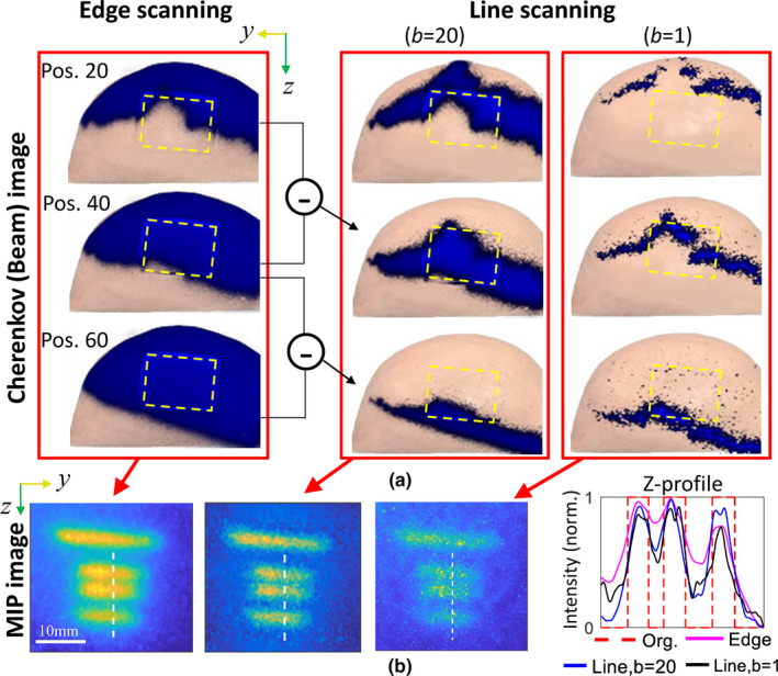
Comparisons among the results recovered from different beamlet size: (a) Cherenkov images of the original and difference beamlets projected on the breast phantom, and (b) the maximum intensity projection images and corresponding Z‐profiles along the white dashed lines. The yellow frames in (a) indicate the regions of interest. Each of the Z‐profiles in (b) was normalized to the maximum intensity. [Color figure can be viewed at wileyonlinelibrary.com]

Figure 3.

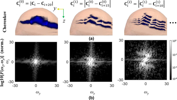
The spatial frequency images for recursive difference irradiation beamlets from the intensity modulated radiotherapy scan, with position gaps being 20, 15, and 10 from left to right columns: (a) the corresponding difference Cherenkov images in the top row, and (b) two‐dimensional spectrogram images in the bottom row. (a) denotes the Cherenkov intensity map captured at the ith scanning. [Color figure can be viewed at wileyonlinelibrary.com]

As a potential way to improve lateral resolution, we could further reduce the beamlet size by continuing recursive difference operations on the baseline result $\mathrm{\Delta }{\mathbf{C}}_{i,b^{(0)}}^{(0)}$, and the kth expression is

$${\mathbf{C}}_i^{(k)}=\mathrm{\Delta }{\mathbf{C}}_{{i,b}^{k-1}}^{(k-1)},k>0.$$ (4)

As seen from Fig. 3, a widening of the spatial frequency bandwidth can be found for recursive difference Cherenkov images, enriching the resultant luminescence images with broadband frequency, and implying a potential convergence of the iterative procedure.²⁶ A crucial step in this method is to use the deconvolved result from last iteration as the “measured” image for present deconvolution:

$${\mathbf{Y}}_i^{(k)}=\mathrm{\Delta }{\mathbf{X}}_{{i,b}^{(k-1)}}^{\prime (k-1)},$$ (5)

due to the much lower SNR of the raw difference “measured” luminescence images as discussed for Fig. 2(b). For the kth iteration, an iterative deconvolution can be formed as:

$$\mathrm{\Delta }{\mathbf{X}}_{i,b^{(k)}}^{\prime (k)}=\left\{\begin{array}{cc}{F}^{-1}〈\frac{F〈\mathrm{\Delta }{\mathbf{Y}}_{i,b^{(k)}}^{(k)}〉(\omega )}{F〈\mathrm{\Delta }{\mathbf{C}}_{i,b^{(k)}}^{(k)}〉(\omega )+\epsilon }〉,\hfill & if|\omega |<R^{(k)}\hfill \\ 0,\hfill & if|\omega |\ge R^{(k)}\hfill \end{array}\right.,$$ (6)

where $R^{(k)}$ was inversely proportional to the beamlet size as discussed, and its specific value could be chosen according to effective frequency coverage as exampled in Fig. 3. The recovered image ${\mathbf{X}}_i^{(k)}$at each iteration is a maximum intensity projection (MIP) of $\mathrm{\Delta }{\mathbf{X}}_{i,b^{(k)}}^{\prime (k)}(=\mathrm{\Delta }{\mathbf{X}}_{i,b^{(k)}}^{\prime (k)}\otimes {\mathbf{P}}_{\mathrm{lum}}$) for all scanning positions. As mentioned earlier, the SNR can reach a noise floor level as the beamlet size decreases. Further investigation of stopping criterion of the iteration process is presented in Section 3.A. After the iterative deconvolutions, the latent image, X, can be obtained by continuing to complete a direct deconvolution with P _lum, which was calculated from the diffusion equation combined with a Robin‐type boundary condition.²⁷

3. Results

3.A. Investigations of iteration criterion

In Fig. 4(b), we show results obtained via three different iterative‐deconvolution strategies (denoted in the Figure as #1, #2 and #3), each of which is defined by initial choice of b and an associated sequence of iterations of Eq. 6 (as shown in labels above the images). The corresponding z‐profiles are summarized in Fig. 4(b), with each plot displaying curves for different iteration strategy. To quantify the spatial resolution performance, a metric of success was introduced, defined as $r=\left({\mathrm{I}}_{\max }-{\mathrm{I}}_{z=69\mathrm{mm}}\right)/\left({\mathrm{I}}_{\max }-{\mathrm{I}}_{\min }\right)$, with I_max and I_min being the maximum and the minimum in the z‐profile, essentially providing a relative measure of contrast recovery. Note that the r value was only calculated for the two most closely spaced capillaries, the distance of which along the white dashed lines is centered at z = 69 mm as indicated in Fig. 4(b). With this definition, r = 1 represents that the two targets can be completely separated, with full contrast recovery. In the characteristics of the human vision system, it is normally assumed that two targets are distinguishable for r > 0.1 (when a 10% dip in intensity is observed between them).²⁸

Figure 4.

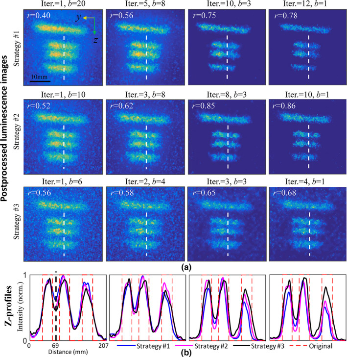
Comparisons among the proposed method with different iteration strategies indicated with #1(top), #2(middle), and #3(bottom), respectively: (a) the resultant luminescence images, and (b) corresponding z‐profiles along white dashed lines in (a). r values are inset in each image to qualify contrast recovery. Each of the z‐profiles in (b) was normalized to the maximum intensity. (A full scanning video of iteratively tailored Cherenkov image sequences and the resultant luminescence sequences for iteration strategy #2 is available in Video S1.) [Color figure can be viewed at wileyonlinelibrary.com]

We investigated the effect on r of varying initial beamlet size b and number of iterations, choosing initial values 20, 10, and 6 for b. As shown in Fig. 4(a), for any choice of initial b, r increases significantly with number of iterations until b = 3. Consequently, b = 3 was taken as a beamlet size for the final iteration in this context, corresponding to an actual beamlet width of 3 mm. A convergence condition could be based on the change of r, that is, the iteration process stops in case of a small change of r. Considering that each iteration is associated with a decreased beamlet size, we would expect that convergence is reached with fewer iterations by beginning with a narrower line beam (i.e., smaller b). As shown in the different rows of Fig. 4(a), those with initial beamlet sizes of b = 20 and b = 10 show similar performance for the final iteration. In comparison, the one starting from b = 6 led to a final image with more noise, although a slightly higher r value was found for the first iteration. This implies that, the amplitude of measurement noise ranged within this frequency passband was considerable, leading to an unstable deconvolution. In conclusion, an optimized iteration scheme could start from b = 10 and end at b = 3, which was used for all the deconvolutions below in case of no specific statement. With a readout frame rate of 5 fps from the camera and a dose rate of 600 MU/min used in the IMRT plan, b values of 10 and 3 correspond to physical metrics of 15 and 4.5 mm, respectively. These values might be different for other treatment plans with distinct dose rate and scanning area, depending on the movement speed of the leaves or jaws.

3.B. Imaging for varying target depths

In this section, the effect of increasing target depth was analyzed. The raw MIP images and processed results are shown in the top and middle rows of Fig. 5, respectively, and the corresponding Z‐profiles are shown in the bottom row. We can see that the iteratively deconvolved results show great improvement compared to the original images. With increasing target depth, separate capillaries become less readily distinguishable. In particular, for the deepest targets embedded at 8 mm, the middle two capillaries with a gap of 4 mm are characterized with an r of 0.27. After iterative deconvolution, the background becomes clear and contrast recovery is enhanced to r = 0.74. Note that the excitation PSF estimated by Cherenkov images were fixed for different target depths. For deeper targets, diffusive scattering of emission photons is more responsible for image blurring than is diffusive scattering of excitation photons.

Figure 5.

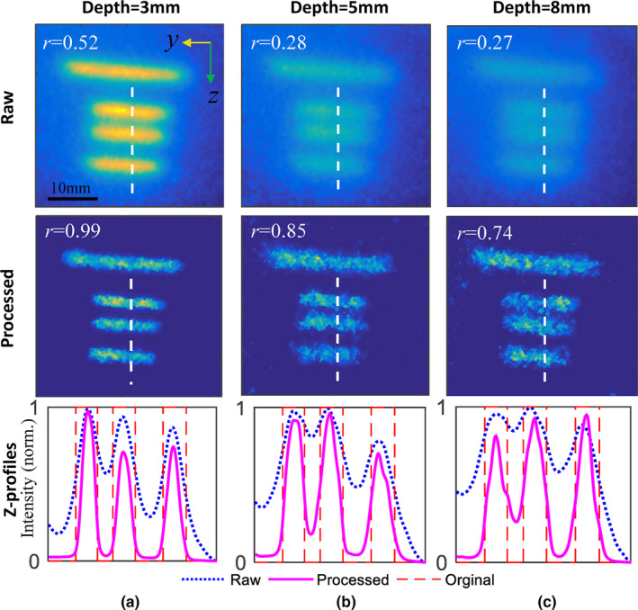
Raw (top) and postprocessed (middle) luminescence images for target depths of (a) 3 mm, (b) 5 mm, and (c) 8 mm, respectively. The corresponding Z‐profiles were plotted in the bottom row along the dashed white lines in above images. Each Z‐profiles was normalized to the maximum intensity. [Color figure can be viewed at wileyonlinelibrary.com]

3.C. Modulation transfer function analyses

To quantify spatial frequencies that can be resolved vs depth, raw images, as shown in the upper row of Fig. 6, were analyzed to obtain modulation transfer functions (MTFs). Results as measured for target depths of 3, 5, and 8 mm are plotted in Figs. 6(a)–6(c), respectively, where deconvolved results truncated at iteration number of 1, 3, 6, and 8 are shown for reference. The line spread functions (LSFs) are inset correspondingly and fitted to Gaussian curves in the subplots, and demonstrate the available spatial frequencies from which information can be obtained. Spatial resolutions achievable are related to the inverse of the MTF function where there is measurable amplitude, and here it was taken as 10% of the maximum. These are defined at different target depths, as recorded in Table 1, where the effective lower limit on resolution was estimated. It can be seen from Table 1 that: (a) the spatial resolution increases greatly with iteration number for all target depths — the value as estimated for 8th iteration is almost double the value estimated for the first iteration; (b) resolution also improves with reduced depth for fixed iteration number, and the rate of improvement increases with number of iterations. For example, the rate of improvement between 5 and 8 mm increased from 9.7% in the 1st iteration to 26% in the 8th iteration. This can be attributed to the enhanced higher spatial frequency response with the increasing iterations due to the narrowed Cherenkov excitation source as analyzed in Fig. 3.

Figure 6.

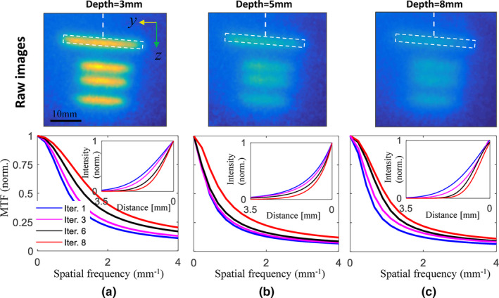
Normalized modulation transfer function curves estimated for target depths of (a) 3 mm, (b) 5 mm, and (c) 8 mm, respectively, and different number of iterations. The insert curves correspond to Gaussian‐fitted line spread functions along the white dashed lines indicated in the top row images. [Color figure can be viewed at wileyonlinelibrary.com]

Table 1.

Inverse of limiting spatial frequency (10% of the modulation transfer function amplitude) defined at varying depths for different number of iterations

Depth (mm)	Iter.
	1 (mm)	3 (mm)	6 (mm)	8 (mm)
3	0.23	0.16	0.10	0.08
5	0.41	0.35	0.25	0.19
8	0.45	0.35	0.28	0.24

3.D. Comparisons between CELSI with IMRT and DW treatment plans

As discussed before, an original edge‐scanning x‐ray or electron irradiation is requisite to accommodate difference operations to create downsized beamlets. Fortunately, most modern radiation treatment plans were designed in this way to minimize radiation exposure in normal tissue. Here, another plan named a dynamic wedge (DW) was investigated, which instead uses the jaws in the LINAC to slowly close to the desired shape. In this experiment, three europium capillaries (0.5 μM) with a diameter of 0.7 mm were placed at a depth near 5 mm in the breast phantom, as shown in Fig. 7(a), while the measurement geometry is the same as that used in Fig. 1. Cherenkov images in the third iteration with b = 8 are shown in Fig. 7(b) for both IMRT and DW plans. The radiation dose used was 204 MU, and other settings for the LINAC including beam energy, dose rate, geometry settings, and impulse duration were kept the same for the DW plan as those for the IMRT plan. The recovered images with this proposed method are shown in Fig. 7(c). It can be seen that the DW result presented degraded image fidelity with lower signal‐to‐background contrast recovery. This can be explained by the fact that, in comparison with the IMRT plan, much more radiation dose of the DW plan was delivered with a fixed beam shape, which means the difference operations would result in zero Cherenkov and luminescence for this part of dose.⁸ To investigate lateral spatial resolution, Z‐profiles along the white dashed lines in Fig. 7(c) are shown in Fig. 7(d), and we can see that imaging with IMRT obviously outperforms that with the DW plan. This is due to the expanded spatial frequency along multiple directions as shown in the two‐dimensional (2D) spectra of Fig. 7(b), which improved spatial resolution correspondingly.²⁵ In order to determine the difference in spatial frequency distribution, the beam mappings in Fig. 7(b) can be examined, where the edges of the IMRT beam are not as smooth as that in DW result. This was caused by the MLC mechanics in the former, where the leaf movement is not well synchronized.

Figure 7.

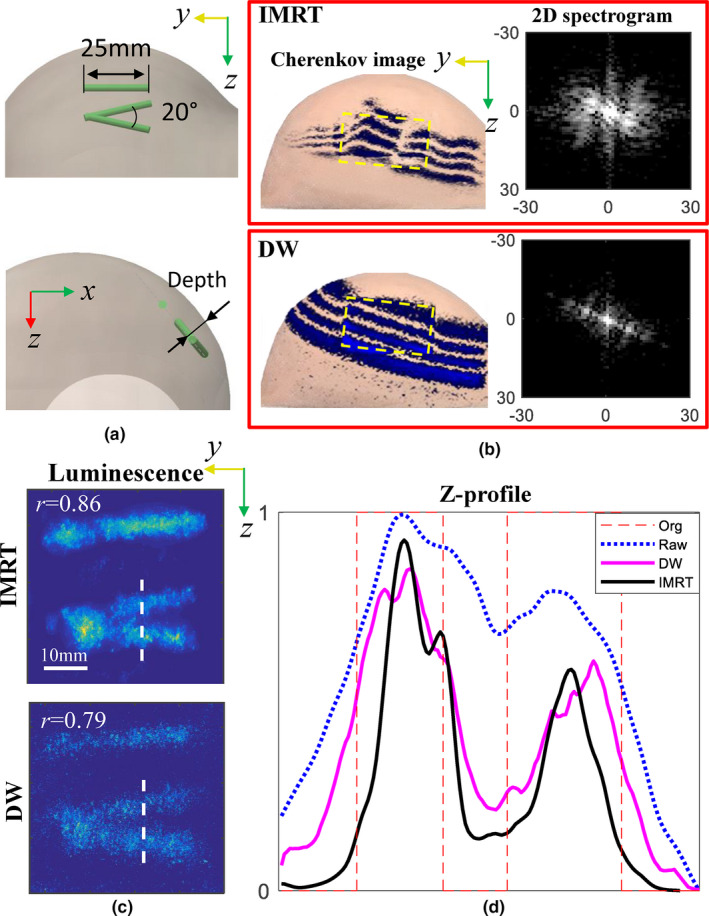
Comparisons of imaging results by using intensity modulated radiotherapy and dynamic wedge (DW) plans: (a) the phantom configuration, (b) Cherenkov and two‐dimensional spectrogram images, (c) luminescence images, and (d) the corresponding Z‐profiles across the dashed white lines in (c). The raw data in (d) were measured for the DW plan. [Color figure can be viewed at wileyonlinelibrary.com]

3.E. 3D CELSI Scan and Reconstruction

Three‐dimensional (3D) restoration has been realized for CELSI using a light sheet imaging approach.⁴ The measurement geometry is shown in Fig. 8(a), while the difference is that the camera was placed at the top of the phantom and light sheet was created by differencing the original edge‐scanned beam [Fig. 8(b)]. By shaping the x‐ray beam into a thin sheet and observing the Cherenkov‐excited luminescence orthogonally to the sheet beam, we were able to capture a luminescence image emanating from only a single plane within the phantom. In this section, we achieved 3D distributions for both Cherenkov and luminescence light. To demonstrate this, a 3 mm diameter and 8 mm length europium‐microsphere‐containing tube at a concentration of 0.5 μM was embedded in the breast phantom at a depth of 10 mm, as indicated in Fig. 8(a), to mimic a lymph node.

Figure 8.

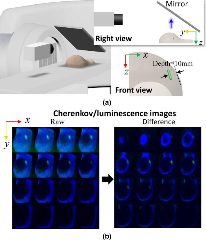
A three‐dimensional realization for Cherenkov and luminescence distributions with a dynamic wedge treatment plan: (a) the experimental setup with the linear accelerator lateral, phantom, and intensified charge‐coupled device camera on the patient bed, and (b) raw and differenced Cherenkov images. A right view to specify the relative positions of the phantom, mirror, and camera is inserted in (a), and below that is the front view to show the target location. The blue arrow indicates the direction of detected luminescence light. [Color figure can be viewed at wileyonlinelibrary.com]

Processing of the raw measurements is similar to that for the 2D imaging, including three steps: (a) iterative deconvolution for luminescence images frame‐by‐frame, (b) restorations for 3D Cherenkov and luminescence distributions, and (c) diffusion corrections for luminescence light. Operations in step 1 are similar as those for 2D imaging by using Eqs. (4)–(6). The luminescence MIP images before and after deconvolution are shown in Fig. 9(a), as well as x‐profiles along the white dashed lines. In step 2, to realize 3D restoration, we have to know z‐positions of all layer‐scanned beamlets. As a result, single‐line shaped beamlets as shown in the difference Cherenkov image of Fig. 8(b) were utilized to replace the above multiple‐line ones in Fig. 7(a). For this, only the positive pixels of the difference images were stored, and so Eq. (2) can be rewritten as

$$\mathrm{\Delta }{\mathrm{\Psi }}_{i,b}={\left({\mathrm{\Psi }}_i-{\mathrm{\Psi }}_{i+b}\right)}^{0^{+}},i+b\le \mathrm{I},$$ (7)

where the superscript 0+ means only the positive elements were preserved. In addition, for advanced radiation treatment, gantry rotation generally forces a back‐and‐forth movement of the leaves in the MLC to adjust the beamlet area dynamically. Consequently, a one‐way scanning episode was sufficient to sample and reconstruct a 3D image stack of the volume.

Figure 9.

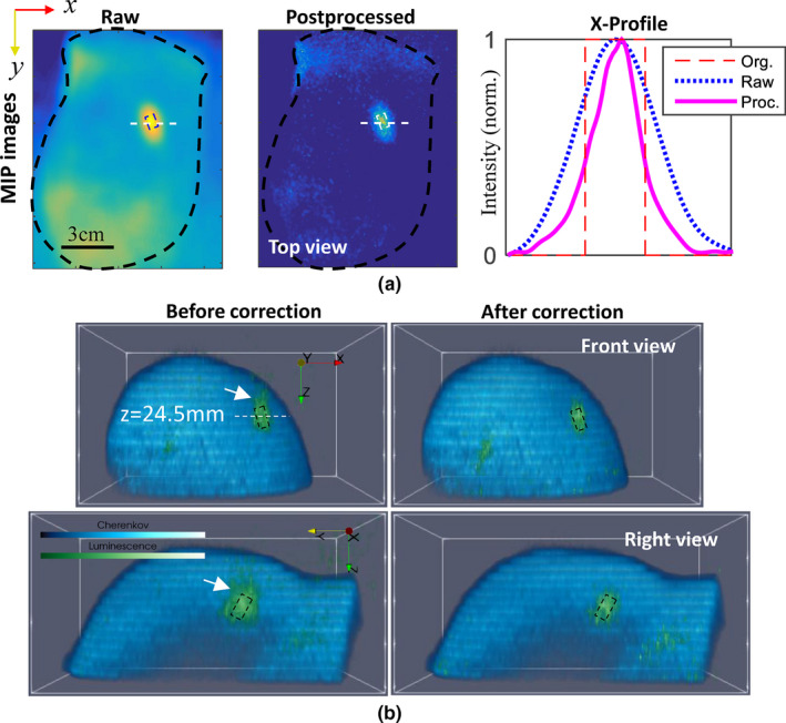
Postprocessed results: (a) Iteratively deconvolved luminescence maximum intensity projection image and corresponding X‐profiles along the dashed white lines, and (b) three‐dimensional (3D) recovery of Cherenkov and luminescence distributions. 3D luminescence distributions are shown without and with diffusion correction in the left and right rows of (b). Dashed frames indicate real positions, and white arrows in (b) point to the part outside of the frames before corrections. [Color figure can be viewed at wileyonlinelibrary.com]

A three‐dimensional view of the recovered Cherenkov light distribution is shown in Fig. 9(b), whose surface profile was extracted to acquire depth information. Then diffusion corrections can be made for luminescence target based on photon transport models, e.g., diffuse approximation for simplicity.⁴ To some extent, step 1 (iterative deconvolution) and step3 compensated for the diffusion effects along X‐Y plane and Z‐direction, respectively. In step 2, depth resolution basically depended on the frame‐rate of the camera. The final 3D combinations of Cherenkov and luminescence, before and after the corrections, are displayed in the left and right columns of Fig. 9 (b), respectively. As expected, after correction (a) the “skin effect” was mitigated, i.e., the centroid of the target moved from z = 22.9 mm to z = 24.2 mm, closer to its real position as indicated in the front‐view of Fig. 9(b); (b) the target volume shrunk toward its true size as indicated with black boxes in the front‐ and right‐ views of Fig. 9(b).

4. Discussion

CELSI has been previously demonstrated to have an imaging depth of 3–4 cm,^{4, 5, 29} which is ideal for imaging breast lymph nodes and superficial tumors. In supplement to this, this study focused on a method for high resolution CELSI recovery to image mesoscopic biological structures (e.g., subcutaneous blood capillaries and lymphatics) testing for Ø = 0.5 mm as used in the phantom experiments. Based upon our previous conclusion from studying patterned illumination, that is, that the SNR for induced luminescence is proportional to the target area covered within the irradiation beam,⁸ the advantage of IMRT or DW scanning come in with large areas providing large signals for detection. As discussed before, downsized beam could be achieved by an original edge‐scanned irradiation, and thus the edges should sweep over the target. This could be satisfied for most inverse‐planning based dynamic treatment plans, for example, IMRT, volumetric modulated arc therapy (VMAT),²⁹ and DW. However, this is not the case for the simple and older forward‐planning based ones, for example, 3D conformal radiation therapy (3DCRT), where the profile of each radiation beam for each gantry angle is shaped to fit the profile of the target from a beam eye view.³⁰ To uniformly cover the target, radiation is usually delivered from multiple LINAC gantry positions, and the trend is to be more conformal which means more beamlets from more angles, providing high spatial frequency scan information. In this way, 3D imaging combines very nicely with the trends in therapy, and provides a dataset quite analogous to x‐ray CT.

5. Conclusion

This paper described a resolution enhancement strategy to postprocess CELSI measurements obtained from standard breast radiation treatment plans. Instead of making a tradeoff between spatial resolution and signal SNR, the proposed method benefits from a well‐conditioned deconvolution and high spatial frequency resolved luminescence that results from wide and narrow beams, respectively. In order to address the ill‐conditioned deconvolution of narrow beams, a successive approximation approach was developed to recursively generate difference Cherenkov images and instead take the pre‐deconvolved result as a distorted luminescence measurement. A built‐in stepwise convergence relies on stepwise decreasing of the beam size, which is associated with a widening of the bandwidth of Cherenkov spatial frequency and resultant increasing spatial resolution.²⁵ In comparison to luminescence, the Cherenkov signal is much stronger and its fundamental spatial frequency is limited below a certain value (as shown in Fig. 3), which is set as a cutoff frequency for deconvolution to reduce its ill‐posed nature. The stopping criterion was made based upon how small of a beam size would be acceptable for measurement with reasonable SNR. Investigation of the iteration criterion in Section 3.A showed that an effective and conservative iteration could start from a beamlet width b = 10 and end by b = 3, corresponding to physical sizes of 15 and 4.5 mm, respectively. These values were tested for a medium with tissue‐like optical properties and a moderate target depth of 5 mm. An added benefit of this method is that the excitation PSF could be estimated based on the Cherenkov image locations, instead of relying upon the luminescence for localization. Although the measured P _Chk is not the exact width as Cherenkov deeper in the tissue, the deconvolution with P _Chk shapes is a reasonable approach for superficial applications through a few cm where the beamlet width does not change all that much.³

In basic applications of luminescence/fluorescence imaging, oxygen sensitivity lifetime probes have been used to directly sample partial pressure of oxygen (pO₂) in vivo for mammalian tissue with CELSI.^{4, 5, 31} We could readily apply the proposed method into these CELSI procedures and might improve the mapping of oxygen concentration in tissues.

Conflict of interest

The authors have no conflicts to disclose.

Supporting information

Video S1. Fully‐scanned Cherenkov and the resultant luminescence sequences.

References

- 1. Andreozzi JM, Zhang R, Gladstone DJ, et al. Cherenkov imaging method for rapid optimization of clinical treatment geometry in total skin electron beam therapy. Med Phys. 2016;43:993–1002. [DOI] [PMC free article] [PubMed] [Google Scholar]
- 2. Andreozzi JM, Brůža P, Tendler II, et al. Improving treatment geometries in total skin electron therapy: experimental investigation of linac angles and floor scatter dose contributions using Cherenkov imaging. Med Phys. 2018;45:2639–2646. [DOI] [PubMed] [Google Scholar]
- 3. Andreozzi JM., Mooney KE, Brůža P, et al. Remote Cherenkov imaging‐based quality assurance of a magnetic resonance image‐guided radiotherapy system. Med Phys. 45: 2647–2659. [DOI] [PubMed] [Google Scholar]
- 4. Brůža P, Lin H, Vinogradov SA, Jarvis LA, Gladstone DJ, Pogue BW. Light sheet luminescence imaging with Cherenkov excitation in thick scattering media. Opt Lett. 2016;41:2986–2989. [DOI] [PMC free article] [PubMed] [Google Scholar]
- 5. Pogue BW, Feng J, LaRochelle EP, et al. Maps of in vivo oxygen pressure with submillimetre resolution and nanomolar sensitivity enabled by Cherenkov‐excited luminescence scanned imaging. Nat Biomed Eng. 2018;2:254–264. [DOI] [PMC free article] [PubMed] [Google Scholar]
- 6. Kienle A, Patterson MS. Improved solutions of the steady‐state and the time‐resolved diffusion equations for reflectance from a semi‐infinite turbid medium. JOSA A. 1997;14:246–254. [DOI] [PubMed] [Google Scholar]
- 7. Vonesch C, Unser M. A fast thresholded landweber algorithm for wavelet‐regularized multidimensional deconvolution. IEEE Trans Image Process. 2008;17:539–549. [DOI] [PubMed] [Google Scholar]
- 8. Jia M, Bruza P, Jarvis LA, Gladstone DJ, Pogue BW. Multi‐beam scan analysis with a clinical LINAC for high resolution Cherenkov‐excited molecular luminescence imaging in tissue. Biomed Opt Express. 2018;9:4217–4234. [DOI] [PMC free article] [PubMed] [Google Scholar]
- 9. Webb S. Intensity‐Modulated Radiation Therapy. Boca Raton, FL: CRC Press; 2015. [Google Scholar]
- 10. Jacques SL. Optical properties of biological tissues: a review. Phys Med Biol. 2013;58:R37–R61. [DOI] [PubMed] [Google Scholar]
- 11. Härmä H, Soukka T, Lövgren T. Europium nanoparticles and time‐resolved fluorescence for ultrasensitive detection of prostate‐specific antigen. Clin Chem. 2001;47:561–568. [PubMed] [Google Scholar]
- 12. Millward JM, Ariza de Schellenberger A, Berndt D, et al. Application of europium‐doped very small iron oxide nanoparticles to visualize neuroinfammation with MRI and fuorescence microscopy. Neuroscience. 2017;403:136–144. [DOI] [PubMed] [Google Scholar]
- 13. Pratt WK. Generalized Wiener filtering computation techniques. IEEE Trans Comp. 1972;100:636–641. [Google Scholar]
- 14. Dong W, Feng H, Xu Z, Li Q. A piecewise local regularized Richardson‐Lucy algorithm for remote sensing image deconvolution. Opt Laser Technol. 2011;43:926–933. [Google Scholar]
- 15. Dey N, Blanc‐Feraud L, Zimmer C, et al. Richardson‐Lucy algorithm with total variation regularization for 3D confocal microscope deconvolution. Microsc Res Tech. 2006;69:260–266. [DOI] [PubMed] [Google Scholar]
- 16. Rodríguez P, Wohlberg B. Efficient minimization method for a generalized total variation functional. IEEE Trans Image Process. 2009;18:322–332. [DOI] [PubMed] [Google Scholar]
- 17. Neelamani R, Choi H, Baraniuk R. Wavelet‐domain regularized deconvolution for ill‐conditioned systems. IEEE Int Conf Image Process. 1999;1:204–208. [Google Scholar]
- 18. Zhang W, Zhao M, Wang Z. Adaptive wavelet‐based deconvolution method for remote sensing imaging. Appl Opt. 2009;48:4785–4793. [DOI] [PubMed] [Google Scholar]
- 19. Starck JL, Pantin E, Murtagh F. Deconvolution in astronomy: a review. Publ Astron Soc Pac. 2002;114:1051–1069. [Google Scholar]
- 20. Frieden BR. Image Enhancement and Restoration. Vol. 6. New York, NY: Springer‐Verlag Press Ltd; 1975:177–248. [Google Scholar]
- 21. Hojjatoleslami SA, Avanaki MR, Podoleanu AG. Image quality improvement in optical coherence tomography using Lucy‐Richardson deconvolution algorithm. Appl Opt. 2013;52:5663–5670. [DOI] [PubMed] [Google Scholar]
- 22. Ströhl F, Kaminski CF. A joint Richardson—Lucy deconvolution algorithm for the reconstruction of multifocal structured illumination microscopy data. Methods Appl Fluoresc. 2015;3:014002. [DOI] [PubMed] [Google Scholar]
- 23. Hill NR, Ioup GE. Convergence of the van Cittert iterative method of deconvolution. J Opt Soc Am. 1976;66:487–489. [Google Scholar]
- 24. Morris CE, Richards MA, Hayes MH. Iterative deconvolution algorithm with quadratic convergence. J Opt Soc Am A. 1987;4:200–207. [Google Scholar]
- 25. Teng Y, Zhang Y, Li H, Kang Y. A convergent non‐negative deconvolution algorithm with Tikhonov regularization. Inverse Pro. 2015;31:035002. [Google Scholar]
- 26. Ströhl F, Kaminski CF. Frontiers in structured illumination microscopy. Optica. 2016;3:667–77. [Google Scholar]
- 27. Ripoll J, Nieto‐Vesperinas M, Weissleder R, Ntziachristos V. Fast analytical approximation for arbitrarygeometries in diffuse optical tomography. Opt Lett. 2002;27:527–529. [DOI] [PubMed] [Google Scholar]
- 28. Zhou X, Fan Y, Hou Q, et al. Spatial‐frequency‐compression scheme for diffuse optical tomography with dense sampling dataset. App Opt. 2013;52:1779–1792. [DOI] [PubMed] [Google Scholar]
- 29. Teoh M, Clark CH, Wood K, Whitaker S, Nisbet A. Volumetric modulated arc therapy: a review of current literature and clinical use in practice. Br J Radiol. 2011. Nov;84:967–996. [DOI] [PMC free article] [PubMed] [Google Scholar]
- 30. Schlegel WC, Bortfeld T, Grosu AL. (eds). New technologies in radiation oncology. Berlin: Springer; 2006: p. 257. [Google Scholar]
- 31. Zhang R, Davis SC, Demers JH, et al. Oxygen tomography by Čerenkov‐excited phosphorescence during external beam irradiation. J Biomed Opt. 2013;18:0505031–0505033. [DOI] [PMC free article] [PubMed] [Google Scholar]
Associated Data
This section collects any data citations, data availability statements, or supplementary materials included in this article.
Supplementary Materials