In Vitro FRET- and Fluorescence-Based Assays to Study Protein Conformation and Protein-Protein Interactions in Mitosis

Abstract

Proper cell division and the equal segregation of genetic material are essential for life. Cell division is mediated by the mitotic spindle, which is composed of microtubules (MTs) and MT-associated proteins that help align and segregate the chromosomes. The localization and characterization of many spindle proteins have been greatly aided by using GFP-tagged proteins in vivo, but these tools typically do not allow for understanding how their activity is regulated biochemically. With the recent explosion of the pallet of GFP-derived fluorescent proteins, fluorescence-based biosensors are becoming useful tools for the quantitative analysis of protein activity and protein-protein interactions. Here, we describe solution-based Förster resonance energy transfer (FRET) and fluorescence assays that can be used to quantify protein-protein interactions and to characterize protein conformations of MT-associated proteins involved in mitosis.

1. Introduction

MTs and their associated proteins, including the kinesin superfamily, play fundamental roles during cell division [1, 2]. Kinesins are key players in the assembly of the spindle and the focusing of spindle poles, as well as in the alignment and segregation of chromosomes. The roles of individual proteins in mitosis are well characterized by molecular genetics, RNAi-mediated knockdown, transient transfection of GFP-tagged proteins, and, more recently, CRISPR-genome editing. How these individual proteins are regulated biochemically and how they interact with other proteins in the spindle have been challenging to dissect. Thus, we need novel methods to address these questions. Fluorescence-based approaches, like FRET, offer unique advantages to the characterization of how and where mitotic proteins function during cell division because they can be both qualitative and quantitative; thus, they can bridge the gap between physiological function and biochemical activity if used in tandem. The challenge with FRET assays is to choose the correct pair of fluorescent proteins for your question and detection system and then to carefully design and carry out the assay to be able to properly interpret the results. Here, we will discuss important considerations for choosing a FRET pair for solution-based biochemical assays and detail the needed controls for careful analysis and interpretation of the results.

FRET is a powerful tool that can measure distances between parts of proteins (intramolecular) or between individual proteins (intermolecular) on the order of nanometers, as well as measure the percentage of those interactions [3–7]. When two fluorochromes (a donor and an acceptor) are attached to an individual protein or to separate proteins, are in close enough proximity, and have enough spectral overlap between the donor emission and the acceptor excitation, the donor can donate energy to the acceptor. This energy transfer to the acceptor will cause the donor emission to decrease and its decay rate or lifetime to get faster, inverse to the distance between the fluorochromes [8]. For fluorescence-based acceptors, this transfer of energy causes the acceptor to have increased fluorescence as the distance between the fluorochromes becomes smaller [4, 9]. Thus, both donor- and acceptor-based FRET detection methods can measure distance and protein-protein interactions quantitatively.

There are different modalities for performing FRET that can be used to study protein conformation and protein-protein interaction. For example, FRET can occur between fluorescently labeled compounds and intrinsic tryptophan residues in proteins and has been used to identify and characterize allosteric inhibitors of Eg5 and kinesin-1 [10–12] and the nucleotide binding kinetics of ATP in rice kinesin-7 motors [13]. This modality is dependent on a tryptophan being in or near the binding site of the ligand, which is not guaranteed for all proteins. Dye-labeling of proteins provides an advantage over intrinsic FRET of tryptophan residues in that a label can be put almost anywhere on a protein, given the presence of a cysteine residue for chemical coupling [14]. This technique became common with the increased ease of mutagenesis, recombinant protein expression, and purification and has been used extensively to study kinesin stepping along MTs [15–19]. Dye labeling requires some knowledge of the protein structure to be able to generate “cysteine light” proteins that have all but one surface cysteine mutated so that labeling can be precise.

More recently, fluorescent proteins are being used in FRET assays (FP-FRET) when co-expressed as a fusion protein due to the wide spectrum of fluorescent proteins available [14, 20]. FP-FRET offers some important advantages over dye-labeled proteins. First, full-length fluorescent fusion proteins can be readily expressed and purified without the need to make “cysteine light” versions that could be potentially deleterious to protein structure and function. Second, fluorescent proteins allow the protein(s) of interest to be visualized in physiological contexts like cells and cellular extracts as well as studied in vitro biochemically. For example, FP-FRET has been used to visualize kinesin-interacting partners in vivo [21–23] as well as to understand the intricate functions of the different kinesin domains in vitro [24, 25]. Finally, FP-FRET has the power to directly correlate in vitro mechanism with in vivo function.

There are two categories for detecting FRET, visual and solution based. Visual detection of FRET is spatial but can also be used temporally for asking when and where an interaction occurs. Common methods of visual FP-FRET include sensitized emission, acceptor photobleaching, and FLIM-FRET [3, 26]. These methods require high-cost microscopy equipment and complicated analysis. Solution-based FP-FRET has several advantages compared to visual-based FP-FRET detection. Solution-based FP-FRET is easy to set up, uses lower cost equipment like filter or monochromatic spectrophotometers, can be done under physiological buffer conditions, and has simple calculations for cross talk between excitation and emission channels, making it ideal for biochemical characterizations of protein-protein interactions and protein conformation. For example, FP-FRET and fluorescence-based detection of protein-protein interactions in solution are more powerful than typical gel-based binding assays because detection is independent of protein molecular weight, the need for antibody detection, and methods to separate bound from unbound protein. Furthermore, fluorescence-based solution assays were historically done in fluorometers, but these instruments require high concentrations and large volumes of protein, making some experiments prohibitive. The recent technical advances in plate readers that use 96- and 384-well formats have made FP-FRET experiments more amenable by allowing the use of less protein and smaller volumes. Acquisition of solution-based FP-FRET is also fast and is thus effective for determining the kinetics of interactions, as well as allowing for higher throughput when used in conjunction with multi-well plates.

The key to developing an effective FP-FRET biochemical assay is to pick a FRET pair with minimal cross talk. There are two types of cross talk. First, the donor emission can bleed through into the acceptor emission spectrum, which could mask the detection of FRET. For example, GFP is much brighter than RFP/mCherry, and its emission bleeds into the RFP emission spectrum, making this a poor pair for acceptor-based detection of FRET [14, 20]. Second, the acceptor should have minimal excitation by the donor excitation wavelength to prevent spurious acceptor emission not caused by FRET. To measure the relative FRET using acceptor fluorescence, one can calculate the FRET ratio, I_AD/I_DA, where I_AD is the acceptor fluorescence in the presence of the donor, and I_DA is the fluorescence of the donor in the presence of the acceptor [9, 27]. If the acceptor exhibits cross talk, this must be subtracted when calculating FRET by including appropriate acceptor-only controls. For the assays we describe here, we use CFP/YFP-derived FRET pairs because of their reduced cross talk and brighter acceptor fluorescence compared to the classical GFP/RFP FRET pair.

In this chapter, we will describe the development of in vitro FP-FRET and fluorescence-based strategies to study the regulation of mitotic kinesins using multi-well plate formats for high-throughput analysis. We will first describe how intermolecular FP-FRET can be used to study the regulation of known protein-protein interactions, using the Kinesin-14 XCTK2 and its binding partner importin α as an example. Next, we will describe how FP-FRET can be used to study the intramolecular conformation of proteins using the Kinesin-13 MCAK as an example. Lastly, we will describe an enhanced method to measure the MT affinity of MT-associated proteins using fluorescence that increases the throughput of the assay.

2. Materials

2.1. Solutions

1. FPLC buffer: 20 mM PIPES pH 6.8, 1 mM MgCl₂, 1 mM EGTA, 0.1 mM EDTA stored at 4 °C. Buffer the pH with KOH and store at 4 C (see Note 1).

2. 1 M KCl FPLC buffer: 1 M KCl, 20 mM PIPES pH 6.8, 1 mM MgCl₂, 1 mM EGTA, 0.1 mM EDTA stored at 4 C. Buffer the pH with KOH and store at 4 °C (see Note 1).

3. XB dialysis buffer: 10 mM HEPES pH 7.7, 100 mM KCl, 25 mM NaCl, 50 mM sucrose, 0.1 mM EDTA, 0.1 mM EGTA stored at 4 °C.

4. 10 mg/mL Casein: Made in water and stored in aliquots at −20 °C.

5. 1 M DTT: Made in water and stored in aliquots at −20 °C.

6. 5 × BRB49: 245 mM PIPES pH 6.8, 5 mM MgCl₂, 5 mM EGTA. Buffer the pH with KOH, sterile filter, and store at 4 °C (see Note 1).

7. BRB49/DTT: 49 mM PIPES pH 6.8, 1 mM MgCl₂, 1 mM EGTA, 1 mM DTT. Made fresh from 5 × BRB49 stock and 1 M DTT.

8. 3 M KCl: Made in water, autoclaved, and stored at room temperature (RT).

9. 0.5 M MgATP: Made with equimolar amounts of ATP and MgCl₂. Measure concentration precisely (see Note 2). The solution is stored in aliquots at −20 °C.

10. 5 × BRB80: 400 mM PIPES pH 6.8, 5 mM MgCl₂, 5 mM EGTA. Buffer with KOH, sterile filter, and store at 4 °C (see Note 1).

11. BRB80/DTT: 80 mM PIPES pH 6.8, 1 mM MgCl₂, 1 mM EGTA, 1 mM DTT. Made fresh from 5 × BRB80 stock and 1 M DTT stock.

12. BRB80/CaCl₂: 5 mM CaCl₂, 80 mM PIPES pH 6.8, 1 mM MgCl₂, 1 mM EGTA. Made fresh and stored on ice.

13. 10 mM Taxol: Made in DMSO and stored as 20 μL aliquots at −20 °C in a container with desiccant

14. 200 μM Taxol: Diluted to 200 μM in DMSO from the 10 mM stock, aliquoted, and stored at −20 °C.

15. BRB80/DTT/Taxol: 80 mM PIPES pH 6.8, 1 mM MgCl₂, 1 mM EGTA, 1 mM DTT, 10 μM Taxol. Made fresh from 5 × BRB80 stock, 1 M DTT, and 200 μM Taxol and stored at RT.

16. 10 mM GMPCPP (Jena Biosciences #NU-405L): Aliquoted and stored at −20 °C.

2.2. Proteins

Indicated protein concentrations are suggestions based on the purification yield, interaction affinities, and the salt concentrations of the protein preps. For example, bacterially expressed proteins generally yield higher concentrations of proteins than baculovirus-expressed proteins, and more concentrated proteins may be needed for some assays when affinities are weaker or when proteins require larger dilutions because higher salt concentrations are needed for protein stability during purification. All proteins were flash frozen in liquid nitrogen in small single-use aliquots and stored at −80 °C.

1. ≥50 μM Donor control proteins: 6His-CyPet and 6HismCereulean bacterially expressed, NiNTA (Qiagen) purified, and dialyzed into XB dialysis buffer [28].

2. ≥50 μM Acceptor control proteins: 6His-YPet and 6HismCitrine bacterially expressed, NiNTA purified, and dialyzed into XB dialysis buffer [28].

3. ≥50 μM FRET control proteins: 6His-CyPet-YPet fusion protein (FCP1) and 6His-mCitrine-mCerulean fusion protein (FCP2) bacterially expressed, NiNTA purified, and dialyzed into XB dialysis buffer [28].

4. ≥5 μM CyPet-XCTK2: Baculoviral expressed and purified by traditional chromatography with a final buffer composition of 300 mM KCl, FPLC buffer, 1 mM DTT, 10 μM MgATP, 0.1 μg/mL leupeptin, pepstatin, chymostatin (LPC), and 10% sucrose [29].

5. ≥20 μM 6His-importin α-YPet: Bacterially expressed, purified, and dialyzed into XB dialysis buffer [30].

6. ≥5 μM FMCAK: FRET biosensor of MCAK expressed in insect cells with baculovirus and purified by traditional chromatography [28] with a final buffer composition of 37 mM KCl, FPLC buffer, 1 mM DTT, 10 μM MgATP, 0.1 μg/mL LPC, and 10% sucrose.

7. ≥5 μM FMΔNT: FRET biosensor of MCAK with its N-terminal domain deleted, consisting of amino acids 187–730. Expressed and purified as FMCAK [28]. Final buffer composition of 50 mM KCl, FPLC buffer, 1 mM DTT, 10 μM MgATP, 0.1 μg/mL LPC, and 10% sucrose.

8. ≥5 μM FMΔCT: FRET biosensor of MCAK with its C-terminal domain deleted, consisting of amino acids 2–592. Expressed and purified as FMCAK [28]. Final buffer composition of 40 mM KCl, FPLC buffer, 1 mM DTT, 10 μM MgATP, 0.1 μg/mL LPC, and 10% sucrose.

9. ≥50 μM YPet-XTail: Bacterially expressed, NiNTA purified, and dialyzed into XB250 dialysis buffer (XB dialysis buffer with 250 mM KCl instead of 100 mM KCl).

10. ≥50 μM Cycled tubulin: Cycled phosphocellulose-purified bovine brain tubulin in BRB80.

2.3. Equipment

1. Plates: Costar #3964 half-area 96-well non-treated black plate and Nunc #264556 384-well non-treated black plate (see Notes 3 and 4).

2. Plate readers: Synergy H1 (BioTek) with monochromator-based optics, Appliskan (Thermo Scientific) with filter-based optics, or equivalent instrument from another vendor.

3. Excitation filters (center wavelength/bandwidth): 430/10 and 485/10 nm.

4. Emission filters (center wavelength/bandwidth): 480/10 and 535/20 nm.

5. Plate centrifuge: Eppendorf 5810R centrifuge with A-4–81 MTP rotor and 96-well plate adapters.

6. Ultracentrifuge: Beckman TLX with TLA100 rotor.

3. Methods

3.1. Design and Production of FRET Biosensors for Solution-Based FRET

In their guide to fluorescent FRET pairs, Bajar et al. [14] highlight the common types of FRET biosensors and methodologies, as well as the various categories of FP-FRET pairs available. While we provide a description for designing FRET biosensors below, Kaláb and Soderholm [26] provide additional details, especially in regard to the design of intramolecular FRET biosensors. Since fluorescent proteins are an active area of research with continual enhancement to the fluorescence properties of the proteins, we strongly encourage one to research the current literature prior to choosing a FP-FRET pair.

There are also several online resources that are extremely helpful for choosing a FP-FRET pair because they are interactive and have a vast amount of aggregated information in one place. Nikon offers a thorough introduction to the basic principles of FP-FRET, fluorescent proteins, and the use of various FP-FRET methods in their MicroscopyU webpage (https://www.microscopyu.com/applications/fret/basics-of-fret-microscopy) [31]. FPbase (https://www.fpbase.org) is an open-source searchable fluorescent protein database that provides many specifications for most fluorescent proteins, including, but not limited to, interactive “genetic” trees, graphical and downloadable excitation and emission profiles, as well as their biochemical and fluorescence attributes (excitation/emission maxima, quantum yield, brightness, photostability, etc.) [32]. Thermo Fisher offers an interactive spectral viewer (https://www.thermofisher.com/us/en/home/life-science/cell-analysis/labeling-chemistry/fluorescence-spectraviewer.html) that allows one to visualize and compare the emission/excitation spectra of a wide variety of fluorescent reagents from common dye-labeled secondary antibodies to fluorescent proteins [33]. One can also apply different light sources for excitation (lasers or lamps), as well as tunable excitation/emission filters to determine whether your detection system is competent for excitation and detection of the chosen fluorescent proteins.

In this section, we provide a pipeline to design, produce, quantify, test, and interpret your control proteins and FRET biosensors for solution-based FRET assays to study either intermolecular or intramolecular protein interactions (Fig. 1a).

Fig. 1.

(a) Pipeline for the design, production, and validation of FRET biosensors. (b) Schematics of control proteins and FRET biosensors for intermolecular and intramolecular FRET. (i) Donor control protein, e.g., CyPet. (ii) Acceptor control protein, e.g., YPet. (iv) FRET control protein (FCP). (v) Donor FRET biosensor, e.g., CyPet-XCTK2. (vi) Acceptor FRET biosensor, e.g., importin α-YPet. (x) Intramolecular FRET biosensor, e.g., FMCAK. The positive FRET control protein (FCP) is the donor and acceptor separated by a short amino acid linker. (c) Examples of donor excitation and donor emission (i) and acceptor excitation and acceptor emission (ii) of CyPet, YPet, FCP1 control proteins, and the FRET biosensor proteins CyPet-XCTK2 (Cy-XCTK2) and importin α-YPet (Imp α-YPet). (d) Example spectral scan FRET assay of control proteins (i) and FRET biosensors (ii) excited at 405 nm with emission collection from 440 to 600 nm. The CyPet donor emission spectrum in (i) is masked behind the CyPet + YPet spectrum

3.1.1. Design: FRET Pair, Control Proteins, and FRET Biosensors (Fig. 1ai)

Choose a FRET pair based on your experimental and detection systems using the literature and the references mentioned above.

1. Consider what types of FRET assays you would like to do with the FRET biosensors. Are they just biochemical or would you also like to use them in visual assays? For example, GFP/RFP pairs do not work well for measuring acceptor-based FRET but work well for donor-based FRET like acceptor photobleaching and FLIM-FRET, whereas CFP/YFP pairs are well suited for solution-based and all visual-based assays, including sensitized emission FRET [14, 20, 34]. If you plan to pair solution-based biochemical assays with visual assays, be sure to choose a FRET pair that will work well in both types of assays so that results can be correlated appropriately.

2. Consider the detection method and attributes of the plate reader and/or visual system. Is it filter- or monochromator-based? Does the plate reader have the right filter sets for detection of the fluorescent proteins? Can the plate reader perform a spectral scan? A filter-based plate reader may lead to more cross talk than a monochromatic reader and thus be less sensitive. Filter- or monochromator-based optics are optimal for kinetic assays for fast reads, whereas steady-state assays can be done with spectral scans to survey the full-emission spectrum, which can be helpful for quality control of your experiments.

3. Consider the stability (folding properties, pH stability, optimal expression temperature), brightness, and amount of cross talk of a FRET pair [8, 20]. For example, CyPet and YPet produce a seven-fold higher FRET signal than their CFP and YFP parents, which can be helpful in some visual experimental systems [26, 35]. Some fluorophores do not fold well at 37 °C, which can hinder cellular studies and protein expression (see Note 5) [20].

4. Consider previous work with your proteins of interest. Have they been successfully tagged with fluorophores without hindering function or activity? If they have been successfully expressed previously, consider on which end of the protein the fluorophore was attached, as this can affect function and activity. What buffer compositions (buffer, salt concentration, nucleotide, reducing agents) were used in the previous studies? Will downstream experiment conditions impose limitations upon the protein-protein interaction you are studying?

5. Design control proteins. Control proteins will serve as negative and positive controls for your experimental conditions, e.g., protein concentration, buffer, salt, and pH, which can affect fluorescence and thus FRET. Negative control proteins include the individual donor (Fig. 1bi) and acceptor (Fig. 1bii) fluorescent proteins, which will not display FRET when mixed together (Fig. 1biii). A positive FRET control protein (FCP) should be made as a fusion protein of the donor and acceptor connected by a short amino acid linker that will display FRET [36, 37] (Fig. 1biv).

6. Intermolecular FRET biosensors by design have the donor and acceptor fluorophores on separate proteins (Fig. 1bv, vi) and are most often used to study protein-protein interactions but can also be used to study the effects of posttranslational modifications [38]. Intermolecular FRET biosensors will not display FRET if they do not interact stably (Fig. 1bvii) or if the donor and acceptor fluorophores are not in close enough proximity for energy transfer (Fig. 1bviii). FRET will occur only if the two proteins interact and juxtapose the donor and acceptor close enough for energy transfer (Fig. 1bix). In multi-protein complexes, consider previous work on which protein might interact with whom and how that interaction takes place. For example, importin α tagged with an N-terminal fluorescent protein cannot interact effectively with importin β to form an inhibitory complex (unpublished results).

7. Intramolecular FRET biosensors will typically have the donor and acceptor on either end of the polypeptide chain and will display FRET if the donor and acceptor are near one another based on the secondary or tertiary structure of the protein (Fig. 1bx). These types of biosensors can be used to understand protein conformation through deletion analysis [28], to study protein-protein interactions [23, 27], to characterize posttranslational modifications that affect protein conformation [28, 38], or to visualize cellular gradients by using a short segment of protein that can act as a docking site for other proteins or be modified posttranslationally [39, 40].

3.1.2. Production:Expression, Purification, and Quantification of FRET Biosensors and Control Proteins (Fig. 1aii)

1. Depending on your protein(s) of interest, clone and express your FRET biosensors in the appropriate expression system to preserve structure and functionality. For example, most full-length kinesins require expression in eukaryotic systems like insect cells, but smaller truncations and many binding partners can often be expressed in bacteria (see Note 5).

2. The purified proteins should be devoid of degradation products becausethey interfere with analysis by contributing background fluorescence that may or may not contribute to FRET. Consider downstream purification schemes like gel-filtration or alternate cloning or expression strategies if this cannot be avoided.

3. When assaying the quality of the proteins, keep in mind that Bradford assays quantify total protein, which will include contaminating host proteins as well as degradation products of the expressed proteins. It is imperative to check the protein prep quality and concentration using a gel-based assay and the extinction coefficient of the fluorescent protein. We follow the general guidelines of determining the total protein concentration with a Bradford assay using BSA as a standard followed by measuring the expressed protein concentration by absorbance (see Note 6) and/or by densitometry using a gel-based assay (see Note 7). For a clean protein, the total protein concentration should be the same as the concentration based on the absorbance and/or densitometry. If there is a disparity between the Bradford and absorbance assays, the prep may still be usable if the gel-based concentration matches the absorbance assay, indicating that there is minimal contamination of free fluorophore. For an intramolecular FRET biosensor, the concentration of both the donor and acceptor fluorophores should be the same, since they are inherently 1:1.

3.1.3. Quality Control Tests: Assess the Precision of Your Quantification, the FRET of Your Control Proteins, and the Activity of Your FRET Biosensors (Fig. 1aiii)

1. Measure the fluorescence of your purified fluorescent control proteins and FRET biosensors side by side at defined concentrations to assess the precision of quantification, the buffer conditions, and the settings of the plate reader for the specific fluorophore (i.e., gain, step size) (see Note 8) (Fig. 1c). Reactions containing the same donor proteins, e.g., negative control donor proteins (CyPet and CyPet + YPet), should have similar fluorescence when excited at the donor wavelength (see Note 8) (Fig. 1ci). Similarly, the reactions containing the negative control acceptor proteins (YPet and CyPet + YPet) or the acceptor-tagged FRET biosensors (importin α-YPet and CyPet-XCTK2 + importin α-YPet) should have similar fluorescence when excited at the acceptor excitation wavelength (see Note 9) (Fig. 1cii).

2. Measure the FRET of the control proteins and the FRET biosensors by measuring three fluorescence components: donor excitation and donor emission (donor Ex/donor Em), donor excitation and acceptor emission (donor Ex/acceptor Em), and acceptor excitation and acceptor emission (acceptor Ex/acceptor Em) (see Note 10) (Fig. 1d). Here, we measured equivalent amounts of donor (CyPet), acceptor (YPet), or FRET (FCP1) control proteins (Fig. 1di) and the FRET biosensors (CyPet-XCTK2 and importin α-YPet) (Fig. 1dii) in a FRET assay like what will be used in the intermolecular FRET assay described in Subheading 3.2.

3. Assess the donor Ex/donor Em measurement. In reactions containing donor fluorophore and no FRET, the maximum emission of a spectral read will be the donor emission with very little or no emission at the maximum emission of the acceptor. For example, the negative control protein reactions, CyPet and CyPet + YPet (Fig. 1di), and the donor FRET biosensor CyPet-XCTK2 (Fig. 1dii) show typical emission spectra of CyPet with maximal emission at 460 nm and very little at 530 nm, the maximum emission of the acceptor. Note that the CyPet emission profile is behind the CyPet + YPet profile because their emission spectra are essentially identical.

4. Assess the donor Ex/acceptor Em measurement. In reactions containing acceptor fluorophore that do not exhibit FRET, the emission at the acceptor maximum should be minimal to reduce cross talk. For example, the control protein reactions YPet and CyPet + YPet (Fig. 1di) and importin α-YPet (Fig. 1dii) have minimal emission at 530 nm. In reactions containing donor and acceptor fluorophores that do undergo FRET, the maximum emission should be at the acceptor maximum emission, indicating a FRET signal. For example, the FRET control protein, FCP1 (Fig. 1di), and CyPet-XCTK2 + importin α-YPet (Fig. 1dii) have substantial emission at the acceptor emission wavelength of 530 nm, which demonstrates FRET. The strength of the emission at the acceptor emission wavelength is proportional to the efficiency of energy transfer; thus, the FCP1 protein has higher FRET than CyPet-XCTK2 + importin α-YPet.

   1. Assess the acceptor Ex/acceptor Em measurement. The acceptor Ex/acceptor Em (Fig. 1cii) and the donor Ex/donor Em (Fig. 1ci) intensities are assessed for the precision of protein addition as outlined in Subheading 3.1.3, step 1.

5. Carry out functional tests, if possible, to determine whether the fluorophores interfere with basic biochemical activities or physiological functions. For example, enzymatic assays and alternate binding studies for biochemical activity and/or depletion add-back in extracts or cellular expression for localization/function in physiological settings.

6. If FRET was not detected with your FRET biosensors, consider what is known about your proteins of interest based on previous work. Was a direct interaction demonstrated? Were there other proteins involved in the interaction? What is known structurally about the proteins? One may need to redesign the FRET biosensors taking these findings into account. For example, one may need to put one of the fluorophores on the other end of the protein or tag another protein involved in the interaction. Otherwise, move forward with characterizing the protein-protein interaction in question.

3.2. Intermolecular FRET Assay to Study Protein-Protein Interactions

To study the regulation of protein-protein interactions by FRET, one must first establish the relative stoichiometry of binding between the proteins of interest by measuring FRET with constant donor concentration and increasing acceptor concentrations. To demonstrate this methodology, we will use the Kinesin-14 XCTK2, which binds to importin α through a nuclear localization signal sequence [30]. We will describe how to determine the stoichiometry of binding between CyPet-XCTK2 (donor) and importin α-YPet (acceptor) followed by example adaptations to this method to characterize the regulation of protein-protein interactions.

3.2.1. Design the Experiment to Determine the Stoichiometry of Donor and Acceptor Binding (Fig. 2ai)

Fig. 2.

(a) Pipeline for the design, execution, analysis, and interpretation of intermolecular FRET assays to study protein-protein interactions. (b) Example of raw spectral data of the control (i) and experimental (ii) intermolecular FRET assays in which the donor CyPet-XCTK2 (Cy-X) was excited at 405 nm, and the emission was measured from 440 to 600 nm. The acceptor importin α-YPet (α-Y) was added at increasing concentrations. When FRET occurs, the acceptor emission will increase (+) and the donor emission will decrease (−). (c) The YPet-corrected and YPet-normalized FRET spectral emissions (i) and FRET ratios (I_AD/I_DA) (ii) of the data in (b). (d) Quality control fluorescence of the donors (i) and acceptors (ii) in the reactions presented in (b)

The stoichiometry of binding can be done with a small set of reactions by doing a series of acceptor protein concentrations ranging from zero to less than and above the concentration of the donor. Alternatively, a more extensive series of concentrations of the acceptor can be used to establish apparent affinities by determining a K_d. Note that the buffer composition used in this example was optimized for the protein-protein interaction in other assays and chosen for the planned downstream applications; thus, the negative control proteins CyPet and YPet and the positive FRET control protein, FCP1, are not included in the assay but were tested in pilot assays like those described in Subheading 3.1.3, step 2.

1. Determine the order of reactions to be added to the multi-well plate, being sure to include the appropriate control reactions. In this example, wells A1–8 of a 384-well black plate are used (see Notes 3 and 4).

2. Control reactions include the buffer-only control (donor buffer + acceptor buffer, well A1) and the acceptor controls in acceptor buffer (importin α-YPet, wells A2–4), prepared as a set of serial dilutions (see Note 11).

3. Experimental reactions include the donor only in donor buffer (CyPet-XCTK2, well A5) as well as the donor + acceptor proteins (CyPet-XCTK2 + importin α-YPet, wells A6–8).

3.2.2. Set Up and Perform the Stoichiometry of Donor and Acceptor Binding Experiment (Fig. 2aii)

1. Make master mixes on ice (see Note 12).

   1. Donor buffer (125 mM KCl FPLC buffer, 0.2 mg/mL casein) (see Note 13).
   2. Acceptor buffer (XB dialysis buffer, 0.2 mg/mL casein) (see Note 13).
   3. Donor protein: 2× donor protein (100 nM CyPet-XCTK2) in donor buffer (see Note 14).
   4. Acceptor protein: 2× serial dilution of acceptor protein (0–2 μM importin α-YPet) in acceptor buffer (see Note 14).

2. Add 10 μL acceptor buffer to wells A1 and A5 of a 384-well black plate and importin α-YPet acceptor protein to wells A2–4 and A6–8.

3. Add 10 μL donor buffer to wells A1–4 (control reactions) and 10 μL CyPet-XCTK2 donor protein to wells A5–8 (experimental reactions) for a final well volume of 20 μL. Incubate 10 min at RT to equilibrate.

4. Collect contents to the bottom of the plate by centrifuging in an Eppendorf 5810R centrifuge equipped with A-4–81 MTP rotors for 30 s at 1000 rpm (180 ×g).

5. Perform spectral FRET scans by exciting the donor and collecting over a range of wavelengths that include the donor and acceptor emission profiles (see Note 10). For this example, we used 405 nm excitation and 440–600 nm emission scan with 5 nm steps, which is specific to CyPet and YPet (see Note 15).

6. Perform acceptor excitation with acceptor emission reads (acceptor Ex/acceptor Em) as quality control for the equivalent addition of the acceptor protein to the control and experimental reactions. For this example, YPet was excited at 500 nm and the emission read at 530 nm, which was optimized for this instrument (see Note 15).

7. Export the data to Excel.

3.2.3. Analyze the Stoichiometry of Donor and Acceptor Binding Experiment Results (Fig. 2aiii)

1. Copy the original raw data into a new Excel sheet called “Spectra” with the wavelengths in column A, the reaction headers in row 1, and the emission values in columns B–I below the headers.

2. Plot the control (Fig. 2bi) and experimental data (Fig. 2bii) in separate graphs in the Excel “Spectra” sheet with emission intensity on the y-axis and emission wavelength on the x-axis.

3. Inspect the data. The emission spectra of the acceptor-only reactions should be minimal as to not contribute to cross talk or bleed through (Fig. 2bi). Note how 0.01 and 0.1 μM importin α-YPet spectra have minimal emission at 530 nm. In contrast, 1 μM importin α-YPet has higher emission at 530 nm. This cross talk will be corrected for in Subheading 3.2.3, step 6.

4. If FRET occurs or if there are changes in FRET, this should be visible in the raw data in which the acceptor emission increases or changes in intensity. In this example, increasing the acceptor concentration of importin α-YPet in the presence of the donor CyPet-XCTK2 caused a stepwise increase in acceptor emission at 530 nm (Fig. 2bii).

5. The donor emission should also decrease with FRET, demonstrating the quenching of the donor fluorescence due to energy transfer. In this example, CyPet-XCTK2 + 0.1 μM or 1 μM importin α-YPet emissions at 460 nm are less than the emission of CyPet-XCTK2 alone and CyPet-XCTK2 + 0.01 μM importin α-YPet (Fig. 2cii).

6. Correct for cross talk of the acceptor bleed through emission due to the excitation of the acceptor at the donor wavelength (see Note 16). Copy the “Spectra” sheet headers and wavelength values into a new sheet in the same Excel Workbook and label it “Corr Spectra” (see Note 17). For each concentration of acceptor, create a separate equation in the “Corr Spectra” sheet that subtracts the acceptor fluorescence at each wavelength in the “Spectra” sheet from the acceptor fluorescence at the same wavelength, e.g., =‘Spectra’!B2 −’Spectra’! $B2 (see Note 18). The returned values for the acceptor-only reactions should be zero. Repeat for each acceptor concentration, and then copy the concentration-specific acceptor equations to the appropriate reaction columns containing donor + acceptor. The graphs below the data table will be automatically updated. Adjust scale of the y-axis if needed.

7. Inspect your data. The acceptor-only spectra should be zero, and the donor + acceptor spectra should decrease relative to the raw data, representing the subtraction of the acceptor fluorescence from the raw data.

8. Normalize the spectra to the donor maximum emission (Fig. 2c). Copy the “Spectra” sheet headers and wavelength values into a new sheet in the same Excel Workbook, and label the new sheet “Norm Corr Spectra.” Create an equation at each wavelength in the “Norm Corr Spectra” sheet by dividing the YPet-corrected emission value in the “Corr Spectra” sheet by the maximum donor emission value. For example, divide the CyPet-XCTK2 reaction 440 nm emission value (row 2, column F) by the CyPet-XCTK2 reaction 460 nm emission value (row 6, column F) by creating the equation = ‘Spectra’!F2 −’Spectra’!F$6 (see Note 18). Copy this equation to the remaining cells in the reaction column, e.g., CyPet-XCTK2, and in all the other reaction columns (see Note 19). The graphs below the data table will update automatically; adjust the scale of the y-axis if necessary (Fig. 2ci). This normalized acceptor-corrected value at the acceptor maximum wavelength (530 nm in this example) is effectively the FRET ratio (I_AD/I_DA).

9. Alternatively, graph the FRET ratio (I_AD/I_DA) versus concen tration of acceptor as a bar graph (Fig. 2cii).

3.2.4. Quality Control of the Stoichiometry of Donor and Acceptor Binding Experiment (Fig. 2aiv)

1. Plot the maximum donor emission from the excitation of the donor in the spectral scan (Subheading 3.2.2, step 5) and the acceptor emission excited at the wavelength for the acceptor in the single-point read (Subheading 3.2.2, step 6) to assess the signal strength and quality of the experiment (Fig. 2d). Large deviations in the fluorescence or low fluorescence may indicate a reaction with improper addition of components, which may need to be excluded from the final analysis or be repeated. Copy the maximum donor emission from the donor-excited spectral scan (donor Ex/donor Em) in the “Spectra” sheet into a new Excel sheet containing the same headers and call it “Fluorescence.” In this example, CyPet emits maximally at 460 nm. Copy the acceptor emission from the acceptor endpoint read (acceptor Ex/acceptor Em) into the “Fluorescence” sheet under the same headers as the donor. In this example, YPet was excited at 500 nm and read at 530 nm for emission. Create bar graphs of the donor Ex/donor Em (Fig. 2di) and acceptor Ex/acceptor Em (Fig. 2dii) intensities relative to acceptor concentration.

2. The donor Ex/donor Em intensities for the buffer- and acceptor-only controls should be similar, representing background fluorescence (Fig. 2di, dark orange).

3. The donor Ex/donor Em intensities in the presence of donor should be highest without any added acceptor or with very low levels of acceptor and should decrease as the acceptor concentration increases, indicative of being quenched due to FRET (Fig. 2di, light orange).

4. The acceptor Ex/acceptor Em intensities should be equivalent in reactions containing the same concentration of acceptor. In this example, the acceptor emissions for both the acceptor-only control reactions and the reactions containing donor are similar and increase logarithmically with increasing acceptor concentration (Fig. 2dii).

5. Interpret your results. Did the FRET ratio plateau at the higher concentrations of acceptor, indicating saturation of binding (Fig. 2c)? Is the FRET ratio dramatic enough to tell differences if you wanted to test the regulation of the interaction? If the FRET ratio did not plateau at the highest concentrations of acceptor tested, repeat with higher concentrations of acceptor. Alternatively, consider the buffer composition if a plateau was not attained or if the FRET ratio was low. High-salt concentrations or high-ionic-strength buffers like BRB80 can interfere with protein-protein interactions and the fluorescence of the fluorophores.

6. Repeat the experiment at least three times for reproducibility once conditions are optimized for protein concentration and buffer composition.

3.2.5. Adaptations for Characterizing the Regulation of Protein-Protein Interactions

Once a stoichiometry of binding is established for your FRET biosensors, one can now characterize contributions of other protein interactions or protein modifications on that interaction. For example, importin β binds to importin α and promotes its binding to proteins containing nuclear localization signal sequences. Thus, one can ask how much importin β is needed to fully stimulate importin α binding to XCTK2 by fixing the CyPet-XCTK2 and importin α-YPet concentrations and doing a serial dilution of importin β in the steps above.

3.3. Intramolecular FRET Assay to Study Protein Conformation

Here, we describe how FRET can be used to assess contributions of different protein domains to conformation. For intramolecular FRET, the donor and acceptor fluorophores are intrinsically present at 1:1 stoichiometries, so it is not necessary to first determine the stoichiometry of binding or perform corrections for acceptor bleed through. We will first describe an example that involves looking at how the N- and C-terminal domains of MCAK contribute to the closed conformation of the full-length protein and then will describe adaptations to the assay that can be done to characterize the effects of posttranslational modifications on protein conformation [28]. While this is a specific example, the methods described should be applicable to many different proteins.

3.3.1. Design the Intramolecular FRET Assay to Study Protein Conformation (Fig. 3ai)

Fig. 3.

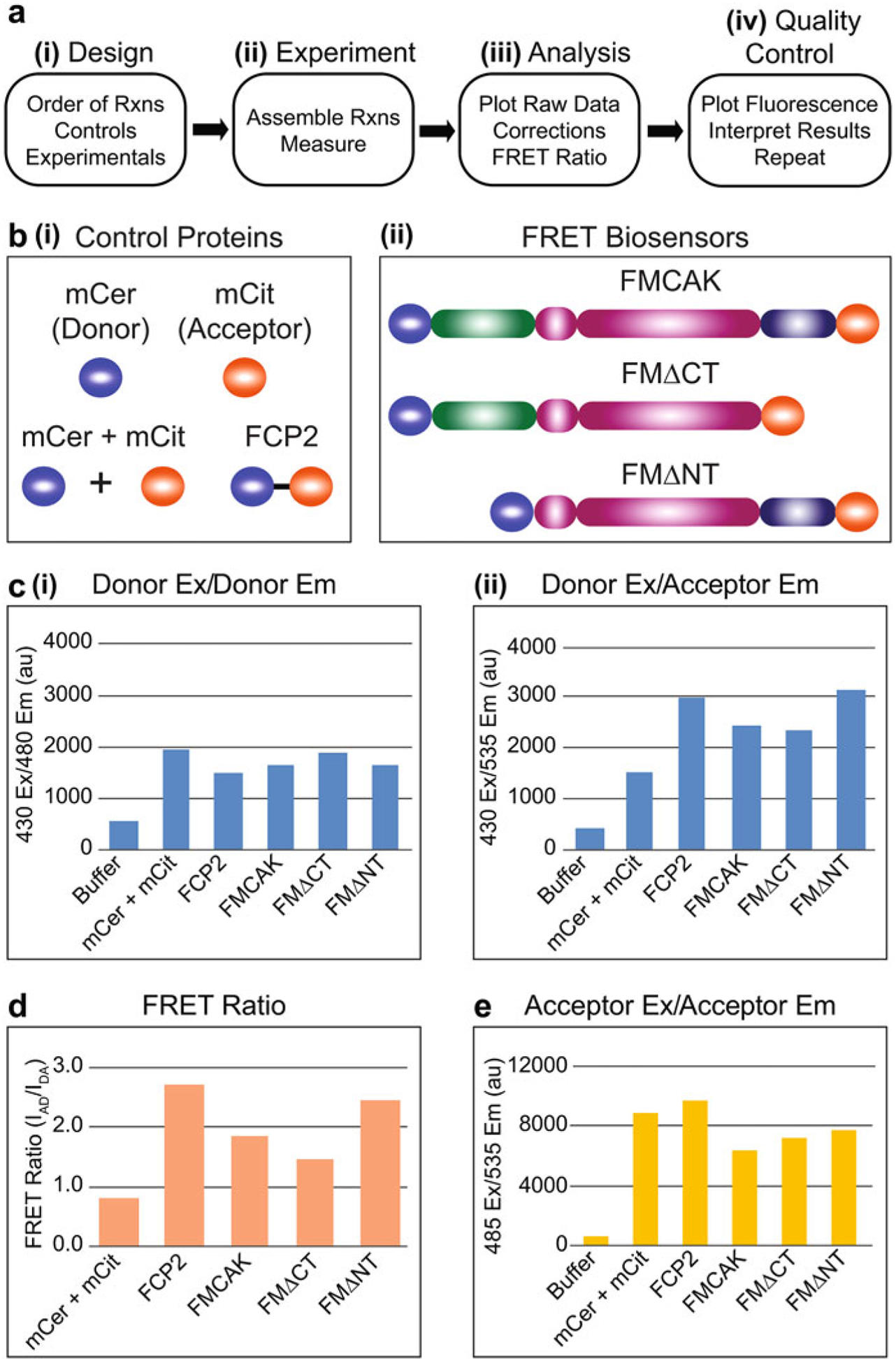
(a) Pipeline for the design, execution, analysis, and interpretation of intramolecular FRET assays to study protein conformation. (b) Schematics of negative mCerulean donor (mCer) and mCitrine acceptor (mCit) control proteins, and positive FCP2 FRET control protein (i). Schematics of FMCAK, FMΔCT, and FMΔNT FRET biosensors for full-length, CT-deleted, and NT-deleted MCAK, respectively (ii). MCAK NT (amino acids 2–186) is in green, MCAK neck and catalytic domain (amino acids 187–592) is in magenta, and MCAK CT (amino acids 593–730) is in purple. (c) Example of raw filter-based emission data of the intramolecular FRET assay in which the donor was excited at 430 nm, and the emission was measured for the donor at 480 nm (i) and for the acceptor at 535 nm (ii). (d) The background-corrected FRET ratios (I_AD/I_DA) of the data presented in (c). (e) Quality control fluorescence of the acceptor excitation and emission

MCAK in solution exists in a compact conformation in which its N-and C-termini are close together [28, 41, 42]. This closed/compact conformation can be demonstrated by FRET when the N- and C-termini are tagged with FRET pairs [28]. To understand how the N- and C-termini are involved in MCAK conformation, we generated FRET biosensors of N- and C-terminal domain truncation mutants of MCAK that we call FMΔNT and FMΔCT and compared them to full-length FRET MCAK, called FMCAK. In this example, the FRET pair is mCerulean (donor) and mCitrine (acceptor), which are derivatives of CFP and YFP, respectively. The BRB49 buffer composition used in this example was chosen to optimize FRET for downstream applications involving MT binding, which prefers high-ionic-strength solutions like PIPES.

1. Determine order and number of reactions to be added to the multi-well plate, being sure to include the appropriate controls. In this example, wells A1–6 of a 96-well half area black plate are used (see Notes 3 and 4).

2. Control reactions include (Fig. 3bi):

   1. Buffer control (reaction control buffer, well A1).
   2. Negative control donor + acceptor control proteins in reaction buffer (mCerulean + mCitrine, well A2).
   3. Positive control protein in reaction buffer (FCP2, well A3).
3. Experimental reactions include (Fig. 3bii):

   1. Full-length protein: FMCAK in reaction buffer (well A4).
   2. C-terminal domain (CT) deletion: FMΔCT in reaction buffer (well A5).
   3. N-terminal domain (NT) deletion: FMΔNT in reaction buffer (well A6).

3.3.2. Set Up and Perform the Intramolecular FRET Assay to Study Protein Conformation (Fig. 3aii)

1. Make master mixes on ice (see Note 12).

   1. Reaction buffer (24 mM KCl, 2 mM MgATP, 0.2 mg/mL casein, BRB49/DTT) (see Notes 20 and 21).
   2. Negative control proteins: 100 nM mCerulean +100 nM mCitrine in reaction buffer.
   3. Positive control protein: 100 nM FCP2 in reaction buffer.
   4. Experimental proteins: 100 nM FMCAK in reaction buffer, 100 nM FMΔNT in reaction buffer, and 100 nM FMΔCT in reaction buffer.

2. Aliquot 50 μL control buffer, negative control proteins, positive control protein, and FMCAK proteins to 96-well half-area black plate, and incubate for 10 min at RT to equilibrate.

3. Measure the following FRET components and the fluorescence of the acceptor protein sequentially per well in a plate reader based on the spectral properties of your donor and acceptor fluorophores. In this example, the fluorophores are mCerulean and mCitrine, and the reactions were read in a filter-based plate reader (see Note 10).

   1. Donor excitation and donor emission read (donor Ex/donor Em) with 430/10 nm excitation and 480/10 nm emission filters.
   2. Donor excitation and acceptor emission read (donor Ex/acceptor Em) with 430/10 excitation and 535/20 nm emission filters.
   3. Acceptor excitation and acceptor emission read (acceptor Ex/acceptor Em) with 485/10 nm excitation and 535/20 nm emission filters.

4. Export the data to Excel.

3.3.3. Analyze the Intramolecular FRET Assay to Study Protein Conformation (Fig. 3aiii)

1. Plot the raw emission of the donor Ex/donor Em and donor Ex/acceptor Em reactions (Fig. 3c). Copy the donor Ex/donor Em and donor Ex/acceptor Em read data into separate tables in Excel with appropriate column and row headers (see Note 17). Graph the donor Ex/donor Em (Fig. 3ci) and donor Ex/acceptor Em (Fig. 3cii) emission intensities in separate bar graphs, and ensure that the donor emission values are three- to fourfold higher than the buffer background levels.

2. Correct the donor Ex/donor Em and donor Ex/acceptor Em intensity values for background fluorescence. Copy the column and row headers into a new table called “Corr.” Correct the control and experimental emission intensities by subtracting the appropriate buffer-only donor Ex/donor Em or donor Ex/acceptor Em fluorescence values to account for the buffer and well background fluorescence (see Note 18). Plot corrected values in separate bar graphs and compare to the raw data. Note that the buffer emission should be zero, and the other reactions should have reduced levels from the background subtraction.

3. Calculate the FRET ratio (I_AD/I_DA) (Fig. 3d). Copy the column and row headers into a new table called “FRET Ratio.” Calculate the FRET ratio by dividing the corrected donor Ex/acceptor Em values (I_AD) by the corrected donor Ex/donor Em values (I_DA) in the “FRET Ratio” table. Graph the FRET ratios (I_AD/I_DA) according to reaction condition in a bar graph (Fig. 3d).

3.3.4. Quality Control of the Intramolecular FRET Assay to Study Protein Conformation (Fig. 3aiv)

1. Plot the acceptor Ex/acceptor Em values into a separate graph (Fig. 3e). Copy the raw acceptor Ex/acceptor Em read values into a new table in Excel with appropriate column and row headers labeled “Acc/Acc.” Plot the acceptor emission values in a bar graph (Fig. 3e).

2. The donor emission intensity in the absence of FRET should be similar for equivalent concentrations of proteins, whereas in the presence of FRET, the donor emission intensity will be less and the degree dependent on the amount of energy transfer (Fig. 3ci). For example, mCer + mCit has higher donor fluorescence than FCP2, and FMΔCT has higher fluorescence than F2MCAK and FMΔNT, which have higher FRET.

3. The acceptor emission values should also be similar for equivalent concentrations of proteins (Fig. 3e). For example, mCer + mCit and FCP2 have similar acceptor emission intensities, and FMCAK, FMΔCT, and FMΔNT have similar acceptor emission intensities.

4. Interpret results based on your quality control analysis, your predictions, or hypotheses, and then repeat for reproducibility. In this example, deleting the CT of MCAK reduced FRET relative to FMCAK, suggesting that in FMCAK the CT is near the NT in space [28]. Removing the NT increased FRET relative to FMCAK, consistent with the CT being important for the closed conformation of MCAK.

3.3.5. Adaptations to the Intramolecular FRET Assay to Study Protein Conformation

This method can be readily expanded to include the regulation of protein conformation through phosphorylation by incubating with kinase or through protein-protein interactions by performing FRET in the presence of serial dilutions of protein as described in the adaptations for intermolecular protein-protein interactions (Subheading 3.2.5). For example, we showed using FRET that phosphorylation of MCAK by Aurora B opens the conformation of MCAK [28]. Because FRET detection by monochromator- or filter-based reads is fast, temporal effects of phosphorylation or protein-protein interaction can also be determined.

3.4. Fluorescence-Based Determination of Protein Affinity

With the sensitivity and ease of fluorescence measurement, we sought to develop an MT-binding experiment using a fluorescence microtiter plate assay because traditional MT affinity assays involve laborious gel electrophoresis followed by Coomassie staining or Western blotting. Coomassie staining requires relatively high concentrations of proteins for detection of partial binding, and Western blotting, while more sensitive, adds additional variables due to blotting and antibody detection. Here, we describe the use of fluorescence to determine the affinity of the XCTK2 tail domain for MTs and then describe possible adaptations to this assay. The development of this assay provides faster and higher throughput of samples and easier quantification.

3.4.1. Design of the Experiment for Fluorescence-Based Determination of MT Affinity

MT affinity assays consist of combining an MT-binding protein with a range of MT concentrations, incubating for approximately 15 min to reach steady state, sedimentation of the MTs at high g-forces to separate the MT-bound and not unbound proteins, and then analyzing the supernatant and pellet fractions. In this example, we will use the XCTK2 tail domain tagged with YPet, YPet-XTail.

1. Determine order and number of reactions, being sure to include appropriate control reactions. The rotor we use in this assay has 20 positions for tubes, and we typically use 10 positions per protein for each concentration range of MTs. Thus, one rotor can accommodate two sets of MT concentrations if desired. In this example, we will only do one concentration range.

2. Control reactions include:

   1. YPet-XTail without MTs (tube #1). YPet-XTail without MTs will be used to background subtract the amount of YPet-XTail that sediments nonspecifically in the absence of MTs.
   2. Input reaction of protein plus MT buffer that will not be sedimented in the centrifuge (tube #11). The Input reaction will serve as a control for the reaction components sticking to the centrifuge tubes or loss due to sedimentation and resuspension of the pellet.

3. Experimental reactions include YPet-XTail mixed with a concentration series of MTs (tubes #2–10).

3.4.2. Set Up and Perform the Fluorescence-Based Determination of MT Affinity Experiment (fig. 4aii)

Fig. 4.

(a) Pipeline for the design, execution, analysis, and interpretation of a fluorescence-based assay to determine MT-binding affinity. (b) Amount of YPet-XTail bound to increasing concentrations of MTs that was corrected for nonspecific pelleting in the absence of MTs and then plotted and fit to the quadratic nonlinear regression model for total protein binding in GraphPad Prism. (c) Quality control fluorescence of the total YPet-XTail (S + P) and Input in each reaction from (b)

1. Make fresh: BRB80/DTT and BRB80/CaCl₂, place on ice; and BRB80/DTT/Taxol, place at RT (see Note 12).

2. Polymerize MTs [43] by diluting cycled tubulin to 10 μM in BRB80/DTT and then adding GMPCPP to 0.5 mM. Incubate on ice for 5 min. Polymerize MTs for 30 min at 37 °C, supplementing with 200 μM Taxol to a final concentration of 20 μM at 20 min and continuing incubation for an additional 10 min.

3. Sediment MTs from non-polymerized tubulin at 45,000 rpm (90,000 × g) for 10 min in an Optima TLX ultracentrifuge at 35 °C, remove the supernatant, and resuspend the pelleted MTs in a small volume of BRB80/DTT/Taxol. Store at RT (see Note 22).

4. Determine the MT concentration in terms of tubulin concentration by diluting 1 μL of MTs in 59 μL of cold BRB80/CaCl₂ and incubating on ice for 10–15 min to depolymerize the MTs. Measure the absorbance of the depolymerized MTs at 280 nm, A₂₈₀, using BRB80/CaCl₂ as a blank. Calculate the concentration of tubulin using Beer’s law with 115,000 M ⁻¹ cm⁻¹ as the extinction coefficient of tubulin.

5. Serially dilute MTs into nine concentrations using BRB80/DTT/Taxol, and store at RT (see Note 22).

6. Make master mixes (see Note 12): 1 μM YPet-XTail in 100 mM KCl, 0.4 mg/mL casein, FPLC buffer (see Notes 13 and 14), store on ice; and Resuspension Buffer (5% FPLC Buffer, 0.5 × BRB80/DTT/Taxol, 0.2 mg/mL casein), place at RT (see Note 22).

7. Move YPet-XTail master mix to RT for 3 min to equilibrate (see Note 22).

8. Aliquot 10 μL of BRB80/Taxol to the Input tube at RT (tube #11). This reaction will not be sedimented.

9. Aliquot 10 μL of BRB80/Taxol to TLA100 tube #1 at RT as a control for YPet-XTail that sediments in the absence of MTs. Aliquot 10 μL of each MT concentration in the serial dilution to the additional TLA100 tubes #2–10 at RT.

10. Add 10 μL of 1 μM YPet-XTail protein to the reaction tubes #1–10 and the Input tube #11 to start the reaction. Incubate at RT for 15 min.

11. Pellet the samples in tubes #1–10 at 45,000 rpm (90,000 g) in TLA100 rotor in an ultracentrifuge centrifuge for 10 min at 22 °C.

12. Save the supernatant in a fresh 1.5 mL tube being careful to avoid the pellet (see Note 23). Store at RT.

13. Resuspend the pellets in 20 μL resuspension buffer.

14. Move 15 μL of the supernatant and pellet samples to a 384-well black plate (see Notes 3 and 4), alternating the supernatant and pellet fractions into wells A1–A20. Ten reactions become 20 supernatant and pellet fractions. Be careful not to introduce bubbles (see Note 24).

15. Add 15 μL of the Input reaction (tube #11) to well A21 (see Note 24).

16. Spin the plate at 1000 rpm (180 × g) for 30 s in a plate centrifuge (e.g., Eppendorf 5810R) to collect the sample to the bottom of the plate.

17. Measure the acceptor fluorescence with plate reader. For YPet in this example, YPet was excited at 500 nm, and emission was read at 530 nm with a gain of 75 in a Synergy H1 plate reader (see Note 15).

18. Export data to Excel file.

3.4.3. Analyze the Experiment for Fluorescence-Based Determination of MT Affinity (Fig. 4aiii)

1. Calculate the fraction bound. Copy data from the acceptor fluorescence read into a separate sheet in Excel with appropriate column and row headers. Calculate the total protein by adding the values for corresponding supernatant and pellet fractions in an adjacent column labeled “S + P.” Determine fraction bound in a third column labeled “Fract Bound” by dividing pellet fraction by total protein.

2. Normalize the concentration of bound protein in a fourth column labeled “μM Bound” by multiplying the fraction bound by the concentration added. In this example, the concentration of protein added was 0.05 μM.

3. Correct the concentration bound for nonspecific pelleting. Copy the concentration bound to a separate table in the Excel sheet labeled with the corresponding MT concentration. Subtract the pelleted protein in the reaction without MTs in an adjacent column (see Note 18).

4. Copy the background-subtracted data to a program that can fit the data to a quadratic binding curve like GraphPad Prism (Fig. 4b).

3.4.4. Quality Control of the Fluorescence-Based Determination of MT Affinity Experiment (Fig. 4aiv)

1. Graph the total protein fluorescence values from the “S + P” column in Subheading 3.4.3, step 1, and the Input fluorescence against the MT concentration for equivalent addition of protein (Fig. 4c).

2. If the total protein of a reaction is drastically awry from the other reactions or from the Input, consider the validity of the data point and whether it should be included in the analysis or whether the experiment needs to be repeated (see Note 25). Also, if there is a dramatic increase in total protein fluorescence with increasing protein concentration indicating considerable protein loss at the lower concentrations, consider using higher amounts of protein or different blocking agents (e.g., casein or BSA) in the reactions (see Note 13).

3. Fit the data to a nonlinear regression model for binding affinity in software like GraphPad Prism. An appropriate binding curve will appear hyperbolic when plotted on a linear scale (Fig. 4b).

4. Interpret your results. Ideally, points below and above the K_d are needed to assure an accurate determination of the affinity. If the full binding curve was not represented with the concentrations of MTs used, repeat experiment with adjusted MT concentrations that would be predicted to approximate the full binding curve. Typically, concentrations range from tenfold below and above the K_d.

5. Repeat at least three times for reproducibility once a set of optimal concentrations are determined.

3.4.5. Adaptations

This assay can be easily adapted to measuring the effects of inhibitors on MT binding by adding increasing concentrations of the inhibitors as described for the intermolecular protein-protein interaction assay (Subheading 3.2.5). For example, importin α/β inhibit the binding of the XCTK2 tail domain to MTs [30] and could be added at increasing concentrations to measure inhibition quantitatively using fluorescence of the YPet-XTail domain. Furthermore, for non-sedimentation-based assays, FRET can be used as a read out for the fraction of protein binding by using the maximum FRET ratio at saturating ligand as 100% bound.

4. Notes

1. When preparing GMPCPP-stabilized MTs, it is essential that all solutions be made as potassium salts because a combination of glycerol and sodium can induce hydrolysis of GMPCPP [44], which decreases the stability of MTs stabilized with GMPCPP.

2. Measure the exact concentration of MgATP by absorbance at 259 nm using 15,400 M⁻¹ cm ⁻¹ as the extinction coefficient for ATP.

3. Black or white plates are ideal for fluorescence to prevent bleed through from adjacent wells.

4. Half area 96-well plates and 384-well plates are very convenient for smaller volumes when samples are precious or in low supply. Minimum recommended volume for half area 96-well plates is 50 and 20 μL for 384-well plates.

5. Solubility of fluorescent protein fusion proteins in bacteria can be improved by induction at a lower temperature, 16–20 °C, overnight or up to 24 h.

6. Determine the concentration of the fluorophore in the sample by measuring the absorbance at the appropriate wavelength for the fluorophore using Beer’s law and the extinction coefficient according to the equation A = l * c * ε, where A is the absorbance, l is the pathlength of the light source in cm, c is the concentration in molarity (M), and ε is the extinction coefficient in M ⁻¹ cm⁻¹.

7. Determine the concentration of your protein of interest by densitometry using a gel-based assay. Run 0.5 μg of protein, based on the Bradford and absorbance assays, on an SDS-PAGE gel with a serial dilution of BSA from 0 to 0.8 μg as a standard followed by Coomassie staining and densitometry. Run more protein on the gel if the total protein and absorbance concentrations are quite different. This may indicate a protein prep that has considerable contamination by host proteins or degradation products.

8. Typically, 50–200 nM protein is needed to get a good fluorescence signal that is at least two- to four-fold higher than the background of a well containing the same buffer as the proteins. Be aware that the donor fluorescence of the positive FRET control protein (FCP1) or the combination of the donor and acceptor FRET biosensors (CyPet-XCTK2 + importin α-YPet) is more difficult to assess because of the effects of FRET on the donor emission.

9. Note that the FRET control protein FCP1 consistently had higher acceptor fluorescence despite being added at an equal molar concentration to CyPet and YPet.

10. The three components of FRET can be measured spectrally or individually with single measurements from monochromatoror filter-based spectrophotometers. We find spectral measurements of FRET more helpful in assessing the quality of an experiment.

11. The acceptor controls are separate reactions containing the indicated acceptor protein concentrations performed in the absence of the donor. These reactions are necessary to calculate FRET in intermolecular FRET assays, because the bleed through of acceptor emission upon the excitation of the donor at each acceptor concentration must be considered in the final calculations.

12. Be sure to make enough master mix for all your control and experimental reactions plus extra to account for pipetting error.

13. We find for many proteins that adding casein or BSA stabilizes the protein by preventing loss due to nonspecific binding of the proteins to surfaces of the tubes and plates.

14. XCTK2 is purified by conventional chromatography and has a final KCl concentration of 300 mM KCl, which is nonphysio-logical and often too high for many downstream applications. It is important to have high-protein-concentration preps so that the final salt concentration in the reaction can be diluted to physiological levels. Adjust KCl concentration with 1 M KCl FPLC Buffer.

15. We found that performing a spectral read with excitation at 405 nm in the Synergy H1 with reactions containing CyPet and YPet worked better than using the optimal excitation wavelength of 435 nm for two reasons. First, spectrophotometers have a limit as to how close the emission can be read from the excitation wavelength to prevent damage to the instrument. Second, exciting at 405 nm reduced acceptor cross talk by minimizing the YPet excitation that causes bleed through to the YPet emission wavelength.

16. Correction of the donor bleed through into the acceptor emission is not necessary because this is minimal for this FRET pair and constant for each reaction since the same concentration of donor was added to each reaction.

17. For multistep analyses, it is a good idea to make clear stepwise calculations in the form of different tables within an Excel Sheet or with separate sheets within the Excel Workbook to be able to clearly follow the transformations of the data and prevent data loss. The original data file is always best left unmodified, with the raw/original data copied or saved as a new file on which calculations are done.

18. Use the “$” in front of the column letter or cell number to make the subtracted term static for the column or cell for ease of copying to multiple columns. For example, =‘Spectra’! B2 − ‘Spectra’!$B2 will make the column letter static, and = ‘Spectra’!F2 −’Spectra’!F$6 will make the cell number static.

19. Note that the acceptor-only controls will have the returned value of #DIV/0! because the values are zero in these cells.

20. FMCAK is purified by conventional chromatography with a final concentration of 370 mM KCl. This is not physiological and can interfere with downstream applications. Use a concentrated stock of KCl, e.g., 3 M KCl, to adjust KCl concentration depending on the stock protein concentrations.

21. Some proteins are more stable in the specific nucleotide states. MCAK is most stable in the ATP-bound state; thus, MgATP is added to the reaction.

22. It is important not to induce MT depolymerization by incubating MTs on ice or adding cold buffers to solutions containing MTs. Store MTs at RT.

23. It is convenient to place a mark on the rim of the TLA100 tube, and then place this mark to the outside of the rotor to indicate where the pellet will be as the pellets are small and hard to see.

24. Avoid introducing bubbles by consistently and gently pipetting the sample three times and then adding the sample into the plate by dispensing to the first stop of the Pipetman.

25. It is not uncommon for the total protein fluorescence to increase with increasing concentrations of MTs due to stabilization of the protein by binding to the MTs or by the presence of additional protein in the reaction.

References

- 1.Prosser SL, Pelletier L (2017) Mitotic spindle assembly in animal cells: a fine balancing act. Nat Rev Mol Cell Biol 18:187–201 [DOI] [PubMed] [Google Scholar]
- 2.Yount AL, Zong H, Walczak CE (2015) Regulatory mechanisms that control mitotic kinesins. Exp Cell Res 334:70–77 [DOI] [PMC free article] [PubMed] [Google Scholar]
- 3.Sahoo H (2011) Förster resonance energy transfer—a spectroscopic nanoruler: principle and applications. J Photochem Photobiol C 12:20–30 [Google Scholar]
- 4.Clegg RM (2009) Förster resonance energy transfer—FRET what is it, why do it, and how it’s done In: Gadella TWJ (ed) FRET and FLIM techniques, 1st edn Elsevier, Boston, MA, pp 1–57 [Google Scholar]
- 5.Selvin PR (1995) Fluorescence resonance energy transfer. Methods Enzymol 246:300–334 [DOI] [PubMed] [Google Scholar]
- 6.Stryer L, Haugland RP (1967) Energy transfer: a spectroscopic ruler. Proc Natl Acad Sci U S A 58:719–726 [DOI] [PMC free article] [PubMed] [Google Scholar]
- 7.Förster T (1948) Zwischenmolekulare energiewanderung und fluoreszenz. Ann Phys 437:55–75 [Google Scholar]
- 8.Lakowicz JR (2006) Principles of fluorescence spectroscopy, 3rd edn Springer Science, New York [Google Scholar]
- 9.Kaláb P, Pralle A (2008) Quantitative fluorescence lifetime imaging in cells as a tool to design computational models of Ran-regulated reaction networks. Methods Cell Biol 89:541–568 [DOI] [PubMed] [Google Scholar]
- 10.Raghav D, Sebastian J, Rathinasamy K (2018) Biochemical and Biophysical characterization of curcumin binding to human mitotic kinesin Eg5: Insights into the inhibitory mechanism of curcumin on Eg5. Int J Biol Macromol 109:1189–1208 [DOI] [PubMed] [Google Scholar]
- 11.Kaan HY, Major J, Tkocz K et al. (2013) “Snapshots” of ispinesib-induced conformational changes in the mitotic kinesin Eg5. J Biol Chem 288:18588–18598 [DOI] [PMC free article] [PubMed] [Google Scholar]
- 12.Hopkins SC, Vale RD, Kuntz ID (2000) Inhibitors of kinesin activity from structure-based computer screening. Biochemistry 39:2805–2814 [DOI] [PubMed] [Google Scholar]
- 13.Umezu N, Umeki N, Mitsui T et al. (2011) Characterization of a novel rice kinesin O12 with a calponin homology domain. J Biochem 149:91–101 [DOI] [PubMed] [Google Scholar]
- 14.Bajar BT, Wang ES, Zhang S et al. (2016) A guide to fluorescent protein FRET pairs. Sensors (Basel) 16:1–24 [DOI] [PMC free article] [PubMed] [Google Scholar]
- 15.Verbrugge S, Lansky Z, Peterman EJ (2009) Kinesin’s step dissected with single-motor FRET. Proc Natl Acad Sci U S A 106:17741–17746 [DOI] [PMC free article] [PubMed] [Google Scholar]
- 16.Martin DS, Fathi R, Mitchison TJ et al. (2010) FRET measurements of kinesin neck orientation reveal a structural basis for processivity and asymmetry. Proc Natl Acad Sci U S A 107:5453–5458 [DOI] [PMC free article] [PubMed] [Google Scholar]
- 17.Hajdo L, Skowronek K, Kasprzak AA (2004) Spatial relationship between heads of dimeric Ncd in the presence of nucleotides and microtubules. Arch Biochem Biophys 421:217–226 [DOI] [PubMed] [Google Scholar]
- 18.Aoki T, Tomishige M, Ariga T (2013) Single molecule FRET observation of Kinesin-1’s head-tail interaction on microtubule. Biophysics (Nagoya-shi) 9:149–159 [DOI] [PMC free article] [PubMed] [Google Scholar]
- 19.Mori T, Vale RD, Tomishige M (2007) How kinesin waits between steps. Nature 450:750–754 [DOI] [PubMed] [Google Scholar]
- 20.Shaner NC, Steinbach PA, Tsien RY (2005) A guide to choosing fluorescent proteins. Nat Methods 2:905–909 [DOI] [PubMed] [Google Scholar]
- 21.Wagner OI, Esposito A, Kohler B et al. (2009) Synaptic scaffolding protein SYD-2 clusters and activates kinesin-3 UNC-104 in C. elegans. Proc Natl Acad Sci U S A 106:19605–19610 [DOI] [PMC free article] [PubMed] [Google Scholar]
- 22.Cai D, Hoppe AD, Swanson JA et al. (2007) Kinesin-1 structural organization and conformational changes revealed by FRET stoichiometry in live cells. J Cell Biol 176:51–63 [DOI] [PMC free article] [PubMed] [Google Scholar]
- 23.Espenel C, Acharya BR, Kreitzer G (2013) A biosensor of local kinesin activity reveals roles of PKC and EB1 in KIF17 activation. J Cell Biol 203:445–455 [DOI] [PMC free article] [PubMed] [Google Scholar]
- 24.Hackney DD, Baek N, Snyder AC (2009) Half-site inhibition of dimeric kinesin head domains by monomeric tail domains. Biochemistry 48:3448–3456 [DOI] [PMC free article] [PubMed] [Google Scholar]
- 25.Hallen MA, Liang ZY, Endow SA (2011) Two-state displacement by the Kinesin-14 Ncd stalk. Biophys Chem 154:56–65 [DOI] [PMC free article] [PubMed] [Google Scholar]
- 26.Kaláb P, Soderholm J (2010) The design of Förster (fluorescence) resonance energy transfer (FRET)-based molecular sensors for Ran GTPase. Methods 51:220–232 [DOI] [PMC free article] [PubMed] [Google Scholar]
- 27.Hao Y, Macara IG (2008) Regulation of chromatin binding by a conformational switch in the tail of the Ran exchange factor RCC1. J Cell Biol 182:827–836 [DOI] [PMC free article] [PubMed] [Google Scholar]
- 28.Ems-McClung SC, Hainline SG, Devare J et al. (2013) Aurora B inhibits MCAK activity through a phosphoconformational switch that reduces microtubule association. Curr Biol 23:2491–2499 [DOI] [PMC free article] [PubMed] [Google Scholar]
- 29.Walczak CE, Verma S, Mitchison TJ (1997) XCTK2: A kinesin-related protein that promotes mitotic spindle assembly in Xenopus laevis egg extracts. J Cell Biol 136:859–870 [DOI] [PMC free article] [PubMed] [Google Scholar]
- 30.Ems-McClung SC, Zheng Y, Walczak CE (2004) Importin α/β and Ran-GTP regulate XCTK2 microtubule binding through a bipartite nuclear localization signal. Mol Biol Cell 15:46–57 [DOI] [PMC free article] [PubMed] [Google Scholar]
- 31.Basics of FRET Microscopy (2019) MicroscopyU: the source for microscopy education. https://www.microscopyu.com/applications/fret/basics-of-fret-microscopy. Accessed 16 Apr 2019 [Google Scholar]
- 32.Lambert TJ (2019) FPbase: a community-editable fluorescent protein database. Nat Methods 16:277–278 [DOI] [PubMed] [Google Scholar]
- 33.Fluorescence SpectraViewer (2019) https://www.thermofisher.com/us/en/home/life-science/cell-analysis/labeling-chemistry/fluorescence-spectraviewer.html. Accessed 16 Apr 2019 [Google Scholar]
- 34.Shimozono S, Miyawaki A (2008) Engineering FRET constructs using CFP and YFP. Methods Cell Biol 85:381–393 [DOI] [PubMed] [Google Scholar]
- 35.Nguyen AW, Daugherty PS (2005) Evolutionary optimization of fluorescent proteins for intracellular FRET. Nat Biotechnol 23:355–360 [DOI] [PubMed] [Google Scholar]
- 36.Thaler C, Koushik SV, Blank PS et al. (2005) Quantitative multiphoton spectral imaging and its use for measuring resonance energy transfer. Biophys J 89:2736–2749 [DOI] [PMC free article] [PubMed] [Google Scholar]
- 37.Koushik SV, Chen H, Thaler C et al. (2006) Cerulean, Venus, and VenusY67C FRET reference standards. Biophys J 91:L99–L101 [DOI] [PMC free article] [PubMed] [Google Scholar]
- 38.Guillaud L, Wong R, Hirokawa N (2008) Disruption of KIF17-Mint1 interaction by CaMKII-dependent phosphorylation: a molecular model of kinesin-cargo release. Nat Cell Biol 10:19–29 [DOI] [PubMed] [Google Scholar]
- 39.Kaláb P, Weis K, Heald R (2002) Visualization of a Ran-GTP gradient in interphase and mitotic Xenopus egg extracts. Science 295:2452–2456 [DOI] [PubMed] [Google Scholar]
- 40.Wang E, Ballister ER, Lampson MA (2011) Aurora B dynamics at centromeres create a diffusion-based phosphorylation gradient. J Cell Biol 194:539–549 [DOI] [PMC free article] [PubMed] [Google Scholar]
- 41.McHugh T, Zou J, Volkov VA et al. (2019) The depolymerase activity of MCAK shows a graded response to Aurora B kinase phosphorylation through allosteric regulation. J Cell Sci 132:1–8 [DOI] [PMC free article] [PubMed] [Google Scholar]
- 42.Talapatra SK, Harker B, Welburn JP (2015) The C-terminal region of the motor protein MCAK controls its structure and activity through a conformational switch. Elife 4:1–21 [DOI] [PMC free article] [PubMed] [Google Scholar]
- 43.Desai A, Walczak CE (2001) Assays for microtubule destabilizing kinesins In: Vernos I (ed) Kinesin protocols, vol 164 Humana Press, Totowa, NJ, pp 109–121 [DOI] [PubMed] [Google Scholar]
- 44.Caplow M, Ruhlen RL, Shanks J (1994) The free energy for hydrolysis of a microtubule-bound nucleotide triphosphate is near zero: all of the free energy for hydrolysis is stored in the microtubule lattice. J Cell Biol 127:779–788 [DOI] [PMC free article] [PubMed] [Google Scholar]