A neural network for online spike classification that improves decoding accuracy

Abstract

Separating neural signals from noise can improve brain-computer interface performance and stability. However, most algorithms for separating neural action potentials from noise are not suitable for use in real time and have shown mixed effects on decoding performance. With the goal of removing noise that impedes online decoding, we sought to automate the intuition of human spike-sorters to operate in real time with an easily tunable parameter governing the stringency with which spike waveforms are classified. We trained an artificial neural network with one hidden layer on neural waveforms that were hand-labeled as either spikes or noise. The network output was a likelihood metric for each waveform it classified, and we tuned the network’s stringency by varying the minimum likelihood value for a waveform to be considered a spike. Using the network’s labels to exclude noise waveforms, we decoded remembered target location during a memory-guided saccade task from electrode arrays implanted in prefrontal cortex of rhesus macaque monkeys. The network classified waveforms in real time, and its classifications were qualitatively similar to those of a human spike-sorter. Compared with decoding with threshold crossings, in most sessions we improved decoding performance by removing waveforms with low spike likelihood values. Furthermore, decoding with our network’s classifications became more beneficial as time since array implantation increased. Our classifier serves as a feasible preprocessing step, with little risk of harm, that could be applied to both off-line neural data analyses and online decoding.

NEW & NOTEWORTHY Although there are many spike-sorting methods that isolate well-defined single units, these methods typically involve human intervention and have inconsistent effects on decoding. We used human classified neural waveforms as training data to create an artificial neural network that could be tuned to separate spikes from noise that impaired decoding. We found that this network operated in real time and was suitable for both off-line data processing and online decoding.

INTRODUCTION

Brain computer interfaces (BCIs) have been used as both research tools to understand neural phenomena (Chase et al. 2012; Golub et al. 2015; Sadtler et al. 2014; Schafer and Moore 2011) and devices to improve patient control of prosthetics (Collinger et al. 2013; Hochberg et al. 2012; Velliste et al. 2008). BCIs interpret neural signals arising from electrodes implanted in the cortex with real-time decoding algorithms; however, their performance is limited by the difficulty of isolating the activity of individual neurons from extracellular voltage signals (“spike-sorting”), the characteristics of the information present in individual neurons and multiunit activity (their “tuning”), as well as the nuances of interactions among neurons (Averbeck et al. 2006). Refining the raw data is necessary to improve BCI performance, but identifying waveforms that contain relevant information is challenging.

One common noise removal method is to use all waveforms crossing a minimum voltage threshold for decoding, where all waveforms on a particular channel are considered to be from a single neural “unit” (Christie et al. 2015; Lewicki 1998). Using threshold crossings also serves to reduce the amount of stored data. However, threshold crossings often capture noise and the summed activity of multiple nearby neurons, called multiunit activity, on each channel (Rey et al. 2015; Stark and Abeles 2007). Alternatively, since waveforms with the characteristic shape of an action potential are the focus of most off-line neural data analyses, a different approach is to isolate well-defined spike waveforms from the threshold crossings via spike-sorting and use only those waveforms for decoding (Lewicki 1998; Rey et al. 2015). Unfortunately, most spike-sorting techniques are unsuitable for BCI use because they are time intensive and require manual refinement.

Furthermore, even with the development of real-time, automated spike-sorting algorithms (Chaure et al. 2018; Chung et al. 2017), deciding which waveforms should be used by the decoding algorithm is challenging. There is typically no clear ground truth for what constitutes a spike waveform based solely on sparse extracellular recordings (Pedreira et al. 2012; Rey et al. 2015; Rossant et al. 2016; Wood et al. 2004), except in the case of a few rare data sets (Anastassiou et al. 2015; Neto et al. 2016). Although some studies have found that spike-sorted units improved decoding performance (Kloosterman et al. 2014; Santhanam et al. 2004; Todorova et al. 2014; Ventura and Todorova 2015), others have found that using pooled spikes from threshold crossings resulted in comparable or better decoding that was more stable over time (Chestek et al. 2011; Christie et al. 2015; Dai et al. 2019; Fraser et al. 2009; Gilja et al. 2012). These conflicting results highlight the gap in our understanding of what information in neural recordings is most valuable for BCIs. Even within studies, there are inconsistent effects of spike-sorting on decoding, both between subjects and over time (Christie et al. 2015; Fraser et al. 2009). It is also difficult to compare the effects of spike-sorting on decoding performance across studies because of the inherent variability in spike-sorting techniques (Pedreira et al. 2012; Rey et al. 2015; Rossant et al. 2016; Wood et al. 2004) and differences in brain regions, parameters being studied, and decoding algorithms that may influence which waveforms are the most decodable (Bishop et al. 2014; Chestek et al. 2011; Fraser et al. 2009; Lewicki 1998; Oby et al. 2016). Furthermore, it is unclear whether spike-sorting, where the goal is to define isolated single units, is the best-suited approach for preprocessing data for decoding, where multiunit activity has been shown to be sufficient in some cases (Stark and Abeles 2007).

Given spike-sorting’s history of variable effects on decoding performance, we sought to avoid explicitly sorting our data and instead developed an easily tunable spike classifier that could objectively and efficiently assign waveforms to one of two classes: spike or noise. To achieve this goal, we sought a classification approach that 1) would take advantage of the spike-sorted waveforms from previous analyses that formed a readily available, labeled training data set; 2) would output a likelihood of being a spike for each waveform so we could simply adjust the minimum cutoff for binary spike classification; and 3) once trained could operate in real time. We built a neural network classifier that satisfied these three criteria. To evaluate our classifier’s performance, we decoded the activity of sparse electrode arrays implanted in prefrontal cortex (PFC) and compared decoding accuracy of task condition with all threshold crossings to decoding accuracy with the waveforms selected by our classifier. We also assessed how decoding performance changed as a function of the stringency of our classifier (i.e., the minimum cutoff for spike classification) and explored how decoding accuracy with our classifier changed as a function of time since the array implantation (array implant age).

By removing waveforms that the network identified as unlikely to be spikes, we improved decoding performance for most sessions relative to decoding with all threshold crossings. Moreover, in the remaining sessions there was no substantial detriment to decoding accuracy, meaning we could apply our method with little risk of harming decoding performance. Our network classifications continued to improve decoding accuracy in sessions recorded long after array implantation, even though the overall decoding accuracy decreased and the array recordings became noisier. Thus our real-time, tunable waveform classifier demonstrates promise for long-term BCI applications and for efficient off-line preprocessing.

MATERIALS AND METHODS

We trained a neural network, using a database of spike-sorted waveforms, to assign waveforms to a spike or noise class. We then tested the network’s classifications with another data set that was independent from the training set. In contrast to the off-line, human-supervised spike-sorting that was used to label the training data, our network did not sort waveforms into isolated single units but rather assigned spike or noise classifications to individual waveforms (hence its name, Not A Sorter, or NAS). To evaluate the network’s classifications, we decoded task location using only waveforms labeled as spikes by the network and compared the accuracy to decoding accuracy using all threshold crossings. All experimental procedures were approved by the Institutional Animal Care and Use Committee of the University of Pittsburgh and were performed in accordance with the National Institutes of Health Guide for the Care and Use of Laboratory Animals.

Neural recordings.

We analyzed neural recordings from six adult male rhesus macaques (Macaca mulatta) that had previously been spike-sorted for ongoing experiments in the laboratory. Data from four subjects were used to train our spike-classifying neural network, and data from the remaining two subjects (monkey Pe and monkey Wa) were used to assess decoding accuracy with the network’s classifications. Raw recordings from both 96-electrode “Utah” arrays (Blackrock Microsystems, Salt Lake City, UT) and 16-channel linear microelectrode arrays (U-Probe; Plexon, Dallas, TX) were band-pass filtered from 0.3 to 7,500 Hz, digitized at 30 kHz, and amplified by a Grapevine system (Ripple, Salt Lake City, UT). The interelectrode distance on the Utah arrays was 400 μm and that on the linear arrays was 150 or 200 μm, beyond the range over which the two extracellular electrodes are likely to capture the waveform of a single neuron. For each recording session, a threshold (V_T) was defined for each channel independently based on the root-mean-squared voltage of the waveforms (V_RMS) recorded on that channel at the beginning of the session (i.e., V_T = V_RMS × X, where X was a multiplier set by the experimenter). Each time the signal crossed that threshold, a 52-sample waveform segment was captured (i.e., a threshold crossing), with 15 samples before and 36 samples after the sample in which the threshold excursion occurred.

Off-line spike-sorting.

All data in this work were spike-sorted to identify well-defined single units for previous studies. These presorted data were used to create the labeled training set for this study. Waveform segments were initially sorted into spike units and noise with a custom, off-line MATLAB spike-sorting algorithm that used an automated competitive mixture decomposition method (Shoham et al. 2003). These automated classifications for each recording session were subsequently refined manually by a researcher using custom MATLAB software (available at https://github.com/smithlabvision/spikesort). The researcher modified the classifications on each channel based on visualization of the overlaid waveform clusters, projections of the waveforms in principal component analysis (PCA) space (to assess how many clusters were present), the interspike interval distribution of any potential single unit (ensuring that it contained few waveforms separated by less than a sensible refractory period), and whether each potential single unit was stationary (i.e., present for the majority of the recording session). Although only a single researcher spike-sorted the waveforms from any particular session, the data in the training set (7 sessions total) collectively consisted of data spike-sorted by four different researchers. If multiple unique spike waveform shapes were present on a channel, the sorter would label those as different units.

Training data set.

We sought a diverse neural waveform training set that captured a variety of subjects, brain regions, implanted array ages (i.e., number of days since the array was implanted), and recording devices (Table 1). The four training data set subjects each had a 96-electrode Utah array implanted in right or left hemisphere visual area V4. Two of those subjects also had 16-channel U-Probe recordings from the frontal eye field (FEF), located in the anterior bank of the arcuate sulcus. Data from two sessions were used for three of the subjects: one session recorded shortly after the array implant and one session recorded at least 4 mo later. For the fourth subject, only a single recording session recorded shortly after the array implant was used because there were no later recordings from that array. These recordings were collected and sorted as part of previous studies that describe the experimental preparations in detail (Khanna et al. 2019; Snyder et al. 2015; Snyder and Smith 2015). Data in the training set were assigned a label of 0 or 1. If multiple single units were identified by the sorter on a particular channel, they were not distinguished in the training set and all were treated as spike waveforms (labeled as 1). We only included data from channels with very distinct spike waveforms, defined as channels with a signal-to-noise ratio (SNR) > 2.5 (Kelly et al. 2007). These channels still included both noise (labeled as 0) and spike (labeled as 1) waveforms. The aim of using only the high-SNR channels in the training set was to emphasize relatively well-isolated single-unit action potential shapes while also exposing the network to a variety of noise waveforms. Additionally, excluding low-SNR channels resulted in a training set with a relatively even distribution of spike and noise waveforms (47.5% spikes, 52.5% noise).

Table 1.

Training data set information: time since implant (array age), brain area, and number of recording sessions

	Recording Device	Brain Area	Time Since Implant	No. of Sessions
Monkey Wi	Utah array	RH V4	~1 mo	1
	Utah array	RH V4	~11 mo	1
	U-Probe	RH FEF		1
Monkey Ro	Utah array	LH V4	<1 mo	1
	Utah array	LH V4	~8 mo	1
	U-Probe	LH FEF		1
Monkey Bo	Utah array	RH V4	<1 mo	1
	Utah array	RH V4	~4 mo	1
Monkey Bu	Utah array	RH V4	~1 mo	1

Utah arrays contained 96 channels, and U-Probes had 16 channels. FEF, frontal eye field; LH, left hemisphere; RH, right hemisphere.

Overall, the network training set consisted of 24,810,795 waveforms from four monkeys, two brain regions (V4 and FEF), two recording devices (Utah array and U-Probe), and different array implant ages. These waveforms were classified as spikes or noise with the off-line spike-sorting technique described above (Fig. 1A).

Fig. 1.

Methods of classifying waveforms: classic (manual) spike-sorting and our neural network spike classifier, Not A Sorter (NAS). A: spike-sorted channels with waveforms that were manually classified as spikes and noise. The network was trained on 24,810,795 spike-sorted neural waveforms from 4 monkeys. The waveforms were recorded on arrays implanted in V4 as well as U-Probes placed in the frontal eye field. B: neural network structure and output for 3 sample waveforms. Each s = 52 waveforms input (I) was passed through a hidden layer (II) with n = 50 units. The resultant linear weighting of the waveform voltages was passed through a rectified linear unit (ReLU) nonlinearity (III). The output was again passed through a weighted sum (IV) followed by a sigmoid nonlinearity (V). The resulting value was the network’s assessment of the likelihood that the input waveform was a spike waveform (VI). We refer to this value as P(spike) or the “probability” of being a spike.

Testing data set.

We used recordings from two additional subjects, not included in the training set, for testing to ensure that the trained network was generalizable to subjects not included in its training. The two testing data set subjects (monkey Pe and monkey Wa) each had two 96-electrode Utah arrays implanted, one in visual area V4 and one in dorsolateral PFC (on the prearcuate gyrus just medial to the principal sulcus, area 8Ar). Both arrays were implanted in the right hemisphere for monkey Pe and in the left hemisphere for monkey Wa. Only data recorded from PFC were used for the complete set of analyses (Table 2) because this provided a matched data set from two monkeys for the purpose of assessing the impact of our method on decoding and because it allowed us to test our network’s generalizability in situations in which the data were recorded from a region different from the training set. However, we repeated some of the analyses in held-out data from V4 and similarly found an improvement in decoding with our network (Supplemental Fig. S5; all Supplemental Material is available at https://doi.org/10.6084/m9.figshare.11808492.v1). Recordings within 50 days of the array implant were considered early sessions, and recordings from >50 days after the implant were considered late sessions (see Table 2 for session counts by subject). For monkey Pe, the thresholds across channels were similar for all recording sessions (90% of channels had thresholds between −39 and −20 μV, median: −29 μV). For monkey Wa, the thresholds were more permissive for the later recording sessions (>6 mo after the array implant) as the experimenters sought to extract the maximum remaining signal in arrays that were decreasing in recording quality. The median threshold of monkey Wa’s early sessions was −32 μV (90% between −43 and −23 μV), and the median threshold of the later sessions was −15 μV (90% between −29 and −12 μV). The waveforms in the testing data set were also spike-sorted off-line via the technique described above for a comparative analysis between our network classifications and off-line spike-sorting.

Table 2.

Testing data set information: time since implant (array age), brain area, and number of recording sessions

	Recording Device	Brain Area	Time Since Implant	No. of Sessions
Monkey Pe	Utah array	RH PFC	11–43 days	14
		RH PFC	80–147 days	22
Monkey Wa	Utah array	LH PFC	27–40 days	5
		LH PFC	180–224 days	11

LH, left hemisphere; PFC, prefrontal cortex; RH, right hemisphere.

Neural network.

Using TensorFlow (Abadi et al. 2016) and Keras (Chollet 2015), we developed a neural network to classify data segments as spike or noise waveforms (Fig. 1B). The network accepts a waveform segment with s samples (s = 52), which passes through a hidden layer with n units (n = 50) that uses a rectified linear unit (ReLU) activation function. The product of the hidden layer passes through one output unit, and then the network applies a sigmoid function to its output.

With the aforementioned training waveforms, the network was trained to maximize accuracy based on binary labels (0 for noise, 1 for spikes) with an Adam optimization algorithm (Kingma and Ba 2015) and a binary cross-entropy loss function in batch sizes of 100.

For a single waveform input run through the trained network, the output was a value between 0 (likely not a spike) and 1 (likely a spike), which represented the network’s assessment of the likelihood that the input waveform was a spike. Although this output value was not a conventional probability, we refer to it as the probability of being a spike or P(spike) because it was a likelihood metric scaled between 0 and 1. Supplemental Fig. S1 provides more intuition regarding the hidden layer units and how the network assessed waveforms. To classify the waveforms using the network’s output probability, we set a minimum P(spike) for a waveform to be classified as a spike. We referred to this minimum probability as the γ-threshold. A γ-threshold of 0 classified all of the waveforms that were captured for the session as spikes; this is often referred to as “threshold crossings” in the literature. Increasing γ resulted in fewer waveforms classified as spikes because the P(spike) cutoff was higher.

We refer to our neural network as Not A Sorter (NAS) because it classifies waveforms as spikes or noise but does not attempt to sort the spikes into separable single units. Custom Python and MATLAB scripts used to train the neural network and classify waveforms, as well as sample training and testing data, are available at https://doi.org/10.6084/m9.figshare.11808492.v1. The NAS software is also integrated into our custom MATLAB “Spikesort” package (https://github.com/smithlabvision/spikesort).

Memory-guided saccade task.

The two testing data set subjects (monkey Pe and monkey Wa) performed a memory-guided saccade task (Fig. 2A). Each subject fixated on a central point for 200 ms. Then, a target stimulus flashed at a set amplitude and direction for 50 ms, followed by a 500-ms delay. There were a total of 40 possible conditions: the radius could be one of five eccentricities and the target direction could be one of eight (spaced in 45° steps). After the delay, the fixation point disappeared, instructing the subject to make a saccade to the location where the target flashed. For some sessions, during the saccade the target reappeared to help the subject; however, for all analyses we only used data from the beginning of the delay period (i.e., before the saccade). Subjects were rewarded with water or juice for making a saccade to the correctly remembered target location. For all decoding analyses, the decoded condition was the target location. Trials at a single eccentricity (monkey Pe: 9.9°, monkey Wa: ~7.6°) were used to maximize the number of recording sessions that could be compared. Thus there were eight unique target locations to decode.

Fig. 2.

Off-line decoding of planned direction from a memory-guided saccade task. A: memory-guided saccade task. The monkey fixated on a central point. A brief stimulus flash occurred, followed by a delay period. When the fixation point turned off, the subject was required to make a saccade to the location of the previously flashed stimulus. B: decoding paradigm. The stimulus flash could occur at 8 different angles around the fixation point. A Poisson naive Bayes classifier was used to decode stimulus direction off-line using spikes recorded from a 96-electrode Utah array in prefrontal cortex 50 ms after target offset. For each recording session, we used 5-fold cross-validation, where for each fold the data were split (step 1) into a training set to create model distributions for each direction (step 2) and an independent testing set to test the accuracy of the model’s predictions (step 3). Note that the curves in step 2 do not depict actual distributions and simply represent how a Poisson decoder could use spike counts from trials in the training set to distinguish between different target conditions.

Only rewarded trials were analyzed. The number of trial repeats per condition varied over sessions. Monkey Pe had an average of 43 repeats per session (range: 25–75, SD: 17), and monkey Wa had an average of 62 repeats per session (range: 51–83, SD: 11) for each target condition.

Decoding.

To classify target direction before movement from spikes in PFC, we used a Poisson naive Bayesian decoder (Fig. 2B). All decoding analyses were performed off-line. Waveforms classified as spikes from 300 ms to 500 ms after fixation (i.e., 50 ms after stimulus offset) were used for decoding, whereas waveforms classified as noise were discarded. Each channel was considered a single decodable unit, with one exception: to calculate decoding accuracy using manual spike-sorting, if there were multiple single units identified by the manual spike-sorting method on a channel, each single unit on that channel remained separate for the purposes of decoding. Units with an average firing rate across trials below 0.25 spikes/s were discarded. We allocated training and test trials with two different methods. For one analysis, we assigned 80% of the trials from each session to the training set and the remaining 20% to the test set (see Fig. 4, A and B). For the remaining analyses, we wanted two test sets, so we used 60% of the trials for training and 20% for each of the two test sets. The two test sets allowed us to search for an optimal γ-threshold using the first test set and cross-validate this value with the second test set. Training and test data were rotated such that each trial was used for a test set only once.

Fig. 4.

Using Not A Sorter (NAS) spike classifications improved decoding accuracy in many sessions. A and B: % decoding accuracy (black line) and % of waveforms removed (maroon line) at different γ-thresholds for an example recording session in monkeys Pe (A) and Wa (B). Chance decoding accuracy was 12.5% (verified by computing a decoding control with shuffled test trials, gray line). The decoding accuracy increased for low γ-thresholds and then reached an asymptote as γ increased. At the highest γ-thresholds, decoding accuracy fell to chance (gray line). Other labeled relevant metrics include decoding accuracy with threshold crossings (blue dot), maximum decoding accuracy (green dot), γ-threshold with the maximum decoding accuracy (gray dotted line), and Δ % decoding accuracy (the difference for a given session between the decoding accuracy using the network classifications at a particular γ-threshold and the decoding accuracy with threshold crossings). C and D: distribution of γ-thresholds across sessions [monkey Pe (C): n = 36, monkey Wa (D): n = 16] that resulted in the maximum decoding accuracy for each session. E and F: distribution of Δ % decoding accuracy across all sessions where the γ-threshold was the median from the distributions in C and D. Mean Δ % decoding accuracy is shown in red. For both monkeys, using spikes classified by the network improved decoding accuracy on average across sessions; however, this improvement was only statistically significant for monkey Pe [2-tailed Wilcoxon-signed rank test, monkey Pe (E): P < 0.0001, monkey Wa (F): P = 0.057].

Our decoding algorithm created a Poisson distribution model for each target location (θ) using the average spike count for each unit (n_spike) in the training set. For each test trial, the target location with the maximum prediction probability, P(θ|n_spike), was the predicted label. In Eq. 1, P(n_spike|θ) is calculated with the Poisson model developed with the training trials:

$$P\left(\text{θ}|n_{\text{spike}}\right)=\frac{P\left(n_{\text{spike}}|\text{θ}\right)\times P\left(\text{θ}\right)}{P\left(n_{\text{spike}}\right)}$$

Decoding accuracy was calculated as the ratio of the number of correct prediction labels to the total number of predictions. We used 5-fold cross-validation and computed the average decoding accuracy across folds.

RESULTS

We trained a one-layer neural network called Not a Sorter (NAS) to evaluate the likelihood that a neural waveform was a spike. We used a diverse set of waveforms in the training set from different brain regions, subjects, and array implant ages (time since array implant) to expose the network to a variety of waveform types. Each waveform in the training set was assigned a binary label of noise (0) or spike (1) via off-line spike-sorting with manual refinement by researchers. The network was also exposed to variability in spike classification due to manual sorting because different researchers sorted different sets of waveforms in the training data. The network learned to assess how spikelike a waveform was based on binary labels but itself output a continuous value between 0 and 1 for each waveform, allowing for tunable classification. We referred to this output as the probability of being a spike or P(spike). The network classified 1,000 waveforms in <1 ms on average (computed on a 2011 iMac with a 2.8 GHz Intel Core i7 processor). In a 10-ms bin, 1,000 waveforms would be the expected output of 1,000 channels each recording from a single unit with a firing rate of 100 spikes/s. Thus our network could be easily integrated to operate within real-time computing constraints. In a realistic simulation of a real-time application of our network, waveforms captured from 192 channels in a 20-ms time step could be classified in <0.1 ms on average, easily sufficient for the updating of a BCI cursor or other feedback.

Qualitative assessment of NAS classifications.

To assign each NAS-classified waveform a binary spike or noise label, we set a parameter called the γ-threshold, which was the minimum P(spike) a waveform needed to be considered a spike waveform. We found that even a low γ-threshold, such as γ = 0.20 (Fig. 3A), assigned most waveforms to classes that a human spike-sorter would deem appropriate. Most spike-sorters and spike-sorting algorithms search for waveforms with a canonical action potential shape—an initial voltage decrease followed by a sharp increase, a narrow peak, and a return to baseline. Increasing the γ-threshold to 0.70 [i.e., only waveforms assigned a P(spike) > 0.70 were considered spikes] mimicked the effect of more selective spike classification (Fig. 3B), where the percentage of spike waveforms on the channel decreased since more waveforms were placed in the noise class and the remaining spike waveforms had a clearer single-unit shape. Considering all of the waveforms from this same channel, the range of P(spike) values coincided well with our subjective impression of the match of individual waves with a canonical action potential shape (Fig. 3C), and this was also true across all channels from this array (Fig. 3D). Thus tuning the γ-threshold from low values (near 0) to high values (near 1) resulted in a shift from a more permissive to a more restrictive regime.

Fig. 3.

Classifying waveforms based on their probability of being a spike, P(spike), by setting γ, a tunable parameter. A and B: waveforms classified as spikes or noise for a sample channel in monkey Pe. The network outputs a value between 0 and 1, referred to as P(spike), for each waveform, where a value close to 1 means the network identifies that waveform as very likely to be a spike waveform. After running waveforms through the network, we set the minimum P(spike) to classify waveforms as spikes and referred to this value as the γ-threshold. Only waveforms assigned a spike probability > 0.20 (i.e., γ-threshold = 0.20) in A and > 0.70 (i.e., γ-threshold = 0.70) in B were classified as spikes. Increasing the γ-threshold by definition results in a smaller percentage of waveforms captured in the spike class. C: waveforms from the same channel in A and B colored based on their network-assigned P(spike) value. For a waveform where γ₁ < P(spike) < γ₂, the waveform would be classified as a spike when the threshold is γ₁ but would be labeled as noise for γ₂. D: similar to C except for the average of waveforms across all channels within the indicated P(spike) ranges. Modifying the γ-threshold tuned the stringency of the spike classifications. For the channel depicted in A–C the standard deviation of the waveform noise, computed with the method described in Kelly et al. (2007), was 17.1 μV.

Quantitative assessment of NAS classifications with decoding.

Although by eye the network appeared to classify waveforms reasonably well, we sought to objectively assess its performance by measuring its effect on off-line decoding accuracy. Specifically, we hypothesized that decoding using spikes classified by our network would be better than using threshold crossings. We applied our network to a set of data recorded from PFC on which the network had not been trained. First, we set the γ-threshold and discarded any waveforms with a P(spike) below the threshold. Next, we split the data into training and testing sets. We trained the decoder using the training set to decode the task condition (the remembered location, out of 8 possibilities) during the delay period of a memory-guided saccade task on each trial (see materials and methods). Then we used the trained decoder to assess decoding accuracy in the test set(s). We repeated this process for the same data set, using multiple γ-thresholds between 0 (i.e., all threshold crossings were considered spikes) and 0.95 (i.e., only waveforms assigned a 0.95 or greater probability by the network were considered spikes). Since only waveforms classified as spikes were used for decoding, as the γ-threshold increased fewer waveforms remained for decoding.

Initially, we used 80% of trials to train the decoder and the remaining to test it. We analyzed cross-validated decoding accuracy as a function of γ (sample recording sessions in Fig. 4, A and B). Chance decoding was 12.5% (1 out of 8) and was verified by computing decoding accuracy for shuffled test trials. The decoding accuracy using threshold crossings (γ = 0) for the sample recording sessions in Fig. 4, A and B, was close to chance levels for monkey Pe (12.8%) and was also low for monkey Wa (20.1%). Using the network’s classifications improved decoding accuracy relative to using threshold crossings. The peak decoding benefit of using the network’s spike classifications occurred at a low γ-threshold (monkey Pe: γ = 0.16, monkey Wa: γ = 0.16). Being very selective about the spikes used for decoding (by setting a high γ-threshold) did not have a large impact on decoding accuracy, which appeared to plateau after the peak. We found that increments of the γ-threshold did not remove the same number of waveforms. A substantial proportion of waveforms were removed at the lowest γ-threshold tested (especially in monkey Pe), and small increments of the γ-threshold as it approached a value of 1 could also result in large increases in the proportion of removed waveforms (especially notable in Fig. 4B). For reference, when we manually spike-sorted the same data off-line (see materials and methods), we discarded 89.2% of the waveforms in Fig. 4A and 71.5% of the waveforms in Fig. 4B. These values were similar to the percentage of waveforms the network removed at higher γ-thresholds.

Ideally, for the sake of simplicity during online BCI experiments, we could select a single γ-threshold and use it for all recording sessions. We wanted to find the lowest γ-threshold that improved decoding accuracy for the majority of recording sessions. We focused on lower γ-thresholds because it was a conservative approach, and because our intuition from single channels and results in example sessions (Fig. 4) showed it could have the greatest benefit for decoding. To cross-validate both our decoder and our γ-threshold selection for the remaining analyses we created two test sets for decoding (training set: 60% of trials, test set 1: 20% of trials, test set 2: 20% of trials). Our general strategy was to use test set 1 to identify a γ-threshold that optimized decoding accuracy. We then cross-validated this selection by applying the chosen γ-threshold to the data in test set 2 and computing decoding accuracy for those unseen trials.

As described above, after training the decoder for each session using the training trials, we calculated decoding accuracy with the first set of test trials at each γ-threshold. We found the maximum decoding accuracy at any γ-threshold > 0 and then searched for the lowest nonzero γ-threshold that resulted in a decoding accuracy within 99% of that maximum (Fig. 4, C and D). Since the optimal γ-threshold varied between sessions, we computed the median across sessions of these γ values and rounded it to the nearest tested value (monkey Pe: γ = 0.2, monkey Wa: γ = 0.08). We then used that median value as the γ-threshold for all sessions in the second test set and analyzed the change in decoding accuracy from decoding using threshold crossings in that same test set, which we termed ∆ % decoding accuracy (Fig. 4, E and F). Combining sessions from both animals, the average improvement in decoding accuracy was 3.9% (2-tailed Wilcoxon signed-rank test; across subjects: P < 0.0001, monkey Pe: P < 0.0001, monkey Wa: P = 0.057). Thus our network’s classifications tuned to the previously described γ-thresholds resulted in a net benefit for decoding performance across sessions compared with using threshold crossings. Although we could tune the γ-threshold for each session to maximize the decoding, our choice of a fixed γ-threshold was more consistent with the use of our network in an online decoding context, where it would be desirable to set a constant γ-threshold at the start of each session rather than tuning it as a free parameter. However, an alternative strategy would be to collect a small data set at the start of each day to find the optimal γ value and then continue experiments for the remainder of that day using the chosen value.

Given the ability of our network to improve decoding accuracy beyond that observed with threshold crossings, we took advantage of our longitudinal recordings in a fixed paradigm to understand how our network’s performance varied as a function of time. Since there is mixed evidence in the literature regarding decoding stability with long-term array implants, we were specifically interested in how the passage of time since array implant (array implant age), and concomitant degradation of recording quality, could influence our network’s performance.

Impact of array age.

First, we assessed how the overall quality of our neural data changed as a function of time. As the time since the array implant increased, the percentage of waveforms that the network assigned a very low probability of being a spike [P(spike) < 0.02] also increased (Fig. 5A; Spearman’s correlation, monkey Pe: ρ = 0.87, P < 0.0001; monkey Wa: ρ = 0.90, P < 0.0001). Conversely, the percentage of waveforms assigned higher probabilities of being a spike [P(spike) > 0.70] decreased over time (Fig. 5B; monkey Pe: ρ = −0.87, P < 0.0001; monkey Wa: ρ = −0.94, P < 0.0001). These classification changes were consistent with our qualitative observations that the arrays showed an increasing proportion of multiunit activity (relative to single-unit activity) and apparent noise over time. These changes were also reflected in our manual spike-sorting (performed off-line on the same data for previous studies, see materials and methods), where we discarded a smaller percentage of waveforms from earlier sessions that were 0–50 days after implant (mean % waveforms removed ± 1 SD, monkey Pe: 36.1 ± 8.2%; monkey Wa: 46.1 ± 12.2%) and a larger percentage in later sessions that were >50 days after implant (mean % waveforms removed ± 1 SD, monkey Pe: 87.0 ± 7.7%; monkey Wa: 77.8 ± 10.3%). We further found that the ratio of the percentage of waveforms assigned a high P(spike) to the percentage of waveforms assigned a low P(spike) by the network served as a proxy for a signal-to-noise ratio metric, and it was highly correlated with the median signal-to-noise ratio (across channels) of the array in each session (Supplemental Fig. S2). Both signal-to-noise metrics decreased over time, and the decoding accuracy with threshold crossings also decreased the longer the array had been implanted (Fig. 5C; monkey Pe: ρ = −0.86, P < 0.0001; monkey Wa: ρ = −0.69, P = 0.004).

Fig. 5.

Noise on the array increased with the age of the array while decoding accuracy decreased in monkey Pe and monkey Wa. A: % of waveforms with a P(spike) < 0.02 over time. A waveform with a P(spike) < 0.02 was one that the network found very unlikely to be a spike. The percentage of these unlikely spike waveforms increased as the array became older (Spearman’s correlation, monkey Pe: ρ = 0.87, P < 0.0001; monkey Wa: ρ = 0.90, P < 0.0001). B: % of waveforms with a P(spike) > 0.70 over time. The percentage of waveforms that the network found to be strongly spikelike decreased as the array became older (Spearman’s correlation, monkey Pe: ρ = −0.87, P < 0.0001; monkey Wa: ρ = −0.94, P < 0.0001). C: decoding accuracy with threshold crossings (i.e., γ = 0) decreased as the array aged (Spearman’s correlation, monkey Pe: ρ = −0.86, P < 0.0001; monkey Wa: ρ = −0.69, P = 0.004). D: change in % decoding accuracy with network-classified spikes relative to decoding accuracy with threshold crossings (Δ % decoding accuracy). We computed a distribution of the maximum γ-threshold (similar to Fig. 4, C and D) for sessions that were 0–50 days after array implant and used the median to set the γ-threshold before computing decoding accuracy for those sessions. We repeated this for sessions >50 days after array implant. In monkey Pe using Not A Sorter (NAS) classifications improved decoding accuracy (2-tailed Wilcoxon signed-rank test, P < 0.0001), and in monkey Wa using the classifications neither hurt nor helped decoding significantly (P = 0.09). In both subjects, the network helped decoding more in the late array sessions (>50 days after implant) compared with the early sessions (2-tailed Wilcoxon rank sum, monkey Pe: P = 0.01; monkey Wa: P = 0.01). E: mean normalized decoding accuracy across early sessions (open circles) and late sessions (filled circles) as a function of γ-threshold. Shading represents ±1 SE. Using the network classifications at any γ-threshold > 0 was more helpful for late sessions than it was for early sessions.

Given the change in distribution of the types of waveforms present during the session over time, we tried to optimize the γ-threshold based on time since array implant. We used the same method as in Fig. 4, C and D, to compute the γ-thresholds with approximately maximum decoding (within 1%), except that we calculated the median of the early sessions (recorded 0–50 days after implant) and the median of the late sessions (recorded >50 days after implant) separately. This did not prove to be a useful optimization, as the median values were similar between early and late sessions in both monkey Pe (γ_early = 0.25, γ_late = 0.18) and monkey Wa (γ_early = 0.06, γ_late = 0.08). Decoding accuracy compared with threshold crossings (∆ % decoding accuracy) was significantly increased in monkey Pe (Fig. 5D; 2-tailed Wilcoxon signed-rank test, P < 0.0001) and was not significantly helped or hurt in monkey Wa (P = 0.09). In line with the trends in signal and noise over time, the decoding accuracies from later sessions (>50 days after implant) were helped more by the network classifications in both subjects than those from earlier sessions (Fig. 5D; Wilcoxon rank sum, monkey Pe: P = 0.01; monkey Wa: P = 0.01). When we normalized the decoding accuracy at each γ-threshold by the decoding accuracy using threshold crossings for each session and separately averaged across early and late sessions, the increased benefit of using the network in the later sessions compared with the earlier sessions was clear (Fig. 5E).

Altogether, these results provide additional evidence that factors such as time since the array was implanted and signal-to-noise ratio influence decoding accuracy and affect how noise removal impacts decoding performance. Despite decreasing signal quality and increasing noise waveforms, the effect of using our network classifications for noise removal before decoding was consistent in that it was most often beneficial for decoding and at worst minimally detrimental. We confirmed that these results were not affected by poor γ-threshold selection by using the maximum decoding accuracy regardless of γ-threshold to calculate ∆ % decoding accuracy (Supplemental Fig. S3A). Our results were also not substantially influenced by variability in the number of trials across sessions (Supplemental Fig. S3B). An even simpler alternative to our network might be to adjust the voltage threshold for capturing waveforms, to make it more or less permissive. We found that increasing this threshold (making it more negative and therefore excluding the waveforms that did not exceed it) did not improve decoding performance (Supplemental Fig. S4), indicating that our network was not merely acting to exclude small-amplitude waveforms. Finally, we confirmed that our network was beneficial for decoding in data recorded from another brain region (V4) with different Utah arrays in the same sessions from the same animals in the test data set (Supplemental Fig. S5).

Comparison to spike-sorting.

In light of the inconsistent effect of spike-sorting on decoding performance in the literature (Christie et al. 2015; Dai et al. 2019; Fraser et al. 2009; Todorova et al. 2014), we sought to evaluate the relative merits of manual spike-sorting and our network classifier on decoding accuracy in our data. Our goal was to place our new method (using our network to remove noise but not sort the data) in the context of previous work that evaluated the impact of human-supervised spike-sorting on decoding. We took advantage of the off-line spike-sorting that had already been applied to these data and calculated the decoding accuracy of spike-sorted data (Fig. 6; data aggregated across subjects in the marginal histograms). Decoding using spike-sorted waveforms was better than using threshold crossings (Fig. 6, right; 2-tailed Wilcoxon signed-rank test, P < 0.0001) similar to decoding with our network classifications (Fig. 6, top; data from Fig. 5D aggregated across subjects, P < 0.0001). Our network’s classifications were at least as helpful as manual spike-sorting for decoding relative to using threshold crossings (Fig. 6, center; paired 2-tailed Wilcoxon signed-rank test, monkey Pe: P = 0.75, monkey Wa: P = 0.09). Furthermore, the automated real-time operation of our network confers a distinct advantage over manual spike-sorting.

Fig. 6.

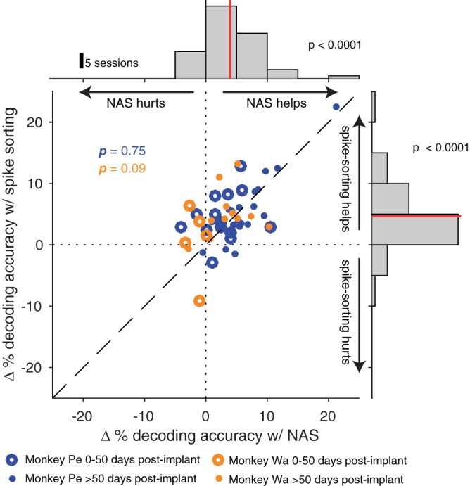
Using Not A Sorter (NAS) classifications was comparable to using spike-sorted data for decoding. Δ % decoding accuracy was calculated for both NAS classifications and spike-sorted waveforms as the change from decoding accuracy with threshold crossings. Top: distribution of Δ % decoding accuracy using NAS classifications aggregated across subjects (γ-threshold selected as in Fig. 5D). Using NAS classifications improved decoding accuracy from that with threshold crossings (2-tailed Wilcoxon signed-rank test, P < 0.0001). Right: distribution of Δ % decoding accuracy using manual spike-sorting aggregated across subjects. Using spike-sorted classifications also improved decoding accuracy from that with threshold crossings (2-tailed Wilcoxon signed-rank test, P < 0.0001). Center: the joint distribution of Δ % decoding accuracy with spike-sorting- and NAS-classified spikes. Using our network’s classifications was at least as helpful as spike-sorting for decoding (paired, 2-tailed Wilcoxon signed-rank test, monkey Pe: P = 0.75; monkey Wa: P = 0.09).

Together, our analyses demonstrate that our network was able to produce classifications of spikes and noise that matched our qualitative expectations and could be tuned quantitatively to adjust its permissiveness. Compared with using threshold crossings, our network’s classifications most often led to an improvement or minimally harmful change in decoding accuracy, indicating that there was usually little downside to the application of our network. These outcomes are valuable particularly in the context of a BCI, where real-time operation and maximal decoding accuracy are prized.

DISCUSSION

By leveraging our pool of previously spike-sorted data, we trained a neural network classifier to separate spikes from noise in extracellular electrophysiological recordings in real time. To assess the value of this method, we used an objective criterion—the ability to decode remembered location from prefrontal cortex in a memory-guided saccade task. We found that we could set a fixed γ-threshold that resulted in an improvement or at worst a small change in decoding accuracy for the majority of sessions, and this effect persisted even as recording quality decreased over time. Compared with spike-sorting (performed off-line with substantial manual labor involved), classifying spikes with our network had similar effects on decoding accuracy relative to threshold crossings and was less tedious.

Training the network.

Developing a neural network trained on spike-sorted data allowed us to capture the essence of the rules by which experienced researchers distinguish spikes from noise without explicitly defining all the variables and exceptions, a standard challenge in spike classification (Wood et al. 2004). Several studies have demonstrated the promise of using a neural network trained on spike-sorted or human-verified data for spike detection and classification (Chandra and Optican 1997; Kim and Kim 2000; Lee et al. 2017; Racz et al. 2020; Saif-ur-Rehman et al. 2019). Lee et al. (2017), Racz et al. (2020), and Saif-ur-Rehman et al. (2019) used spike-sorted data to train their respective neural networks and developed more complex network architectures than the one-layer network we explored in this work. Each of these studies was validated by the performance of the network in correctly labeling held-out spiking waveforms. The intention of our simple architecture was not to compare its performance to existing spike detection and sorting algorithms but rather to explore how a relatively simple, fast, and trainable noise removal method could improve decoding performance.

We found that a simple neural network was quite good at capturing the nuances of the training set. Experts often disagree on how to classify certain instances of low-SNR waveforms. The network was sensitive enough to capture a researcher’s specific spike classification tendencies, such that a network trained on data classified by a particular individual performed better on classifying test data from that individual than from other expert spike classifiers. Given this level of sensitivity, a reasonable concern would be the presence of misclassifications in our training set, as human spike-sorting is both subjective and prone to error (Pedreira et al. 2012; Rossant et al. 2016). However, the network was trained on many waveforms to minimize the impact of any confounders, including waveforms from multiple subjects, brain regions, and human spike-sorters. Additionally, with training of the network on labeled data with some variability introduced by human sorters, the network learned to make stronger predictions [higher P(spike) values] for obvious spike waveforms and weaker predictions for more ambiguous waveforms. We then leveraged this range of prediction values to create a tunable parameter for our classifications (i.e., the γ-threshold).

An ideal and even more generalizable training set might include waveforms from different research groups, artificially simulated neural waveforms and noise in which ground truth could be established, and/or predefined quantities of certain types of spikes (e.g., shifted spikes, slow and fast spike waveforms) and noise (e.g., electrical artifacts) to target what the network learns. However, no matter how much training data is used, an ideal training set could only be defined in the context of objective metrics to assess the trained network’s performance.

Evaluating the network with decoding.

We compared decoding performance with our network classifications to performance with threshold crossings, which are the current standard in the BCI community. We used independent test data to assess the effect of classifications from our trained network on decoding accuracy. Although the expectation might be that removing noise from neural data would improve decoding, historically doing so with spike-sorted classifications has had mixed effects, in some cases hurting performance (Todorova et al. 2014). Nevertheless, many BCIs currently operate with some amount of online noise removal or visual inspection (such as disabling visibly noisy channels) to preprocess neural data before decoding (Chase et al. 2012; Hochberg et al. 2006; Homer et al. 2013; Sadtler et al. 2014). The question of whether to spike-sort BCI data before decoding or simply use all threshold crossings has been a source of debate, with no clear resolution. Our work reframes this question to investigate how an automated noise removal method could be used to aid decoding.

Our findings provide additional support, across multiple sessions over time, that removing certain noise waveforms before decoding provides an advantage over using all threshold crossings, consistent with findings from Fraser et al. (2009) and Christie et al. (2015). Although there were a few occasions when decoding accuracy with threshold crossings was better than decoding using the network, it was never by more than a few percent. Although these few instances might occur merely because of noise in our estimation of decoding accuracy, another possible explanation is that a lack of nonneural noise on the array on certain days would limit the benefits of our network and thereby increase the relative likelihood that waveforms valuable for decoding were removed.

Contrary to the benefits of spike classification that we observed, a study by Todorova et al. (2014) found that using spike-sorted waveforms hurt decoding when noise waveforms were discarded. It is difficult to speculate why removing noise waveforms hurt decoding in their study but helped it in ours given that our methods of noise removal were different. They also found that assigning noise waveforms from spike-sorting to a new unit, rather than discarding them, improved decoding relative to threshold crossings. Yet, when we assigned our noise waveforms to separate units, decoding accuracy was worse or unchanged compared with discarding noise waveforms with both our spike-sorted classifications and our network classifications (Supplemental Fig. S6). Importantly, we defined “noise” operationally as any waveform that did not exceed the γ-threshold of our network setting. This definition of noise surely included both electrical artifacts as well as indistinct shapes that were actually neural in origin. Removal of waveforms from the former class could only help decoding, but removal of the latter class might actually harm decoding if the multiunit activity contained in those waveforms had information about the condition of interest for decoding.

Apparent noise in neuronal activity, in addition to changing the activity of single electrode channels, can also be correlated across channels. In the activity of pairs of single neurons, such fluctuations in trial-to-trial correlated variability are sometimes termed “noise correlation” (also known as spike count correlation, or r_sc). Noise correlation can have a substantial impact on the ability of a decoder to extract information from neuronal populations (Averbeck et al. 2006; Kohn et al. 2016), and the activity of multiunit groups of neurons has a higher noise correlation than that of the constituent pairs of neurons (Cohen and Kohn 2011). Since our network acted on threshold crossings, which typically contain the activity of many individual neurons, it likely also impacted the magnitude of the noise correlation between channels. Our decoder assumed that the noise on each unit was independent, a choice common to BCI, which permitted training the decoder with a smaller quantity of trials than is necessary to learn the covariance structure in the population. The effect of our network on decoding surely depends on not only the structure of the network and the choice of γ-threshold but also the structure of noise present in the population and the sensitivity of the decoder to that noise.

In addition to understanding how the type of noise present in the data impacts decoding, it may also be useful to evaluate the types of neural waveforms that contribute to decoding. Different levels of single-unit and multiunit activity are captured during a neural recording depending on the threshold set by the researcher (i.e., the minimum voltage level at which the neural activity is marked as a spike). By adjusting this threshold, we change the candidate waveforms available for decoding. Oby et al. (2016) found that the optimal threshold depended on the type of information being extracted from neural activity. Another study found that higher thresholds, which captured less multiunit activity, resulted in worse decoding of direction from M1 (Christie et al. 2015). These studies in the context of our own findings highlight the need to identify specific types of waveforms that contribute to the decodable information in different brain regions and task contexts.

Other variables that impact decoding accuracy.

A key concern for practical implementation of BCIs is decoding stability. Array recordings often get visibly noisier over time, potentially as a result of an immune response to the implant (Ward et al. 2009) or a physical shift in position (Perge et al. 2013). In our study, as the time since array implant increased there were more “low-probability” waveforms and fewer “high-probability” waveforms, indicating that the arrays had fewer well-defined single-unit waveforms. In line with this, several other studies with chronic array implants have found that the number of single units decreased over time (Dickey et al. 2009; Downey et al. 2018; Fraser and Schwartz 2012; Tolias et al. 2007). Nevertheless, there are mixed findings on the stability of decoding performance in chronic array implants. Some studies have found that decoder performance with threshold crossings remained stable over time (Chestek et al. 2011; Flint et al. 2016; Gilja et al. 2012; Nuyujukian et al. 2014); however, other studies, including our own, observed a decrease in decoding accuracy over time (Perge et al. 2014; Wang et al. 2014). Unlike the previous literature investigating the effects of threshold crossings and spike-sorting on decoding performance, we used neural activity from PFC, where decoding accuracy is typically lower (Boulay et al. 2016; Jia et al. 2017; Meyers et al. 2008; Parthasarathy et al. 2017; Rizzuto et al. 2005; Spaak et al. 2017; Tremblay et al. 2015) than in motor cortex (Collinger et al. 2013; Koralek et al. 2012; Masse et al. 2014; Sadtler et al. 2015). Stability of decoding accuracy with array age may also depend on the brain region of the implant, the subject’s task, initial decoding performance, and the choice to train the decoder daily (Chestek et al. 2011; Gilja et al. 2012) or hold it constant (Nuyujukian et al. 2014). The beneficial effects of our network on decoding were particularly salient in the case of older array implants, where decoding accuracy had decreased over time.

Limitations of NAS.

Our network, NAS, is certainly not sufficient to achieve the goal of obtaining well-isolated single units. NAS evaluates each waveform independently and therefore cannot distinguish between multiple units recorded on the same channel. A concern for online decoding is that pooling spikes on a given channel could hurt decoding if there are multiple single units that respond to the task conditions differently. This did not appear to be a major issue in our data because we did not find a substantial difference between decoding performance with pooled spikes from the network classifications and decoding with well-isolated single units from spike-sorting (Fig. 6).

NAS was trained using previously sorted data available in our laboratory rather than simulated spike waveforms and noise (Chaure et al. 2018) or a ground truth data set (Anastassiou et al. 2015; Neto et al. 2016). This choice had the potential to limit the abilities of NAS to distinguish spikes from noise, as our training data were subject to errors and biases of individual human sorters. However, given the rarity of such ground truth data sets, and the particular features of spikes that are unique to brain areas and the recording hardware in a laboratory, we also view this choice as a strength. Nearly any laboratory performing extracellular electrophysiology would have such training data available, already suitable for their particular brain areas and recording methods. Thus our method is highly customizable for any laboratory, and we view its focus on human-sorted training data as a strength for the particular application for which it was designed.

Additionally, NAS does not take advantage of temporal or spatial information. When manually spike-sorting, sorters often use the interspike interval and the stationarity of a candidate unit over the recording to decide whether those waveforms could sensibly belong to a single unit. For dense arrays and tetrodes, leveraging spatial information is vital for isolating spikes that appear on multiple channels (Chung et al. 2017; Pachitariu et al. 2016). However, such dense recordings are still rare relative to the use of sparse electrodes in electrophysiological experiments. Thus, for traditional off-line data processing, NAS could be used as a quick preprocessing step to remove noise and make preliminary spike classifications but must be accompanied by another algorithm or manual spike-sorting to isolate single units.

Extensions for NAS.

Our neural network-based spike classifier is a promising tool for both off-line preprocessing of neural data and improving online decoding performance. However, in designing our network we only scratched the surface of many potential avenues to address these challenges. We found that using networks with different numbers of hidden units and layers did not substantially alter decoding accuracy even though there were some differences in how these different-sized networks classified waveforms. Given that our network was relatively simple, it would be possible to implement similar operations with alternative algorithms such as logistic regression. We chose a neural network because it was easily trainable from existing data and there are many ways to modularly build upon its complexity. Although we opted to use 50 hidden units and one hidden layer, it is possible that a more complex network with additional filtering operations and more categories of waveform classification might result in improved decoding performance and could help to create a more robust spike classifier with the ability to distinguish multiunits and single units for off-line analyses. However, our work had the value of exploring how a smaller network trained on spike-sorted data could identify features that were most valuable for decoding.

Although training on spike-sorted data from channels with well-isolated single-unit action potentials (SNR > 2.5) was an efficient choice because of its easy availability, it may not be the best choice in regimes where canonical spike shapes do not necessarily carry the most decodable information compared with less well-defined multiunit activity (Chestek et al. 2011; Stark and Abeles 2007). If the goal is to improve decoding performance, it might be valuable to train a network on waveforms from low-SNR channels that contain more multiunit waveforms or to select waveforms or units that positively contribute to decoding. Ventura and Todorova (2015) developed a method for identifying the information contribution of units for decoding. Such a method could be used to develop a training set of neural waveforms that are assigned a label based on how much they positively or negatively contributed to decoding. Alternatively, if the goal is to discard specific types of artifacts, then it might be ideal to train the network on predominantly low-SNR channels that contain those artifacts.

Beyond Bayesian decoding, it would be valuable to assess how NAS classifications impact other neural data analyses. A recent study found that spike-sorting did not provide much benefit over threshold crossings for estimating neural state space trajectories (Trautmann et al. 2019), a powerful demonstration that the principles of neural circuits may be accessible in neuronal population recordings even when single units are not identified. However, this analysis was performed on trial-averaged data. Using NAS classifications might be more helpful in single-trial data where estimating trajectories through neural state space could be negatively influenced by the momentary entry of noise into recordings. Another interesting application would be to assess how NAS classification impacts the measurement of neural noise correlations, which have been shown to be affected by the stringency of spike-sorting (Cohen and Kohn 2011). Using NAS classifications with a low γ-threshold could prove to be a useful noise removal tool for applications that are sensitive to classification stringency.

Overall, we developed a new tool for preprocessing BCI data that classified threshold crossings in a tunable manner that was beneficial for decoding. A neural network-based spike classifier has the potential to reduce the need for human intervention in removing noise from neural data. Our tunable classifier is a step toward preprocessing methods that both optimize and stabilize online decoding performance.

GRANTS

D.I. was supported by National Science Foundation (NSF) Grant DBI 1659611, National Institutes of Health (NIH) Grant T32 GM-008208, and the ARCS Foundation Thomas-Pittsburgh Chapter Award. M.A.S. was supported by NIH Grants R01 EY-022928, R01 MH-118929, R01 EB-026953, and P30 EY-008098; NSF Grant NCS 1734901; a career development grant and an unrestricted award from Research to Prevent Blindness; and the Eye and Ear Foundation of Pittsburgh. R.C.W. was supported by a Richard King Mellon Foundation Presidential Fellowship in the Life Sciences. S.B.K. was supported by NIH Grant T32 EY-017271.

DISCLOSURES

No conflicts of interest, financial or otherwise, are declared by the authors.

AUTHOR CONTRIBUTIONS

D.I. and M.A.S. conceived and designed research; S.B.K. performed experiments; D.I. and R.C.W. analyzed data; D.I. and S.B.K. interpreted results of experiments; D.I. prepared figures; D.I. drafted manuscript; D.I., R.C.W., S.B.K., and M.A.S. edited and revised manuscript; D.I., R.C.W., S.B.K., and M.A.S. approved final version of manuscript.

ENDNOTE

At the request of the authors, readers are herein alerted to the fact that additional materials related to this manuscript may be found at https://github.com/smithlabvision/spikesort. These materials are not a part of this manuscript and have not undergone peer review by the American Physiological Society (APS). APS and the journal editors take no responsibility for these materials, for the Web site address, or for any links to or from it.

REFERENCES

- Abadi M, Agarwal A, Barham P, Brevdo E, Chen Z, Citro C, Corrado GS, Davis A, Dean J, Devin M, Ghemawat S, Goodfellow I, Harp A, Irving G, Isard M, Jia Y, Jozefowicz R, Kaiser L, Kudlur M, Levenberg J, Mane D, Monga R, Moore S, Murray D, Olah C, Schuster M, Shlens J, Steiner B, Sutskever I, Talwar K, Tucker P, Vanhoucke V, Vasudevan V, Viegas F, Vinyals O, Warden P, Wattenberg M, Wicke M, Yu Y, Zheng X. TensorFlow: large-scale machine learning on heterogeneous distributed systems. In: OSDI'16: Proceedings of the 12th USENIX Conference on Operating Systems Design and Implementation Berkeley, CA: USENIX Association, 2016. [Google Scholar]
- Anastassiou CA, Perin R, Buzsáki G, Markram H, Koch C. Cell type- and activity-dependent extracellular correlates of intracellular spiking. J Neurophysiol 114: 608–623, 2015. doi: 10.1152/jn.00628.2014. [DOI] [PMC free article] [PubMed] [Google Scholar]
- Averbeck BB, Latham PE, Pouget A. Neural correlations, population coding and computation. Nat Rev Neurosci 7: 358–366, 2006. doi: 10.1038/nrn1888. [DOI] [PubMed] [Google Scholar]
- Bishop W, Chestek CC, Gilja V, Nuyujukian P, Foster JD, Ryu SI, Shenoy KV, Yu BM. Self-recalibrating classifiers for intracortical brain-computer interfaces. J Neural Eng 11: 026001, 2014. doi: 10.1088/1741-2560/11/2/026001. [DOI] [PMC free article] [PubMed] [Google Scholar]
- Boulay CB, Pieper F, Leavitt M, Martinez-Trujillo J, Sachs AJ. Single-trial decoding of intended eye movement goals from lateral prefrontal cortex neural ensembles. J Neurophysiol 115: 486–499, 2016. doi: 10.1152/jn.00788.2015. [DOI] [PMC free article] [PubMed] [Google Scholar]
- Chandra R, Optican LM. Detection, classification, and superposition resolution of action potentials in multiunit single-channel recordings by an on-line real-time neural network. IEEE Trans Biomed Eng 44: 403–412, 1997. doi: 10.1109/10.568916. [DOI] [PubMed] [Google Scholar]
- Chase SM, Kass RE, Schwartz AB. Behavioral and neural correlates of visuomotor adaptation observed through a brain-computer interface in primary motor cortex. J Neurophysiol 108: 624–644, 2012. doi: 10.1152/jn.00371.2011. [DOI] [PMC free article] [PubMed] [Google Scholar]
- Chaure FJ, Rey HG, Quian Quiroga R. A novel and fully automatic spike-sorting implementation with variable number of features. J Neurophysiol 120: 1859–1871, 2018. doi: 10.1152/jn.00339.2018. [DOI] [PMC free article] [PubMed] [Google Scholar]
- Chestek CA, Gilja V, Nuyujukian P, Foster JD, Fan JM, Kaufman MT, Churchland MM, Rivera-Alvidrez Z, Cunningham JP, Ryu SI, Shenoy KV. Long-term stability of neural prosthetic control signals from silicon cortical arrays in rhesus macaque motor cortex. J Neural Eng 8: 045005, 2011. doi: 10.1088/1741-2560/8/4/045005. [DOI] [PMC free article] [PubMed] [Google Scholar]
- Chollet F. Keras (Online). https://keras.io. 2015. [Google Scholar]
- Christie BP, Tat DM, Irwin ZT, Gilja V, Nuyujukian P, Foster JD, Ryu SI, Shenoy KV, Thompson DE, Chestek CA. Comparison of spike sorting and thresholding of voltage waveforms for intracortical brain-machine interface performance. J Neural Eng 12: 016009, 2015. doi: 10.1088/1741-2560/12/1/016009. [DOI] [PMC free article] [PubMed] [Google Scholar]
- Chung JE, Magland JF, Barnett AH, Tolosa VM, Tooker AC, Lee KY, Shah KG, Felix SH, Frank LM, Greengard LF. A fully automated approach to spike sorting. Neuron 95: 1381–1394.e6, 2017. doi: 10.1016/j.neuron.2017.08.030. [DOI] [PMC free article] [PubMed] [Google Scholar]
- Cohen MR, Kohn A. Measuring and interpreting neuronal correlations. Nat Neurosci 14: 811–819, 2011. doi: 10.1038/nn.2842. [DOI] [PMC free article] [PubMed] [Google Scholar]
- Collinger JL, Wodlinger B, Downey JE, Wang W, Tyler-Kabara EC, Weber DJ, McMorland AJ, Velliste M, Boninger ML, Schwartz AB. High-performance neuroprosthetic control by an individual with tetraplegia. Lancet 381: 557–564, 2013. doi: 10.1016/S0140-6736(12)61816-9. [DOI] [PMC free article] [PubMed] [Google Scholar]
- Dai J, Zhang P, Sun H, Qiao X, Zhao Y, Ma J, Li S, Zhou J, Wang C. Reliability of motor and sensory neural decoding by threshold crossings for intracortical brain-machine interface. J Neural Eng 16: 036011, 2019. doi: 10.1088/1741-2552/ab0bfb. [DOI] [PubMed] [Google Scholar]
- Dickey AS, Suminski A, Amit Y, Hatsopoulos NG. Single-unit stability using chronically implanted multielectrode arrays. J Neurophysiol 102: 1331–1339, 2009. doi: 10.1152/jn.90920.2008. [DOI] [PMC free article] [PubMed] [Google Scholar]
- Downey JE, Schwed N, Chase SM, Schwartz AB, Collinger JL. Intracortical recording stability in human brain-computer interface users. J Neural Eng 15: 046016, 2018. doi: 10.1088/1741-2552/aab7a0. [DOI] [PubMed] [Google Scholar]
- Flint RD, Scheid MR, Wright ZA, Solla SA, Slutzky MW. Long-term stability of motor cortical activity: implications for brain machine interfaces and optimal feedback control. J Neurosci 36: 3623–3632, 2016. doi: 10.1523/JNEUROSCI.2339-15.2016. [DOI] [PMC free article] [PubMed] [Google Scholar]
- Fraser GW, Chase SM, Whitford A, Schwartz AB. Control of a brain-computer interface without spike sorting. J Neural Eng 6: 055004, 2009. doi: 10.1088/1741-2560/6/5/055004. [DOI] [PubMed] [Google Scholar]
- Fraser GW, Schwartz AB. Recording from the same neurons chronically in motor cortex. J Neurophysiol 107: 1970–1978, 2012. doi: 10.1152/jn.01012.2010. [DOI] [PMC free article] [PubMed] [Google Scholar]
- Gilja V, Nuyujukian P, Chestek CA, Cunningham JP, Yu BM, Fan JM, Churchland MM, Kaufman MT, Kao JC, Ryu SI, Shenoy KV. A high-performance neural prosthesis enabled by control algorithm design. Nat Neurosci 15: 1752–1757, 2012. doi: 10.1038/nn.3265. [DOI] [PMC free article] [PubMed] [Google Scholar]
- Golub MD, Yu BM, Chase SM. Internal models for interpreting neural population activity during sensorimotor control. eLife 4: e10015, 2015. doi: 10.7554/eLife.10015. [DOI] [PMC free article] [PubMed] [Google Scholar]
- Hochberg LR, Bacher D, Jarosiewicz B, Masse NY, Simeral JD, Vogel J, Haddadin S, Liu J, Cash SS, van der Smagt P, Donoghue JP. Reach and grasp by people with tetraplegia using a neurally controlled robotic arm. Nature 485: 372–375, 2012. doi: 10.1038/nature11076. [DOI] [PMC free article] [PubMed] [Google Scholar]
- Hochberg LR, Serruya MD, Friehs GM, Mukand JA, Saleh M, Caplan AH, Branner A, Chen D, Penn RD, Donoghue JP. Neuronal ensemble control of prosthetic devices by a human with tetraplegia. Nature 442: 164–171, 2006. doi: 10.1038/nature04970. [DOI] [PubMed] [Google Scholar]
- Homer ML, Nurmikko AV, Donoghue JP, Hochberg LR. Sensors and decoding for intracortical brain computer interfaces. Annu Rev Biomed Eng 15: 383–405, 2013. doi: 10.1146/annurev-bioeng-071910-124640. [DOI] [PMC free article] [PubMed] [Google Scholar]
- Jia N, Brincat SL, Salazar-Gómez AF, Panko M, Guenther FH, Miller EK. Decoding of intended saccade direction in an oculomotor brain-computer interface. J Neural Eng 14: 046007, 2017. doi: 10.1088/1741-2552/aa5a3e. [DOI] [PMC free article] [PubMed] [Google Scholar]
- Kelly RC, Smith MA, Samonds JM, Kohn A, Bonds AB, Movshon JA, Lee TS. Comparison of recordings from microelectrode arrays and single electrodes in the visual cortex. J Neurosci 27: 261–264, 2007. doi: 10.1523/JNEUROSCI.4906-06.2007. [DOI] [PMC free article] [PubMed] [Google Scholar]
- Khanna SB, Snyder AC, Smith MA. Distinct sources of variability affect eye movement preparation. J Neurosci 39: 4511–4526, 2019. doi: 10.1523/JNEUROSCI.2329-18.2019. [DOI] [PMC free article] [PubMed] [Google Scholar]
- Kim KH, Kim SJ. Neural spike sorting under nearly 0-dB signal-to-noise ratio using nonlinear energy operator and artificial neural-network classifier. IEEE Trans Biomed Eng 47: 1406–1411, 2000. doi: 10.1109/10.871415. [DOI] [PubMed] [Google Scholar]
- Kingma DP, Ba J. Adam: a method for stochastic optimization. International Conference on Learning Representations San Diego, CA May 7–9, 2015. [Google Scholar]
- Kloosterman F, Layton SP, Chen Z, Wilson MA. Bayesian decoding using unsorted spikes in the rat hippocampus. J Neurophysiol 111: 217–227, 2014. doi: 10.1152/jn.01046.2012. [DOI] [PMC free article] [PubMed] [Google Scholar]
- Kohn A, Coen-Cagli R, Kanitscheider I, Pouget A. Correlations and neuronal population information. Annu Rev Neurosci 39: 237–256, 2016. doi: 10.1146/annurev-neuro-070815-013851. [DOI] [PMC free article] [PubMed] [Google Scholar]
- Koralek AC, Jin X, Long JD 2nd, Costa RM, Carmena JM. Corticostriatal plasticity is necessary for learning intentional neuroprosthetic skills. Nature 483: 331–335, 2012. doi: 10.1038/nature10845. [DOI] [PMC free article] [PubMed] [Google Scholar]
- Lee JH, Carlson D, Shokri H, Yao W, Goetz G, Hagen E, Batty E, Chichilnisky EJ, Einevoll G, Paninski L. YASS: yet another spike sorter. In: Advances in Neural Information Processing Systems 30 (NIPS 2017), edited by Guyon I, Luxberg UV. Red Hook, NY: Curran Associates, 2017. [Google Scholar]
- Lewicki MS. A review of methods for spike sorting: the detection and classification of neural action potentials. Network 9: R53–R78, 1998. doi: 10.1088/0954-898X_9_4_001. [DOI] [PubMed] [Google Scholar]
- Masse NY, Jarosiewicz B, Simeral JD, Bacher D, Stavisky SD, Cash SS, Oakley EM, Berhanu E, Eskandar E, Friehs G, Hochberg LR, Donoghue JP. Non-causal spike filtering improves decoding of movement intention for intracortical BCIs. J Neurosci Methods 236: 58–67, 2014. doi: 10.1016/j.jneumeth.2014.08.004. [DOI] [PMC free article] [PubMed] [Google Scholar]
- Meyers EM, Freedman DJ, Kreiman G, Miller EK, Poggio T. Dynamic population coding of category information in inferior temporal and prefrontal cortex. J Neurophysiol 100: 1407–1419, 2008. doi: 10.1152/jn.90248.2008. [DOI] [PMC free article] [PubMed] [Google Scholar]
- Neto JP, Lopes G, Frazão J, Nogueira J, Lacerda P, Baião P, Aarts A, Andrei A, Musa S, Fortunato E, Barquinha P, Kampff AR. Validating silicon polytrodes with paired juxtacellular recordings: method and dataset. J Neurophysiol 116: 892–903, 2016. doi: 10.1152/jn.00103.2016. [DOI] [PMC free article] [PubMed] [Google Scholar]
- Nuyujukian P, Kao JC, Fan JM, Stavisky SD, Ryu SI, Shenoy KV. Performance sustaining intracortical neural prostheses. J Neural Eng 11: 066003, 2014. doi: 10.1088/1741-2560/11/6/066003. [DOI] [PubMed] [Google Scholar]
- Oby ER, Perel S, Sadtler PT, Ruff DA, Mischel JL, Montez DF, Cohen MR, Batista AP, Chase SM. Extracellular voltage threshold settings can be tuned for optimal encoding of movement and stimulus parameters. J Neural Eng 13: 036009, 2016. doi: 10.1088/1741-2560/13/3/036009. [DOI] [PMC free article] [PubMed] [Google Scholar]
- Pachitariu M, Steinmetz N, Kadir S, Carandini M, Harris K. Fast and accurate spike sorting of high-channel count probes with KiloSort. In: Advances in Neural Information Processing Systems 29 (NIPS 29), edited by Lee DD, Sugiyama M. Red Hook, NY: Curran Associates, 2016. [Google Scholar]
- Parthasarathy A, Herikstad R, Bong JH, Medina FS, Libedinsky C, Yen SC. Mixed selectivity morphs population codes in prefrontal cortex. Nat Neurosci 20: 1770–1779, 2017. doi: 10.1038/s41593-017-0003-2. [DOI] [PubMed] [Google Scholar]
- Pedreira C, Martinez J, Ison MJ, Quian Quiroga R. How many neurons can we see with current spike sorting algorithms? J Neurosci Methods 211: 58–65, 2012. doi: 10.1016/j.jneumeth.2012.07.010. [DOI] [PMC free article] [PubMed] [Google Scholar]
- Perge JA, Homer ML, Malik WQ, Cash S, Eskandar E, Friehs G, Donoghue JP, Hochberg LR. Intra-day signal instabilities affect decoding performance in an intracortical neural interface system. J Neural Eng 10: 036004, 2013. doi: 10.1088/1741-2560/10/3/036004. [DOI] [PMC free article] [PubMed] [Google Scholar]
- Perge JA, Zhang S, Malik WQ, Homer ML, Cash S, Friehs G, Eskandar EN, Donoghue JP, Hochberg LR. Reliability of directional information in unsorted spikes and local field potentials recorded in human motor cortex. J Neural Eng 11: 046007, 2014. doi: 10.1088/1741-2560/11/4/046007. [DOI] [PMC free article] [PubMed] [Google Scholar]
- Racz M, Liber C, Nemeth E, Fiath RB, Rokai J, Harmati I, Ulbert I, Marton G. Spike detection and sorting with deep learning. J Neural Eng 17: 016038, 2020. doi: 10.1088/1741-2552/ab4896. [DOI] [PubMed] [Google Scholar]
- Rey HG, Pedreira C, Quian Quiroga R. Past, present and future of spike sorting techniques. Brain Res Bull 119: 106–117, 2015. doi: 10.1016/j.brainresbull.2015.04.007. [DOI] [PMC free article] [PubMed] [Google Scholar]
- Rizzuto DS, Mamelak AN, Sutherling WW, Fineman I, Andersen RA. Spatial selectivity in human ventrolateral prefrontal cortex. Nat Neurosci 8: 415–417, 2005. doi: 10.1038/nn1424. [DOI] [PubMed] [Google Scholar]
- Rossant C, Kadir SN, Goodman DF, Schulman J, Hunter ML, Saleem AB, Grosmark A, Belluscio M, Denfield GH, Ecker AS, Tolias AS, Solomon S, Buzsaki G, Carandini M, Harris KD. Spike sorting for large, dense electrode arrays. Nat Neurosci 19: 634–641, 2016. doi: 10.1038/nn.4268. [DOI] [PMC free article] [PubMed] [Google Scholar]
- Sadtler PT, Quick KM, Golub MD, Chase SM, Ryu SI, Tyler-Kabara EC, Yu BM, Batista AP. Neural constraints on learning. Nature 512: 423–426, 2014. doi: 10.1038/nature13665. [DOI] [PMC free article] [PubMed] [Google Scholar]
- Sadtler PT, Ryu SI, Tyler-Kabara EC, Yu BM, Batista AP. Brain-computer interface control along instructed paths. J Neural Eng 12: 016015, 2015. doi: 10.1088/1741-2560/12/1/016015. [DOI] [PMC free article] [PubMed] [Google Scholar]
- Saif-ur-Rehman M, Lienkämper R, Parpaley Y, Wellmer J, Liu C, Lee B, Kellis S, Andersen R, Iossifidis I, Glasmachers T, Klaes C. SpikeDeeptector: a deep-learning based method for detection of neural spiking activity. J Neural Eng 16: 056003, 2019. doi: 10.1088/1741-2552/ab1e63. [DOI] [PubMed] [Google Scholar]
- Santhanam G, Sahani M, Ryu S, Shenoy K. An extensible infrastructure for fully automated spike sorting during online experiments. Conf Proc IEEE Eng Med Biol Soc 6: 4380–4384, 2004. doi: 10.1109/IEMBS.2004.1404219. [DOI] [PubMed] [Google Scholar]
- Schafer RJ, Moore T. Selective attention from voluntary control of neurons in prefrontal cortex. Science 332: 1568–1571, 2011. doi: 10.1126/science.1199892. [DOI] [PMC free article] [PubMed] [Google Scholar]
- Shoham S, Fellows MR, Normann RA. Robust, automatic spike sorting using mixtures of multivariate t-distributions. J Neurosci Methods 127: 111–122, 2003. doi: 10.1016/S0165-0270(03)00120-1. [DOI] [PubMed] [Google Scholar]
- Snyder AC, Morais MJ, Willis CM, Smith MA. Global network influences on local functional connectivity. Nat Neurosci 18: 736–743, 2015. doi: 10.1038/nn.3979. [DOI] [PMC free article] [PubMed] [Google Scholar]
- Snyder AC, Smith MA. Stimulus-dependent spiking relationships with the EEG. J Neurophysiol 114: 1468–1482, 2015. doi: 10.1152/jn.00427.2015. [DOI] [PMC free article] [PubMed] [Google Scholar]
- Spaak E, Watanabe K, Funahashi S, Stokes MG. Stable and dynamic coding for working memory in primate prefrontal cortex. J Neurosci 37: 6503–6516, 2017. doi: 10.1523/JNEUROSCI.3364-16.2017. [DOI] [PMC free article] [PubMed] [Google Scholar]
- Stark E, Abeles M. Predicting movement from multiunit activity. J Neurosci 27: 8387–8394, 2007. doi: 10.1523/JNEUROSCI.1321-07.2007. [DOI] [PMC free article] [PubMed] [Google Scholar]
- Todorova S, Sadtler P, Batista A, Chase S, Ventura V. To sort or not to sort: the impact of spike-sorting on neural decoding performance. J Neural Eng 11: 056005, 2014. doi: 10.1088/1741-2560/11/5/056005. [DOI] [PMC free article] [PubMed] [Google Scholar]
- Tolias AS, Ecker AS, Siapas AG, Hoenselaar A, Keliris GA, Logothetis NK. Recording chronically from the same neurons in awake, behaving primates. J Neurophysiol 98: 3780–3790, 2007. doi: 10.1152/jn.00260.2007. [DOI] [PubMed] [Google Scholar]
- Trautmann EM, Stavisky SD, Lahiri S, Ames KC, Kaufman MT, O’Shea DJ, Vyas S, Sun X, Ryu SI, Ganguli S, Shenoy KV. Accurate estimation of neural population dynamics without spike sorting. Neuron 103: 292–308.e4, 2019. doi: 10.1016/j.neuron.2019.05.003. [DOI] [PMC free article] [PubMed] [Google Scholar]
- Tremblay S, Doucet G, Pieper F, Sachs A, Martinez-Trujillo J. Single-trial decoding of visual attention from local field potentials in the primate lateral prefrontal cortex is frequency-dependent. J Neurosci 35: 9038–9049, 2015. doi: 10.1523/JNEUROSCI.1041-15.2015. [DOI] [PMC free article] [PubMed] [Google Scholar]
- Velliste M, Perel S, Spalding MC, Whitford AS, Schwartz AB. Cortical control of a prosthetic arm for self-feeding. Nature 453: 1098–1101, 2008. doi: 10.1038/nature06996. [DOI] [PubMed] [Google Scholar]
- Ventura V, Todorova S. A computationally efficient method for incorporating spike waveform information into decoding algorithms. Neural Comput 27: 1033–1050, 2015. doi: 10.1162/NECO_a_00731. [DOI] [PMC free article] [PubMed] [Google Scholar]
- Wang D, Zhang Q, Li Y, Wang Y, Zhu J, Zhang S, Zheng X. Long-term decoding stability of local field potentials from silicon arrays in primate motor cortex during a 2D center out task. J Neural Eng 11: 036009, 2014. doi: 10.1088/1741-2560/11/3/036009. [DOI] [PubMed] [Google Scholar]
- Ward MP, Rajdev P, Ellison C, Irazoqui PP. Toward a comparison of microelectrodes for acute and chronic recordings. Brain Res 1282: 183–200, 2009. doi: 10.1016/j.brainres.2009.05.052. [DOI] [PubMed] [Google Scholar]
- Wood F, Black MJ, Vargas-Irwin C, Fellows M, Donoghue JP. On the variability of manual spike sorting. IEEE Trans Biomed Eng 51: 912–918, 2004. doi: 10.1109/TBME.2004.826677. [DOI] [PubMed] [Google Scholar]