

Abstract
The present study examines the asymmetrical effect of temperature on COVID-19 (Coronavirus Disease) from 22 January 2020 to 31 March 2020 in the 10 most affected provinces in China. This study used the Sim & Zhou' quantile-on-quantile (QQ) approach to analyze how the temperature quantities affect the different quantiles of COVID-19. Daily COVID-19 and, temperature data collected from the official websites of the Chinese National Health Commission and Weather Underground Company (WUC) respectively. Empirical results have shown that the relationship between temperature and COVID-19 is mostly positive for Hubei, Hunan, and Anhui, while mostly negative for Zhejiang and Shandong provinces. The remaining five provinces Guangdong, Henan, Jiangxi, Jiangsu, and Heilongjiang are showing the mixed trends. These differences among the provinces can be explained by the differences in the number of COVID-19 cases, temperature, and the province's overall hospital facilitations. The study concludes that maintaining a safe and comfortable atmosphere for patients while COVID-19 is being treated may be rational.
Keywords: COVID-19, Temperature, Quantile-on-quantile approach
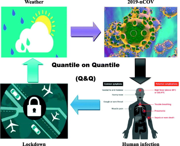
Graphical abstract
Highlights
-
•
Ø This paper examines the interlinkages between temperature and COVID-19 in the top ten coronavirus affected Chinese provinces.
-
•
Ø QQ approach of Sim and Zhou is applied to explore some nuanced features of temperature and COVID-19 nexus.
-
•
We find mostly positive relationship for Hubei, Hunan and Anhui between temperature and COVID-19.
-
•
Zhejiang and Shandong provinces are showing mostly negative impacts between temperature and COVID-19.
1. Introduction
Coronavirus is named after crown spikes have been found on its surface, and known species are 229E, NL63, OC43,HKU1, Severe Acute Respiratory Syndrome Coronavirus (SARS-CoV),1 and Middle East Respiratory Syndrome Coronavirus (MERS-CoV),2 where the latter two, originate from zoonotic diseases, associated with lethal diseases (Drosten et al., 2003; Zaki et al., 2012).
The World Health Organization (WHO) reported unknown cases of pneumonia in Wuhan, Hubei Province, China in December 2019 (Sohrabi et al., 2020; Zhu et al., 2020). Since the unexplained pneumonia was first reported on December 1, the COVID-19 pathogen was subsequently identified by the Chinese Center for Disease Control and Prevention (CDC) from the patient's pharyngeal swab samples and later named SARS-CoV-2 by WHO (Xi et al., 2020). Until January 7, 2020, China has reported that a serious corona viral acute respiratory syndrome coronavirus 2 (SARS-CoV-2) has been the cause of the epidemic of pneumonia (Li et al., 2020). SARS-CoV-2, the seventh human-infectious coronavirus, cases have developed rapidly in China (Lian et al., 2020).
Despite the great efforts of China, including the isolation of Wuhan City on 23 January, it spread rapidly, and 68,584 patients were infected by the 15 February of 2020. It spread all over the world because they did not know the intensity and emphasis of preventative and control measures. The top ten provinces in China affected by COVID-19 are shown in Fig. 1 .
Fig. 1.

Chinese top ten provinces affected by COVID-19.
Presently, the combat against COVID-19 is the most critical challenge for China, which has drawn international attention as well. Temperature and its changes have, according to records, affected the SARS outbreak (Lin et al., 2006). SARS-CoV Studies show that temperatures in the four major affected cities of Beijing and Guangzhou are significantly relate with the epidemic situation. Tan et al. (2005) found that the temperature was lower in the 2003 SARS outbreak and the risk of increased daily incidence maybe 18.18 times higher than that at high temperatures. Such studies have inspired us to conduct research on temperate and COVID-19.The temperature variation in the top ten COVID-19 affected provinces is shown in Fig. 2 .
Fig. 2.

Time trend of temperature (°C) of Chinese provinces.
In this study, a non-linear model containing the total number of accumulated confirmed cases and temperature is considered for the top ten most affected provinces of China with COVID-19. In the context of a novel quantile on quantile regression approach, this is the first analysis on Temperature and COVID-19. Herein, we also used this approach to test the multidirectional relation between temperature and COVID-19, somebody could argue about how COVID-19 can affect temperature. COVID-19 can have an indirect effect on temperature, for example, as a result of the coronavirus epidemic, the Chinese authorities are completely lock-down in China. Due to the complete lockdown, all manufacturing units were sealed, with less traffic flow (private and public transport, trains, airways) resulting in less carbon emissions. As the previous researcher suggested, there is a lower risk of ozone depletion due to lower carbon emissions (Papadimitriou, 2004). Less ozone depletion can therefore have an impact on daily temperatures. These arguments show that COVID-19 can have an indirect impact on temperature. Our main objective is to investigate the role of a particular meteorological variable in the spread of the COVID-19 epidemic.
2. Data and methodology
2.1. Data collection
For this study, ten most COVID-19 effected provinces of China were selected for the analysis. These provinces are Hubei, Guangdong, Henan, Zhejiang, Hunan, Anhui, Jiangxi, Shandong, Jiangsu, and Heilongjiang. COVID-19 data from January 22, 2020 to March 31, 2020 were obtained through the official website of China's National Health Commission. The daily temperature data for all the provinces were collected by Using WUC3 (Weather Underground Company). Herein, we collected temperature from capital city of each province. Because much of the population lives in the provincial capital city compared to others, and these cities often have main health facilities so that there is more patient presence in these cities than in others. Every capital city also has an International Airport. And in these areas the risks of the virus infection are higher (Leung et al., 2006). The map for our selected provinces is shown in Fig. 3 .
Fig. 3.

Sample based on Top 10 Chinese Provinces with maximum COVID-19 confirmed cases on 31, March 2020.
We have to check the normality of the data and the unit root test prior to using the QQR on the model of the study. The rationale of using the quantile-on-quantile method is to identify asymmetrical behavior between two given variables. Therefore, it is very robust to asymmetric distributions of non-normal data or variables (Shahbaz et al., 2018). The values of Jarque-Berra (JB) tests are mentioned in Table 1 . The JB findings are statistically significant at 1%, which indicates that the temperature distribution of the data and COVID-19 are asymmetric in all provinces. The non-normality of the variables also ensures that the QQR approach must be used.
Table 1.
Summary statistics and unit root tests.
| Provinces | N | Mean | Std. dev. | Min | Max | J-B Stats | ADF-1(1) | ZA-1(1) | Break day |
|---|---|---|---|---|---|---|---|---|---|
| COVID-19 | |||||||||
| Hubei | 70 | 968.586 | 2057.667 | 0 | 14,840 | 12.56*** | −5.266*** | −6.694*** | 19feb2020 |
| Guangdong | 70 | 21.343 | 28.813 | 0 | 99 | 30.11*** | −7.235*** | −4.835** | 09feb2020 |
| Henan | 70 | 18.229 | 28.461 | 0 | 109 | 27.83*** | −6.907*** | −4.978** | 09feb2020 |
| Zhejiang | 70 | 17.957 | 30.837 | 0 | 132 | 43.62*** | −7.062*** | −7.254*** | 09feb2020 |
| Hunan | 70 | 14.543 | 23.116 | 0 | 78 | 32.51*** | −7.554*** | −5.068** | 08feb2020 |
| Anhui | 70 | 14.143 | 22.19 | 0 | 74 | 24.53*** | −6.533*** | −5.185** | 11feb2020 |
| Jiangxi | 70 | 13.386 | 22.43 | 0 | 85 | 26.1*** | −5.952*** | −4.765* | 15feb2020 |
| Shandong | 70 | 11.057 | 26.02 | 0 | 203 | 11.87*** | −7.251*** | −9.092*** | 23feb2020 |
| Jiangsu | 70 | 9.229 | 13.174 | 0 | 39 | 23.62*** | −7.071*** | −6.351*** | 14feb2020 |
| Heilongjiang | 70 | 6.914 | 11.144 | 0 | 50 | 17.25*** | −4.741*** | −10.235*** | 08feb2020 |
| Temperature (°C) | |||||||||
| Hubei | 70 | 10.214 | 4.953 | 1 | 20 | 24.8*** | −7.763*** | −7.481*** | 21mar2020 |
| Guangdong | 70 | 18.329 | 4.069 | 8 | 25 | 10.67*** | −5.925*** | −6.290*** | 17feb2020 |
| Henan | 70 | 8.671 | 5.127 | −1 | 20.5 | 25.28*** | −9.264*** | −9.389*** | 21mar2020 |
| Zhejiang | 70 | 10.693 | 4.584 | 2.5 | 22 | 0.9329 | −7.066*** | −8.256*** | 21mar2020 |
| Hunan | 70 | 11.586 | 5.053 | 3 | 24 | 23.176*** | −7.743*** | −7.110*** | 21mar2020 |
| Anhui | 70 | 8.936 | 4.914 | −0.5 | 21 | 71.39*** | −7.581*** | −8.342*** | 21mar2020 |
| Jiangxi | 70 | 11.957 | 4.571 | 4.5 | 24 | 1.564 | −7.550*** | −7.703*** | 21mar2020 |
| Shandong | 70 | 7.95 | 5.532 | −3.5 | 19.5 | 18.74*** | −7.916*** | −7.445*** | 21mar2020 |
| Jiangsu | 70 | 9.543 | 4.593 | 1 | 21.5 | 26.77*** | −8.557*** | −8.106*** | 21mar2020 |
| Heilongjiang | 70 | −7.579 | 8.218 | −23 | 10 | 1.632 | −7.790*** | −7.827*** | 13feb2020 |
Note: *, **, *** indicates 1%, 5% and 10% level of significance; SD standard deviation; J-B is Jarque-Berra Normality Test
The unit root tests were also carried out to verify the data stationary of the selected variables. The findings of the Augmented Dickey-Fuller Analysis (AFD) indicate that all variables at levels are non-stationary. However, the ADF root test could lead to bias and misleading results if the data are non-normal or have structural break problems (Shahbaz et al., 2015). Following the empirical studies of Ahmed et al. (2019), a structural break test was used to determine the single structural break in data at a time (Zivot and Andrews, 2002). A significant advantage of the ZA unit root test is that it allows the determination of the break year to be carried out in an endogenous manner rather than on the basis of a prior set of information that mitigates the pre-testing problem. The unit root results of both ADF and ZA tests exhibit that both temperature and COVID-19 are non-stationary at level for all the provinces but become stationary at first difference. Therefore, both these variables are integrated of I (1) and have been converted into different series for QQR.
2.2. Quantile-on-Quantile Regression
The newly suggested QQ approach of Sim and Zhou (2015) explains the specification of following model. QQ approach is a more general form of standard quantile regression. This method allows for exploring the effect of quantile variables on other conditional quantile variables. This is the combination of quantile regression and non-parametric estimation. They used quantile regression to study the effect of one parameter of different quantiles of the dependent variable. This study shows the asymmetric relationship between temperature and COVID-19 in the top ten COVID-19 affected provinces in China. This approach gives details about how temperature quantities influence COVID-19 quantities, and gives more reliable and detailed information on the relation between the two variables.
Shahbaz et al. (2018) suggest that the QQR approach offers more comprehensive information and findings than ordinary lesser-quantiles and traditional quantile regression. They performed it in the following three steps. First, the effect of a specific quantile of temperature on COVID-19 has been evaluated by a local linear regression and vice-versa, to solve the problem of dimensionality by assigning further weights to values in the adjacent quantiles. Second, the classical quantile regression is applied to evaluate the effect of a predictor, say temperature, upon various quantiles of the criterion variable i.e., COVID-19. Third, the classical linear regression technique is also applied to test the impact of temperature upon COVID-19 at both tail and head quantiles of the data distribution and vice versa. Sharif et al. (2019) show that the QQR approach incorporates the properties of both non-parametric approach and quantile regression, and regress the temperature quantities to those of COVID-19 and vice versa to capture the model's asymmetric and spatial characteristics over time
In this study, the QQ method is suggested to use the variable quantiles to analyze the contribution of temperature by COVID-19 in the selected provinces. This method is based on a nonparametric quantile regression model.
| (1) |
where:
C194 t COVID-19 (Coronavirus Disease) of a province at period t,
Tempt Temperature (degree centigrade °C) in a province at given period t
∅ The ∅th quantile of the conditional distribution growth of C19,
ε t ∅ Quantile residual term whose conditional ∅th quantile is supposed to have zero value
β ∅(.) Known because no a priori information on interlinkages between C19 and Temp is available.
Quantile regression methods help to analyze the impact of temperature and COVID-19 at different quantiles in the top ten COVID-19 affected provinces in China. It is a very flexible technique because it can assess the functional dependence between C19 and Temp in the provinces. The key advantage of the specification is its flexibility as the functional relationship between C19 and Temp is not previously assumed. One major drawback with quantile regression techniques is that it does not differentiate how the varying levels of positive or negative Temp shocks affect COVID-19. Therefore, this study performed local linear regression to capture the asymmetric effect of Temp on C19. The expanded version of Eq. (1) using the Taylor method can be stated as follows:
| (2) |
Eq. (2) represents the application of local linear regression to capture the unique relation between the certain quantile of C19 (∅) and the certain quantile of Temp (T) in the immediate neighbor of Temp T .
Moreover, β ∅° measures the marginal effect of Temp by taking the partial differential of β ∅(Temp T) with respect to Temp of a certain province in ten provinces. The Eq. (2) represents dual indexing of quantile parameters, ∅ and T for C19 and Temp respectively. To capture the effect of quantiles of C19 on those of Temp, the Eq. (1) can be extended. Like Eq. (2), with the first order expansion method of Taylor to apply local linear regression in the neighborhood of C19T.
| (3) |
where δ ∅ represents of marginal effect of C19 in Eq. (2), and is the partial differential of δ ∅(C19T) with respect to C19. Moreover, both β ∅° and δ ∅° should be interpreted like the coefficients of traditional regression approach. In Eq. (2), β ∅(Temp T) and β ∅°(Temp T) can be represented:
| (4) |
where β 0(∅, T) and are the functional parameters of β ∅(Temp T)) and β ∅°(Temp T) depending upon the quantiles of ∅ and T. The similar functional forms can be derived for δ ∅(C19T) and δ ∅°(C19T) to determine the slope coefficients of C19 when Temp is dependent variable.
| (5) |
where, and represent the functional parameter of δ ∅(C19T) and δ ∅°(C19T) of local regression technique. If we replace the Eqs. (2), (3) into basic QQR equation then we can get following equations.
| (6) |
| (7) |
The part (∗) represents provisional conditional of ∅th quantile of C19 and Temp in Eqs. (6), (7). These formulas depict the true nexus between the quantiles of Temp and quantiles of C19 and vice versa due to double indexing of coefficients, in terms of ∅ and T, and this cross-dependence is also linked with their relative distributions. Finally, we provide estimated coefficients of Temp, as represented by β 0 and β 1, in Eq. (8) by applying local linear regression contingent upon minimization problem. Moreover, U⏜AGt and UAGτ ⏜ are the estimate.
| (8) |
The similar minimization problem can be derived for capturing the effect of COVID-19 on urban Temp in Eq. (9).
| (9) |
where, σ ∅(.) shows the quantile loss function and L (.) is the Gaussian kernel function in both the minimization problems as minimal weighting criterion to improve the estimation efficiency. The optimal bandwidth is necessary to ensure the balance between the estimation bias and the variation caused by higher or smaller interval of k. The selection of bandwidth, k, in this nonparametric QQR approach is very crucial as it determines the smoothness of the estimated coefficients. Based on previous studies we have selected 5% (h = 0.05) bandwidth of density function for optimal parameters of quantiles-on-quantiles approach (Arain et al., 2019; Sim and Zhou, 2015).
3. Results and discussions
3.1. Descriptive statistics and unit root
Summary statistics and unit root test for daily data pertaining to temperatures and COVID-19 for sampled provinces are given in Table 1. With an average value of 968.586, Hubei is the highest affected province COVID-19. As a mean value of more than 10, the provinces of Guangdong, Henan and Zhejiang are second, third, and fourth with mean values 21.343, 18.229 and 17.957 respectively. Heilongjiang has the lowest mean value as 6.914. As we examine the temperature data, it is find that Guangdong as the maximum mean value of 18.329 by following Jiangxi and Hunan 11.957, 11.586, respectively. For the unit root test and descriptive statistics see more details in Table 1.
The correlation between temperatures and COVID-19 for the coronavirus affected provinces is shown in Table 2 . From the correlation analysis, the highly negative correlation between temperatures and COVID-19 is well evident for, Guangdong, Henan, Jiangxi, Shandong and Jiangsu. While, for Hubei, Zhenjiang, Hunan, Anhui and Heilongjiang, COVID-19 and temperature are positively correlated.
Table 2.
Correlation analysis
| Country | Correlation | t-value | p-Value |
|---|---|---|---|
| Hubei | 0.5356257 | 5.2305 | 0.000 |
| Guangdong | −0.3038346 | 2.6298 | 0.010 |
| Henan | −0.5006191 | 4.7688 | 0.000 |
| Zhejiang | 0.4941642 | 4.6873 | 0.000 |
| Hunan | 0.4372964 | 4.0098 | 0.000 |
| Anhui | 0.5098245 | 4.8869 | 0.000 |
| Jiangxi | −0.5178269 | 4.9914 | 0.000 |
| Shandong | −0.5246733 | 5.0823 | 0.000 |
| Jiangsu | −0.5211593 | 5.0355 | 0.000 |
| Heilongjiang | 0.6612333 | 6.0262 | 0.000 |
3.2. Discussion Quantile-on-Quantile Regression (QQR)
In this study, the QQR method has been used to investigate the relationship between temperature and COVID-19 in case of coronavirus affected provinces in China. The QQR slope coefficients are shown in Fig. 4 representing the provinces-wise three-dimensional graphs in two columns. The first column captures the effect of τ th quantile of temperature on θ th equidistant quantile of COVID-19, as represented by β 1(θ,τ), for all ten provinces. Similarly, the second set of graphs in column 2 represents the slope parameters λ 1(θ,τ) measuring the effect of equidistant quantile τ th of COVID-19 on equidistant quantile θth of temperature. The graphical presentation of slope parameters of QQR estimation clearly indicates that the nexus between temperature and COVID-19 is not only symmetrical, but the shape of these quantile relational curves substantially varies across provinces and time periods.
Fig. 4.


Quantile on Quantile regression estimates slop of the coefficients,
In case of the Hubei province, there is a weak but positive impact of temperature on COVID-19 in the area of middle quantiles (0.4–0.5) of both variables, as revealed by Ma et al. (2020). In another surface of the graph, from quantiles (0.6–0.8) the negative effect of temperature on COVID-19 starts getting weaker, in the higher quantiles (0.7–0.9) of both variables, the impact is found insignificant in lower quantiles. Insignificant results also suggested by a recent study Iqbal et al. (2020) who studied wavelet coherent analysis on Wuhan dataset in the relationship between temperature and COVID-19. While on the other side, the influence of COVID-19 on temperature from the middle to higher quantiles (0.4–0.8) is found to be very weak and insignificant. However, we observe a very week negative impact of temperature on COVID-19 by combining both variables at lower quantiles (0.2–0.4). These segments of findings are in line with the finding of a recent paper (Tosepu et al., 2020). The Graph is also showing some negative and positive peaks for both variables which indicate the different trends in different Quantiles. In Guangdong province, there is a highly negative impact of temperature on COVID-19 in very initial quantile (0.05–0.2) for COVID-19 and same highly negative impact of temperature on COVID-19 from initial Quantiles to upper Quantiles (0.05–0.7). The graph shows that there is little positive impact of temperature on COVID-19 in middle Quantiles (0.4–0.6) for COVID-19 and also positive impact in lower Quantiles (0.2–0.4) for temperature. Results of higher Quantiles are showing insignificant results for both temperature and COVID-19. On the other hand, the impact of COVID-19 on temperature is showing minor negative impact in middle Quantiles (0.4–0.6) for temperature and impact is getting weaker from middle Quantiles to upper Quantiles (0.4–0.8) for COVID-19. Higher Quantiles for both Temperature and COVID-19 are showing positive impact.
In the case of Henan province, graph is showing insignificant in lower and upper Quantiles for COVID-19. There is only lower-middle Quantiles (0.3–0.4) showing a negative impact of temperature on COVID-19 for COVID-19. The Graph is also showing the strong positive impact of temperature on COVID-19 in initial Quantiles (0.0–0.4) for temperature, as recent study Ma et al. (2020) revealed that there are 2.92% COVID-19 deaths due to increase in one unit of temperature. On the other hand, the effect of COVID-19 on temperature is showing insignificant results in mostly Quantiles for both temperature and COVID-19 except the higher Quantiles (0.7–0.9), (0.7.5–0.8) for COVID-19 and temperature respectively. In the case of Zhenjiang province, there are showing the highly negative impact of temperature on COVID-19 in lower to middle Quantiles (0.0–0.4) for both variables. There is an only positive impact of temperature on COVID-19 monitored in the Quantiles (0.6–0.7) for COVID-19. All higher Quantiles (0.7–0.10) for both temperature and COVID-19 are showing completely significant results. Therefore the impact of COVID-19 on temperature is showing insignificant for all Quantiles for both temperature and COVID-19 except the last upper Quantiles.
In the case of Hunan province, a major part of the graph is showing the insignificant impact of temperature on COVID-19. There is a negative temperature effect on COVID-19 in Quantiles (0.5–0.7) for COVID-19 and lower Quantiles (0.1–0.4) for temperature. Only two peaks are showing the positive impact in upper Quantiles (0.75–0.8) for COVID-19. In the case of COVID-19, results are insignificant in lower Quantiles (0.1–0.2) and higher Quantiles (0.8–0.10). On the other hand, however, results show a slightly different picture of the middle quantiles (0.4–0.6) indicate that COVID-19 has a strongly negative effect on the temperature and getting lower and isignificant at the end. Initial quantiles (0.1–0.2) indicate insignificant results. The findings indicate a very different scenario in the case of Anhui as many peaks showed in graphs. For both COVID 19 and temperature there is only one pit which shows a negative relationship between temperature and COVID-19 in the upper quantiles. Lower Quantiles (0.1–0.2) indicate an increasingly positive trend for COVID-19. The overall graph shows insignificant results in higher quantiles. The impact of COVID-19 on temperature shows mixed results in different quantiles. Only higher quantiles (0.6–0.95) show a positive relationship between COVID-19 and temperature. There is an increasing trend from negative to insignificant in upper quantiles (0.6–0.95) of temperature.
There are also mixed negative and positive peaks in the graph in the case of Jiangxi Province that indicate different patterns. The graph reveals extremely negative temperature effect on COVID-19 from initial to middle COVID-19 quantiles (0.1–0.5) and decreasing temperature trend from negative to negligible found in all quantiles (0.1–1). For both variables, three peaks are also seen as a positive effect of temperature on COVID-19 in upper Quantiles. The impact of COVID-19 on the temperature variable is lower than that of COVID-19. The more region of the graph shows insignificant results for both variables. There is only one peak that indicates the negative effect of COVID-19 on the upper Quantile temperature (0.7–0.8). It usually indicates the very minimal temperature effect of COVID-19. In the case of Shandong Province, the quantiles (0.2–0.5) of COVID-19 have been monitored for a slightly negative impact to a very negative impact. From Quantiles Middle to Upper (0.5–0.9), findings at the top of Quantiles of (10) indicate insignificant trend to negative. The upper quantiles (0.6–0.9) show a positive to negative trend as the temperature impact on the COVID-19 temperature variable. The impact of COVID-19 on the temperature graph shows a very positive effect in lower quantiles (0.1–0.2) and a very negative effect in upper quantiles (0.8–10) respectively.
In the case of Jiangsu province, a major area of the graph is showing insignificant results except for some upward and downward peaks. In the middle Quantiles (0.4–0.6) there is a minor negative impact of temperature on COVID-19 for the variable of COVID-19. Some peaks in upper Quantiles (0.8–0.9) are showing a positive impact of temperature on COVID-19. There is also monitored the positive impact of temperature on COVID-19 at the upper Quantiles (0.8–10) of COVID-19. On the other hand, the graph shows totally insignificant results for both variables, as an effect of COVID-19 on temperature. Just one peak indicates the relative positive effect of COVID-19 on temperature in the 10th Temperature Quantiles. In Heilongjiang's case, the upper Quantiles (0.8–0.95) showed a positive temperature effect on COVID-19 in both variables with the increasing trend. There is only one v-shaped point, which for COVID-19 shows half negative impact to the upper quantiles and half positive to the lower quantiles. On the other hand, COVID-19 has a positive effect on the upper quantile temperature (0.8–0.9) and then has a positive effect in (10). There are insignificant results for the remaining graph.
3.3. Testing the validity of the QQ method
In the current analysis, the quantile-on-quantile method was applied to investigate the τth temperature quantile on θth quantile of COVID-19 and vice versa at different values of the respective quantiles. Therefore, this approach is more comprehensive to capture the asymmetric effect of temperature on COVID-19 across equidistant quantiles of τ and θ. However, the average values of slope parameters relating to QQR should be approximately similar to those of traditional quantile regression to validate the results of QQR approach in the previous discussion. In view of the decomposition characteristics inherent in the QQ method, the QQ estimate can be used to recover the estimate from the standard quantile regression. Specifically, the quantile regression parameter indexed only by θ can be generated by averaging the QQ parameter along τ. For example, the slope coefficient of the quantile regression model can be obtained by the following formula: This coefficient measures the impact of temperature on the distribution of COVID-19, which is expressed by γ1 (θ):
| (10) |
where is the number of quantiles and τ = [0.10, 0.15, …, 0.90] considered. Fig. 5 provides a comparative assessment of QQR with QR method; it confirms the previous findings and follows similar trends. The graphs of all provinces exhibit that the mean values of QQR coefficients is approximately parallel to those of QR coefficients and move along with each other. In some of the provinces like Henan, Jiangxi and Heilongjiang the trend in QQR line and QR line are alike, but the values are somewhat dissimilar. The graphical evidence postulates that the estimates from the quantile regression model can be recovered from the summary of detailed information available in QQ estimates. These findings authenticate our prior results of QQR approach in Fig. 4 .
Fig. 5.


Comparison between Quantile on Quantile and Quantile regression
4. Conclusion and policy implication
This research uses for the first time a comprehensive and latest methodology to examine the asymmetric nexus between temperature and COVID-19 in the top ten Chinese provinces affected by coronavirus (COVID-19) during the period from January 22, 2020 to March 31, 2020. Current study used the quantile (QQ) method of Sim and Zhou (2015) to confirm how each quantile of temperature affects each quantile of COVID-19, and therefore provides a new and complete description of the overall dependence of temperature and COVID-19 matched to the typical methodology, such as OLS or quantile regression. This approach also provides information as to how temperature quantities influence the COVID-19 quantities and gives more precisely and reliably knowledge about how these two variables interlink.
The empirical findings of this paper provide quite heterogeneous results across various syndicated areas formed by the quantiles of temperature and COVID-19; these results further very asymmetric behavior as predicted by QQR. The findings show that the temperature and COVID-19 relationship is found positive for Hubei, Hunan, and Anhui provinces of China as indicated by previous paper of Ma et al. (2020). Zhejiang and Shandong provinces are showing mostly negative relationship between temperature and COVID-19 as suggested by Tosepu et al. (2020). The remaining five provinces Guangdong, Henan, Jiangxi, Jiangsu, and Heilongjiang, are showing the mix trends as some lower Quantiles showing positive and upper Quantiles showing negative and vice versa. The variation trend between provinces in relation between temperature and COVID-19 can be explained by differences in the number of COVID-19 cases and the province's overall hospital facilitations. Temperature is also playing a very vital role in determining the epidemic situation in China, as suggested by our findings.
The findings also show that in different provinces of China it can be appropriate to maintain a stable and pleasant patient climate. Although the Quantiles on Quantiles analysis is relatively new and is better than the various correlations and many other time series techniques still require careful interpretation as the causality between temperature and COVID-19.
CRediT authorship contribution statement
Farrukh Shahzad: Writing - original draft, Conceptualization, Validation. Umer Shahzad: Supervision. Zeeshan Fareed: Data curation, Formal analysis, Methodology. Najaf Iqbal: Investigation, Data curation. Shujahat Haider Hashmi: Writing - review & editing. Fayyaz Ahmad: Writing - review & editing.
Declaration of competing interest
The authors declare that they have no known competing financial interests or personal relationships that could have appeared to influence the work reported in this paper.
Footnotes
In November 2002 SARS-CoV is diagnosed in Guangdong province of China. With the confirmed cases of 8096 observed mortality rate of around 10% of 744 patients. Symptoms were as same as recently diagnosed COVID-19 (Corona Virus). Male female affected ratio was monitored 1:1.25 (Wang et al., 2020)
In June 2012 MERS-CoV is diagnosed in Jeddah province of Saudi Arabia. With the confirmed cases of 2094 observed mortality rate of 37% of 858 patients. Symptoms were also same as recently diagnosed COVID-19(Corona virus). Male female affected ratio was monitored 3.3:1 (Wang et al., 2020)
We collected our weather variable (Temperature) data from this Website http://wunderground.com. Many previous papers have been used this website to collect weather data and paper have been published in high impact factor journals (Lu and Chou, 2012; Shahzad, 2019). So we can say this is authentic source to collect weather data.
In the Data and methodology section we used C19 as the abbreviation for COVID-19 because it was hard to write full name in equation.
Contributor Information
Farrukh Shahzad, Email: farrukh.hailian@gmail.com.
Zeeshan Fareed, Email: zeeshanfareed@hotmail.com.
References
- Ahmed Z., Wang Z., Ali S. Investigating the non-linear relationship between urbanization and CO 2 emissions: an empirical analysis. Air Qual. Atmos. Health. 2019;12(8):945–953. [Google Scholar]
- Arain H., Han L., Sharif A., Meo M.S. Investigating the effect of inbound tourism on FDI: the importance of quantile estimations. Tour. Econ. 2019;26(4):682–703. 1354816619859695. [Google Scholar]
- Drosten C., Günther S., Preiser W., Van Der Werf S., Brodt H.-R., Becker S., Fouchier R.A. Identification of a novel coronavirus in patients with severe acute respiratory syndrome. N. Engl. J. Med. 2003;348(20):1967–1976. doi: 10.1056/NEJMoa030747. [DOI] [PubMed] [Google Scholar]
- Iqbal N., Fareed Z., Shahzad F., He X., Shahzad U., Lina M. Nexus between COVID-19, temperature and exchange rate in Wuhan City: new findings from Partial and Multiple Wavelet Coherence. Sci. Total Environ. 2020;729 doi: 10.1016/j.scitotenv.2020.138916. [DOI] [PMC free article] [PubMed] [Google Scholar]
- Leung G., Lim W., Ho L.-M., Lam T.-H., Ghani A., Donnelly C.…Anderson R. Seroprevalence of IgG antibodies to SARS-coronavirus in asymptomatic or subclinical population groups. Epidemiol. Infect. 2006;134(2):211–221. doi: 10.1017/S0950268805004826. [DOI] [PMC free article] [PubMed] [Google Scholar]
- Li Q., Guan X., Wu P., Wang X., Zhou L., Tong Y., Wong J.Y. Early transmission dynamics in Wuhan, China, of novel coronavirus–infected pneumonia. N. Engl. J. Med. 2020;382(13):1199–1207. doi: 10.1056/NEJMoa2001316. [DOI] [PMC free article] [PubMed] [Google Scholar]
- Lian J., Jin X., Hao S., Cai H., Zhang S., Zheng L.…Zhang Y. Analysis of Epidemiological and Clinical features in older patients with Corona Virus Disease 2019 (COVID-19) out of Wuhan. Clinical Infectious Diseases. 2020 doi: 10.1093/cid/ciaa242. [DOI] [PMC free article] [PubMed] [Google Scholar]
- Lin K., Fong D.Y.-T., Zhu B., Karlberg J. Environmental factors on the SARS epidemic: air temperature, passage of time and multiplicative effect of hospital infection. Epidemiol. Infect. 2006;134(2):223–230. doi: 10.1017/S0950268805005054. [DOI] [PMC free article] [PubMed] [Google Scholar]
- Lu J., Chou R.K. Does the weather have impacts on returns and trading activities in order-driven stock markets? Evidence from China. J. Empir. Financ. 2012;19(1):79–93. [Google Scholar]
- Ma Y., Zhao Y., Liu J., He X., Wang B., Fu S.…Luo B. Effects of temperature variation and humidity on the death of COVID-19 in Wuhan, China. Science of The Total Environment. 2020;724 doi: 10.1016/j.scitotenv.2020.138226. [DOI] [PMC free article] [PubMed] [Google Scholar]
- Papadimitriou V. Prospective primary teachers' understanding of climate change, greenhouse effect, and ozone layer depletion. J. Sci. Educ. Technol. 2004;13(2):299–307. [Google Scholar]
- Shahbaz M., Solarin S.A., Sbia R., Bibi S. Does energy intensity contribute to CO2 emissions? A trivariate analysis in selected African countries. Ecol. Indic. 2015;50:215–224. [Google Scholar]
- Shahbaz M., Zakaria M., Shahzad S.J.H., Mahalik M.K. The energy consumption and economic growth nexus in top ten energy-consuming countries: fresh evidence from using the quantile-on-quantile approach. Energy Econ. 2018;71:282–301. [Google Scholar]
- Shahzad F. Does weather influence investor behavior, stock returns, and volatility? Evidence from the Greater China region. Phys. A Stat. Mech. Appl. 2019;523(C):525–543. [Google Scholar]
- Sharif A., Afshan S., Qureshi M.A. Idolization and ramification between globalization and ecological footprints: evidence from quantile-on-quantile approach. Environ. Sci. Pollut. Res. 2019;26(11):11191–11211. doi: 10.1007/s11356-019-04351-7. [DOI] [PubMed] [Google Scholar]
- Sim N., Zhou H. Oil prices, US stock return, and the dependence between their quantiles. J. Bank. Financ. 2015;55:1–8. [Google Scholar]
- Sohrabi C., Alsafi Z., O’Neill N., Khan M., Kerwan A., Al-Jabir A.…Agha R. World Health Organization declares global emergency: A review of the 2019 novel coronavirus (COVID-19) International Journal of Surgery. 2020;76:71–76. doi: 10.1016/j.ijsu.2020.02.034. [DOI] [PMC free article] [PubMed] [Google Scholar]
- Tan J., Mu L., Huang J., Yu S., Chen B., Yin J. An initial investigation of the association between the SARS outbreak and weather: with the view of the environmental temperature and its variation. J. Epidemiol. Community Health. 2005;59(3):186–192. doi: 10.1136/jech.2004.020180. [DOI] [PMC free article] [PubMed] [Google Scholar]
- Tosepu R., Gunawan J., Effendy D.S., Lestari H., Bahar H., Asfian P. Correlation between weather and Covid-19 pandemic in Jakarta, Indonesia. Sci. Total Environ. 2020;725 doi: 10.1016/j.scitotenv.2020.138436. [DOI] [PMC free article] [PubMed] [Google Scholar]
- Wang C., Horby P.W., Hayden F.G., Gao G.F. A novel coronavirus outbreak of global health concern. Lancet. 2020;395(10223):470–473. doi: 10.1016/S0140-6736(20)30185-9. [DOI] [PMC free article] [PubMed] [Google Scholar]
- Xi J., Xu K., Jiang P., Lian J., Hao S., Jia H.…Chen D. 2020. Virus strain of a mild COVID-19 patient in Hangzhou representing a new trend in SARS-CoV-2 evolution related to Furin cleavage site. medRxiv. [DOI] [PMC free article] [PubMed] [Google Scholar]
- Zaki A.M., Van Boheemen S., Bestebroer T.M., Osterhaus A.D., Fouchier R.A. Isolation of a novel coronavirus from a man with pneumonia in Saudi Arabia. N. Engl. J. Med. 2012;367(19):1814–1820. doi: 10.1056/NEJMoa1211721. [DOI] [PubMed] [Google Scholar]
- Zhu N., Zhang D., Wang W., Li X., Yang B., Song J.…Lu R. A novel coronavirus from patients with pneumonia in China, 2019. New England Journal of Medicine. 2020 doi: 10.1056/NEJMoa2001017. [DOI] [PMC free article] [PubMed] [Google Scholar]
- Zivot E., Andrews D.W.K. Further evidence on the great crash, the oil-price shock, and the unit-root hypothesis. J. Bus. Econ. Stat. 2002;20(1):25–44. [Google Scholar]