Does lockdown reduce air pollution? Evidence from 44 cities in northern China

Abstract

Responding to the ongoing novel coronavirus (agent of COVID-19) outbreak, China implemented “the largest quarantine in human history” in Wuhan on 23 January 2020. Similar quarantine measures were imposed on other Chinese cities within days. Human mobility and relevant production and consumption activities have since decreased significantly. As a likely side effect of this decrease, many regions have recorded significant reductions in air pollution. We employed daily air pollution data and Intracity Migration Index (IMI) data form Baidu between 1 January and 21 March 2020 for 44 cities in northern China to examine whether, how, and to what extent travel restrictions affected air quality. On the basis of this quantitative analysis, we reached the following conclusions: (1) The reduction of air pollution was strongly associated with travel restrictions during this pandemic—on average, the air quality index (AQI) decreased by 7.80%, and five air pollutants (i.e., SO₂, PM_2.5, PM₁₀, NO₂, and CO) decreased by 6.76%, 5.93%, 13.66%, 24.67%, and 4.58%, respectively. (2) Mechanism analysis illustrated that the lockdowns of 44 cities reduced human movements by 69.85%, and a reduction in the AQI, PM_2.5, and CO was partially mediated by human mobility, and SO₂, PM₁₀, and NO₂ were completely mediated. (3) Our findings highlight the importance of understanding the role of green production and consumption.

Graphical abstract

Highlights

• •We estimated the effects of the implementation of travel restrictions on air pollution.
• •We tested human mobility as one potential mechanism underlying this effect.
• •We utilized long dynamic panel data models using data from 44 cities in north China.
• •The concentrations of SO₂, PM_2.5, PM₁₀, NO₂, and CO decreased by 6.76%, 5.93%, 13.66%, 24.67%, and 4.58%, respectively.
• •Human mobility dropped by 69.85% after governments implemented travel bans.

1. Introduction

Beginning in December 2019 in Wuhan, Hubei Province, China, the ongoing outbreak of COVID-2019 spread rapidly across a wide range of countries, with the most affected countries being the United States, Spain, Italy, Germany, the United Kingdom, France, and China. As of 18 April 2020, a total of >2.3 million cases of COVID-2019 had been detected and confirmed in >200 countries and territories. To curb the dispersal of the disease from its source, a range of interventions, including travel restrictions, have since been implemented in various countries, which have been proven to be one of effective response measures in many countries(Paolo et al., 2011; Qi et al., 2016). In response to the pandemic, the Chinese central government imposed a lockdown in Wuhan, which has been referred to as the largest attempted cordon sanitaire in human history. The Wuhan lockdown set a precedent, and similar travel bans, including limits of nonessential movements in and out of cities, suspension of all transports, and closures of factories, were announced in other Chinese cities within days. These travel restrictions have since substantially mitigated the spread of COVID-2019 (Chinazzi et al., 2020; Kraemer et al., 2020; Tian et al., 2020).

As a possible side effect of this unprecedented lockdown, many regions experienced a dramatic reduction in air pollution. In China, Finland's Centre for Research on Energy and Clean Air reported that measures to contain the spread of COVID-19, such as travel restrictions and factory closures, produced a 25% drop in CO₂ (Carbon Brief 2020, https://www.carbonbrief.org). Similarly, the European Space Agency (ESA) satellite imagery showed a significant decline in NO₂ emissions in northern Italy between 1 January and 11 March 2020, coinciding with lockdowns to combat coronavirus. Additionally, the Institute of Environmental Science and Meteorology (IESM) estimated that since the implementation of the Luzon enhanced community quarantine on 16 March 2020, Metro Manila's PM_2.5 and PM₁₀ emissions were reduced significantly as a result of decreased utilization of machines that crush and grind as well as low dust exposure from roads. Wang et al. (2020) empirically found that anthropogenic emission decreases due to suspension of transportation and industry, contributed to the decreases of PM_2.5 concentrations.

Human health is strongly influenced by air quality. According to the 2019 State of Global Air Report, air pollution killed an estimated 5 million people globally in 2017, and China topped the 10 countries with the highest mortality (1.2 million) (Health Effects Institute, see https://www.healtheffects.org/). Massive research conducted over the past several decades has revealed that air pollution causes people to die younger as a result of cardiovascular (Peng et al., 2009; Wong et al., 1999) and respiratory diseases (Katanoda et al., 2011; Nakao et al., 2018; Spix et al., 1998). A recent study conducted by Zhu et al. (2020) suggested that there is a relationship between higher concentrations of air pollutants and higher risk of COVID-19 infection.

As one of the most populous countries and one in which air pollution exposure historically has been among the highest globally, in recent years, China has begun to move aggressively to reduce air pollution. China's air pollution is still worse than that experienced, on average, around the globe, especially in northern China (Chen et al., 2017; Yao et al., 2016). According to the most recent data of the Ministry of Ecology and Environment (MEE) of China, February 2020, the top 10 cities with the poorest air quality were Yuncheng, Taiyuan, Baotou, Shijiazhuang, Linfen, Tangshan, Urumqi, Xianyang, Weinan, and Baoding, all of which are located in northern China.

Many air pollution studies have illuminated that human-related activities, such as industrial production (Cole et al., 2005), traffic, and transportation (Chen et al., 2017; Fu and Gu, 2017; Lin Lawell et al., 2011), are the major contributors to air pollution, and extreme measures of full or partial lockdown may bring these production and consumption activities almost to a standstill. This context provides us with a unique opportunity to examine the effects of human-related activities on air quality. Although satellite data have offered suggestive evidence of significant drops in air pollution concentration during lockdowns, it is insufficient to understand the pollution reduction effects of the unprecedented quarantine resulting from the COVID-19 outbreak. Questions remain as to whether, how, and to what extent these interventions affected air quality. Instead, this work employs daily air pollution data (including air quality index [AQI], SO₂, PM_2.5, PM₁₀, NO₂, and CO), daily weather data, real-time human mobility data, and lockdown time lines of 44 cities in north China from a span of 1 January and 21 March 2020 (covered 81 days) to estimate the effects of travel restrictions on air pollutants concentration. Particularly, we first employ Least Square Dummy Variable (LSDV) estimation strategies to examine the effect of lockdown measures on air pollution. We find that, on average, the AQI reduced by 7.80%, and the concentration of five air pollutants (SO₂, PM_2.5, PM₁₀, NO₂, and CO) reduced by 6.76%, 5.93%, 13.66%, 24.67%, and 4.58%, respectively, after the implementation of lockdowns. We also estimate the mediating effect of human mobility, measured by IMI index from Baidu, on the relationship between the lockdowns and air pollution. We discover that travel restrictions lead a reduction of human mobility by 69.85%, and SO₂, PM₁₀, and NO₂ are fully mediated by human mobility and 44.9%, 9.3%, and 16.2% of the variations in AQI, PM2.5, and CO could be attributed to variations in human mobility, respectively.

This study has six sections. Section 2 introduces materials and data. Section 3 presents the specification of econometric model. Section 4 provides the basic empirical results. Section 5 offers a further research of mechanism and provides an analysis. Section 6 concludes.

2. Materials and data

2.1. Study area

Considering the fact that northern China has suffered from long-term air pollution and that the average concentration of air pollutants is much higher in the north than in other regions, we confined the study area to 44 cities in the Jing-jin-ji metropolitan circle and its surrounding areas. These 44 cities were included in the Program for Air Pollution Control and Supervision during the autumn and winter in the Jing-jin-ji Region and Surrounding Areas issued by the MEE in 2018, which officially set specific environmental performance goals for these 44 cities (Songke et al., 2014) (Fig. 1 ).

Fig. 1.

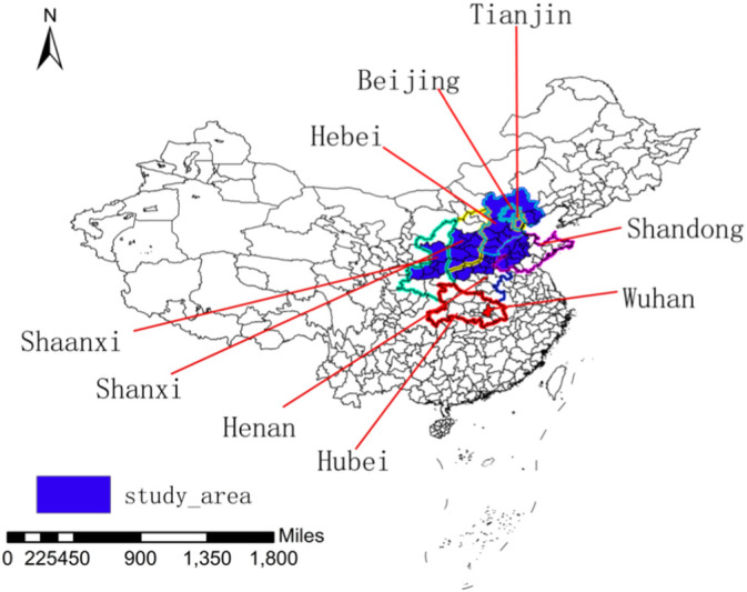
Study area.

According to the latest data from the China City Statistical Yearbook (2018). The population living in these 44 cities accounted for 19.25% of the total, whereas the percentage of land area was only 9.5% of mainland China. As one of the most economically developed regions, 20.86% of gross domestic product (current prices) and 16.33% of industrial enterprises are concentrated here. We also computed the number of buses and trolley buses (1,233,289) and taxis (232,742) under operation, which accounted for 21.91% and 25.76% of the total, respectively. Note, however, that the emission of industrial “three wastes” in these 44 cities, including SO₂, NO₂, and PM_2.5, as well as soot and dust, accounted for 22.43%, 24.59%, 21.18%, and 22.59% of the total, respectively. Therefore, we considered these 44 cities as our study area.

2.2. Data and variables

The two main data sets used in our baseline regression were (1) the daily air pollution data and (2) the daily weather conditions data for 44 cities.

2.2.1. Dependent variable: Air pollution

AQI and six pollutants (SO₂, NO₂, PM₁₀, PM_2.5, CO, and O₃) are commonly used to evaluate air quality (Xiao et al., 2018). In this study, we collected 24-h daily data of AQI, PM₁₀, SO₂, NO₂, PM_2.5, and CO data for 44 cities between 1 January and 21 March 2020 from the real-time monitoring data system of the MEE (http://datacenter.mee.gov.cn/). Furthermore, we calculated the daily average (i.e., arithmetic mean of a 24-h monitoring value on a natural day) of these data as the proxy for the explained variable (air pollution).

2.2.2. Independent variable: Lockdown

As part of the emergency response to the growing pandemic of COVID-2019, the Chinese government launched a radical lockdown campaign to prevent the spread of the virus. In what has been described as “the people's war,” the “Wuhan lockdown” was first implemented on 23 January 2020. Within days of the Wuhan lockdown, travel restrictions were imposed on other Chinese cities. For example, on 28 January 2020, a quarantine marked by the suspension of bus service was announced in Beijing, the capital city of China. As of 12 February 2020, at least 207 cities in China (including 26 provincial capitals and sub-provincial cities) announced travel bans. Travel restrictions inevitably altered the proportion of human-related production and consumption activities. This context provided a unique opportunity to systematically study whether and to what extent travel restriction measures shaped air quality. In particular, we coded a binary variable, which captured travel restrictions in 44 cities, as 1 if a city government adopted a quarantine policy and as 0 otherwise. Fig. 2 illustrates the detailed shutdown timeline for these 44 cities.

Fig. 2.

Dates of discovery of COVID-2019, and lockdown timeline of cities in Hubei Province and 44 cities in northern China beginning 31 December 2019.

2.2.3. Control variable: Weather conditions

Weather conditions influence the formation and diffusion of air pollutants (Kallos et al., 1993; Yen et al., 2013). We downloaded city-level weather conditions data (see https://freemeteo.cn/weather), which contained daily maximum and minimum temperatures, daily maximum wind and gust speeds, and records of rain and snowfall. These meteorological factors are closely related to air pollution. Considering that low temperature may be beneficial to improve air quality, we computed the daily mean temperature and its first differenced values (i.e., D. meantem) as the control variable in our regression equation.

Table 1 reports the variable definitions and descriptive statistics for these variables. As shown in the table, pollutant concentrations under lockdown were apparently higher than on those in regular days. For example, average PM_2.5 concentration was 76.110 μg/m³ with an average level of 65.811 μg/m³ during the lockdown periods and 81.363 μg/m³ on regular days, respectively, both of which exceeded World Health Organization (WHO) guideline and even WHO's least-stringent target (35 μg/m³). Other pollutants showed similar characteristics. Additionally, across the 44 cities, travel was restricted for 1204 days.

Table 1.

Descriptive statistics.

Variable category	Variable definition	Full sample		Lockdowns		Regular days		Std. Dev.	Min	Max
		Obs.	Mean	Obs.	Mean	Obs.	Mean
Explained variable: Air pollutants
AQI	Daily air quality index	3564	107.376	1204	92.645	2360	114.891	59.792	21.083	416.208
SO2	Daily SO2 concentrations (μg/m3)	3564	15.148	1204	13.835	2360	15.818	10.600	1.833	142.667
PM2.5	Daily PM2.5 concentrations (μg/m3)	3564	76.110	1204	65.811	2360	81.363	52.772	3.875	384.208
PM10	Daily PM10 concentrations (μg/m3)	3564	107.601	1204	85.811	2360	118.717	59.220	8.542	455.667
NO2	Daily NO2 concentrations (μg/m3)	3564	35.077	1204	23.640	2360	40.911	17.695	2.875	110.458
CO	Daily CO concentrations (mg/m3)	3564	1.144	1204	1.020	2360	1.207	0.607	0.185	7.417
Explanatory variable: Lockdown dummy
Lockdown	Lockdown dummy	3564	0.338	1204	1.000	2360	0.000	0.473	0.000	1.000
Control variable: Weather conditions
Hightem	Daily maximum temperature (°C)	3564	−2.159	1204	−3.535	2360	−1.456	4.728	−18.000	13.000
Lowtem	Daily minimum temperature (°C)	3564	10.373	1204	9.806	2360	10.661	6.528	−4.000	29.000
Meantem	Daily average temperature (°C)	3564	4.107	1204	3.136	2360	4.603	5.192	−10.000	19.500
Maxwind	Daily maximum steady wind (Km/h)	3564	18.363	1204	18.273	2360	18.409	8.396	7.000	68.000
Maxgust	Daily maximum gust (Km/h)	3564	25.032	1204	24.811	2360	25.466	13.911	7.000	101.000
Rain	Rain dummy	3564	0.106	1204	0.100	2360	0.120	0.308	0.000	1.000
Snow	Snow dummy	3564	0.034	1204	0.028	2360	0.047	0.182	0.000	1.000

3. Method of analysis

3.1. Baseline regression

Given that the baseline model included lagged values of the dependent variable, we estimated a city dynamic panel data model. The model can be presented as follows:

$${\mathit{\text{Ln(Air}}}_{i\mathit{,}t}\mathit{\text{)}}=\sum _{s=1}^{\mathrm{p}}{\rho }_{s}Ln\left(Ai{r}_{i\mathit{,}t\mathit{-}s}\right)+\beta ·L{\mathit{\text{ockdown}}}_{i\mathit{,}t}+\lambda \mathit{·}C{V}_{i,t}+f\left(t\right)+{\upsilon }_i+{\epsilon }_{i,t},$$ ₍₁₎

where the dependent variable Ln(Air_i,t) is the air quality index (AQI) and one of five air pollutants in city i on day t (i.e., logarithm of AQI, SO₂, PM_2.5, PM₁₀, NO₂, or CO), i = 1, …, 44 indexes 44 cities in north China, t = 1 January 2020, …, 21 March 2020 index dates (81 days); and lnair _i,t, as one of the regressors, is a lagged dependent variable. We used a general-to-specific sequential t rule and AIC/BIC methods to determine the optimal lag length p; lockdown _i,t is a dummy variable set to 1 if a day is among one of the lockdown days; CV _i,t is a set of control variables; f(t) is a time trend term controlling for inertial trends that may affect daily air quality; ν _i is city fixed effects; ε _i,t is a stochastic error term; and ρ, β, and λ are the parameters to be estimated.

Differences in the generalized method of moments (GMMs) and system GMM are two popular approaches used to estimate a dynamic fixed effects model, which includes lagged dependent variables. These two methods, however, are applicable only in a short panel model in which n is large and T is small. In this study, we used a longer, narrower panel with n = 44 and T = 81. For a long panel data model that does not include exogenous explanatory variables, the bias approaches 0 as T approaches infinity. Thus, we considered the Least Square Dummy Variable (LSDV) model estimator to be an appropriate empirical strategy for our study.

3.2. Testing the mechanism

Even though we established a link between the initial variable (travel restrictions) and an outcome variable (air pollution emission) in Eq. (1), the mechanisms underlying this relationship remained in question. We turned our attention toward understanding one potential mechanism—that is, human mobility. To mitigate the further dispersal of COVID-19, unprecedented interventions were undertaken. Human mobility within cities was substantially reduced in combination with travel restrictions in and out of cities, all of the public transport was suspended, and factories and schools were closed. Therefore, we considered human mobility as the mediator. More specifically, we tested the human mobility impact according to the following three steps.

First, we established the correlation between the initial variable (lockdowns) and the mediator (human mobility) using the mediator as a criterion variable in a regression equation and the initial variable as a predictor. We estimate the following model:

$$Ln\left(Human\mathit{\_}mobilit{y}_{i,t}\right)=\alpha +\beta ·Lockdow{n}_{i,t}+\lambda ·C{V}_{i,t}+{\nu }_i+{\epsilon }_{i,t}$$ (2)

where human_mobility _i,t denotes the degree of human movements measured by the Intracity Migration Index (IMI) in city i at day t. Other variables have the same implications as given in the Eq. (1).

Second, we correlated the mediator with the outcome variable (air pollution). To be specific, we used air pollutants emission as the criterion variable in a regression equation and human mobility as the predictors. The equation is specified as follows:

$${\mathit{\text{Ln(Air}}}_{i\mathit{,}t}\mathit{\text{)}}=\sum _{s=1}^{\mathrm{p}}{\rho }_{s}Ln\left(Ai{r}_{i,t-s}\right)+\beta ·H\mathit{\text{uman}}\mathit{\_}{\mathit{\text{mobility}}}_{i\mathit{,}t}+\lambda \mathit{·}C{V}_{i,t}+f\left(t\right)+{\upsilon }_i+{\epsilon }_{i,t}$$ (3)

where variables and parameter without specific interpretation are equal to those introduced in Eqs. (1), (2).

Third, it was not sufficient just to correlate the mediator with the outcome. The mediator (human mobility) and outcome variable (air pollution) may be correlated because they both were caused by the travel restriction. The effect of travel restrictions on air pollution controlling for mediator should be estimated as shown in the following regression equation:

$$\begin{array}{ccc}& & \\ Ln\left(Ai{r}_{i\mathit{,}t}\right)& \mathit{=}& {\sum }_{s=1}^{\mathrm{p}}{\rho }_{s}Ln\left(Ai{r}_{i,t-s}\right)\mathit{+}{\beta }_1\mathit{·}{\mathit{\text{Lockdown}}}_{i\mathit{,}t}\mathit{+}{\beta }_2\mathit{·}\mathit{\text{Human}}\mathit{\_}{\mathit{\text{mobility}}}_{i\mathit{,}t}\\ & & \mathit{+}\lambda \mathit{·}C{V}_{i\mathit{,}t}\mathit{+}f\left(t\right)\mathit{+}{\upsilon }_i\mathit{+}{\epsilon }_{i\mathit{,}t}\end{array}$$ (4)

where variables and parameters have the same meaning as given for Eqs. (1), (2).

4. Empirical results

4.1. Graphic analysis

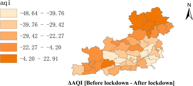
As a visual demonstration of the air pollution variation, we first employed a map tool in ArcGIS 10.2 to graphically depict the distribution of pollutants concentrations (see Fig. 3 ). This was done by comparing each city's air pollutants emissions before and after the lockdowns. As illustrated in Fig. 3, the spatial-temporal distribution of different air pollutants was significantly heterogeneous among cities. Specifically, the concentrations of five air pollutants during the lockdowns appeared to be much lower than concentrations on regular days, which offered supportive evidence of the pollution reduction effects of travel restrictions. In the following subsections, we further modeled the effects given by the Eq. (1).

Fig. 3.

Variations of AQI index, SO₂, PM_2.5, PM₁₀, NO₂, and CO concentrations before and after lockdowns.

4.2. Benchmark regression results

Table 2 reports the overall LSDV regression by estimating the extent to which lockdown predicted reductions of air pollution. The dependent variables are the logarithm of AQI, SO₂, PM_2.5, PM₁₀, NO₂, and CO. All control variables are included in the six models. Additionally, we included time trend terms and city fixed effects to account for temporal and regional variations.

Table 2.

Baseline regression for full samples.

Variables	(1) Ln(AQI)	(2) Ln(SO2)	(3) Ln(PM2.5)	(4) Ln(PM10)	(5) Ln(NO2)	(6) Ln(CO)
Lockdown	−0.0780⁎⁎⁎ (−6.0266)	−0.0676⁎⁎⁎ (−6.0003)	−0.0593⁎⁎⁎ (−4.1475)	−0.1366⁎⁎⁎ (−10.2586)	−0.2467⁎⁎⁎ (−13.8099)	−0.0458⁎⁎⁎ (−3.3007)
Lowtem	0.0134⁎⁎⁎ (4.9654)	−0.0113⁎⁎⁎ (−4.2123)	0.0161⁎⁎⁎ (5.1485)	0.0113⁎⁎⁎ (3.8673)	−0.0054⁎ (−1.9692)	0.0102⁎⁎⁎ (4.3940)
Hightem	0.0096⁎⁎⁎ (5.4290)	0.0268⁎⁎⁎ (8.5394)	0.0067⁎⁎⁎ (3.0368)	0.0175⁎⁎⁎ (7.9743)	0.0173⁎⁎⁎ (9.8751)	0.0074⁎⁎⁎ (4.4136)
D. meantem	0.0207⁎⁎⁎ (5.2470)	0.0155⁎⁎⁎ (3.7546)	0.0320⁎⁎⁎ (5.7489)	0.0229⁎⁎⁎ (5.7645)	0.0239⁎⁎⁎ (5.6181)	0.0160⁎⁎⁎ (3.7053)
Maxwind	−0.0022 (−1.5579)	−0.0006 (−0.3758)	−0.0012 (−0.6222)	−0.0024 (−1.4255)	−0.0008 (−0.3962)	0.0012 (0.6670)
Maxgust	−0.0063⁎⁎⁎ (−6.3484)	−0.0062⁎⁎⁎ (−4.9933)	−0.0124⁎⁎⁎ (−10.6413)	−0.0062⁎⁎⁎ (−5.0850)	−0.0087⁎⁎⁎ (−7.8728)	−0.0086⁎⁎⁎ (−7.6721)
Rain	0.0054 (0.2743)	−0.0912⁎⁎⁎ (−3.2911)	0.0508⁎ (1.8673)	−0.0214 (−0.9028)	0.0131 (0.6053)	0.0606⁎⁎⁎ (4.3119)
Snow	−0.0914⁎⁎⁎ (−3.7358)	−0.0482 (−1.2432)	−0.1193⁎⁎⁎ (−3.4968)	−0.1686⁎⁎⁎ (−6.4629)	0.0261 (0.8012)	0.0101 (0.3582)
Timetrend	−0.0075⁎⁎⁎ (−10.7262)	−0.0065⁎⁎⁎ (−7.5435)	−0.0101⁎⁎⁎ (−12.8593)	−0.0072⁎⁎⁎ (−8.4292)	−0.0036⁎⁎⁎ (−6.8208)	−0.0094⁎⁎⁎ (−11.9917)
Lag length (p)	2	3	4	4	3	4
City fixed effects	Yes	Yes	Yes	Yes	Yes	Yes
Constants	2.8751⁎⁎⁎ (32.8429)	1.3936⁎⁎⁎ (16.4894)	3.1002⁎⁎⁎ (37.2285)	2.8735⁎⁎⁎ (31.1057)	1.7736⁎⁎⁎ (14.4715)	0.4806⁎⁎⁎ (19.0019)
Sample size	3476	3432	3388	3388	3432	3388
R2	0.6218	0.6721	0.6514	0.5832	0.6895	0.6655

Note: t statistics in parentheses, standard errors are clustered at city level (44 clusters). ^⁎p < .10 indicates significance at 10% levels. ^⁎⁎⁎p < .01 indicates significance at 1% levels.

The results showed that lockdown negatively and significantly predicted a decrease in air pollution. In particular, AQI decreased by 7.80% during the lockdown compared with a regular day. The concentrations of the other five air pollutants (SO₂, PM_2.5, PM₁₀, NO₂, and CO) decreased by 6.76%, 5.93%, 13.66%, 24.67%, and 4.58%, respectively. The results given in Table 2 suggest that the implementation of travel restrictions dramatically reduced air pollution in 44 cities in northern China. Additionally, however, we found that the reduction ratio largely varied among the different air pollutants. Among them, PM₁₀ and NO₂ showed a higher reduction ratio. This largely was due to the pollution source of different pollutants. PM₁₀ and NO₂ resulted primarily from vehicle exhaust and road dust generated by transportation.

In the overall model, weather condition variables are signed as expected except maxwind. We noticed that lowtem had heterogeneous impacts on air pollution, which had a significantly negative correlation with SO₂ and NO₂, but had a positive relationship with AQI, PM_2.5, PM₁₀, and CO. The coefficients Hightem and D. meantem were positively significant (P < .01), indicating that air pollution may have increased as the temperature rose, which was to be expected. We additionally observed that maxgust helped reduce the concentration of air pollutants.

4.3. Robustness check

4.3.1. City-specific time trends

Considering that each city's ability to prevent pollution may be different, we estimated an individual fixed effects regression by modeling city-specific trends as a robustness check. The model considered the following:

$$\mathit{\text{Ln}}\left(Ai{r}_{i\mathit{,}t}\right)=\sum _{s=1}^{\mathrm{p}}{\rho }_{s}Ln\left(Ai{r}_{i\mathit{,}t\mathit{-}s}\right)+\beta ·{\mathit{\text{Lockdown}}}_{i,t}+\lambda \mathit{·}C{V}_{i,t}+f_i\left(t\right)+{\upsilon }_i+{\epsilon }_{i,t}$$ (5)

where f _i (t) indicates an individual time trends for city i, and other variables have the same meanings as in Eq. (1). The estimated results are shown in Table 4 and are consistent with Table 3 results.

Table 4.

Robustness check II: LSDV estimators for a shorter panel sizes (T = 61).

Variables	(1) Ln(AQI)	(2) Ln(SO2)	(3) Ln(PM2.5)	(4) Ln(PM10)	(5) Ln(NO2)	(6) Ln(CO)
Lockdown	−0.0975⁎⁎⁎ (−6.5822)	−0.0622⁎⁎⁎ (−4.7698)	−0.1226⁎⁎⁎ (−7.4392)	−0.1684⁎⁎⁎ (−11.8536)	−0.2227⁎⁎⁎ (−11.2746)	−0.0732⁎⁎⁎ (−5.3935)
Lowtem	0.0253⁎⁎⁎ (6.7461)	−0.0073⁎ (−1.9485)	0.0299⁎⁎⁎ (6.6746)	0.0234⁎⁎⁎ (5.4291)	−0.0050 (−1.4441)	0.0171⁎⁎⁎ (5.3057)
Hightem	0.0079⁎⁎⁎ (3.8081)	0.0247⁎⁎⁎ (7.5213)	0.0099⁎⁎⁎ (3.6018)	0.0153⁎⁎⁎ (6.0013)	0.0141⁎⁎⁎ (5.3897)	0.0090⁎⁎⁎ (4.3871)
D.meantem	0.0235⁎⁎⁎ (4.9696)	0.0162⁎⁎⁎ (3.3876)	0.0291⁎⁎⁎ (4.8843)	0.0242⁎⁎⁎ (5.4479)	0.0274⁎⁎⁎ (5.4372)	0.0132⁎⁎ (2.5963)
Maxwind	−0.0003 (−0.1458)	−0.0022 (−1.0573)	−0.0015 (−0.7010)	−0.0000 (−0.0144)	−0.0034 (−1.6005)	0.0005 (0.2576)
Maxgust	−0.0096⁎⁎⁎ (−8.1443)	−0.0064⁎⁎⁎ (−4.2585)	−0.0136⁎⁎⁎ (−9.7605)	−0.0091⁎⁎⁎ (−5.9308)	−0.0090⁎⁎⁎ (−6.7779)	−0.0093⁎⁎⁎ (−6.6697)
Rain	0.0201 (0.8590)	−0.0909⁎⁎⁎ (−2.8284)	0.0549 (1.6144)	0.0002 (0.0063)	−0.0017 (−0.0684)	0.0426⁎⁎ (2.2963)
Rnow	−0.1024⁎⁎⁎ (−4.6398)	−0.0255 (−0.7407)	−0.1200⁎⁎⁎ (−3.3201)	−0.1684⁎⁎⁎ (−7.2481)	−0.0631 (−1.5299)	0.0011 (0.0301)
Lag length (p)	2	3	4	4	3	4
Individual fixed effects	Yes	Yes	Yes	Yes	Yes	Yes
Constants	3.2971⁎⁎⁎ (33.5944)	1.7886⁎⁎⁎ (17.9658)	3.8237⁎⁎⁎ (37.2185)	3.5374⁎⁎⁎ (27.3138)	1.8943⁎⁎⁎ (12.9184)	0.6322⁎⁎⁎ (20.8032)
Sample size	2596	2552	2508	2508	2552	2508
R2	0.6303	0.6945	0.6481	0.6204	0.6796	0.6256

Note: t statistics in parentheses, standard errors are clustered at city level (44 clusters) ^⁎p < .10, indicate significance at 10% levels. ^⁎⁎p < .05, indicate significance at 5% levels. ^⁎⁎⁎p < .01 indicate significance at 1% levels.

Table 3.

Robustness check I: LSDV estimators including city-specific time trends.

Variables	(1) Ln(AQI)	(2) Ln(SO2)	(3) Ln(PM2.5)	(4) Ln(PM10)	(5) Ln(NO2)	(6) Ln(CO)
Lockdown	−0.0810⁎⁎⁎ (−6.0455)	−0.0608⁎⁎⁎ (−4.8459)	−0.0662⁎⁎⁎ (−4.2961)	−0.1417⁎⁎⁎ (−9.5836)	−0.2593⁎⁎⁎ (−13.8473)	−0.0512⁎⁎⁎ (−3.4102)
Lowtem	0.0145⁎⁎⁎ (5.2624)	−0.0081⁎⁎⁎ (−3.1190)	0.0155⁎⁎⁎ (4.6768)	0.0143⁎⁎⁎ (5.2147)	−0.0046 (−1.6216)	0.0101⁎⁎⁎ (4.6674)
Hightem	0.0123⁎⁎⁎ (6.3449)	0.0309⁎⁎⁎ (9.4668)	0.0093⁎⁎⁎ (3.7508)	0.0210⁎⁎⁎ (9.2286)	0.0181⁎⁎⁎ (9.5330)	0.0093⁎⁎⁎ (4.8992)
D. meantem	0.0176⁎⁎⁎ (4.4090)	0.0108⁎⁎ (2.6466)	0.0295⁎⁎⁎ (5.3926)	0.0187⁎⁎⁎ (4.4870)	0.0228⁎⁎⁎ (5.2752)	0.0137⁎⁎⁎ (3.1866)
Maxwind	−0.0026⁎ (−1.7713)	−0.0001 (−0.0637)	−0.0018 (−0.9018)	−0.0025 (−1.4845)	−0.0005 (−0.2719)	0.0011 (0.6189)
Maxgust	−0.0062⁎⁎⁎ (−6.2726)	−0.0064⁎⁎⁎ (−5.2969)	−0.0122⁎⁎⁎ (−10.5979)	−0.0060⁎⁎⁎ (−4.8244)	−0.0088⁎⁎⁎ (−7.7190)	−0.0087⁎⁎⁎ (−7.4148)
Rain	0.0112 (0.5656)	−0.0843⁎⁎⁎ (−3.0864)	0.0584⁎⁎ (2.1616)	−0.0153 (−0.6502)	0.0162 (0.7381)	0.0679⁎⁎⁎ (4.8762)
Rnow	−0.0889⁎⁎⁎ (−3.7403)	−0.0586 (−1.5370)	−0.1199⁎⁎⁎ (−3.7414)	−0.1718⁎⁎⁎ (−7.0825)	0.0258 (0.7746)	0.0165 (0.5609)
Lag length (p)	2	3	4	4	3	4
Individual fixed effects	Yes	Yes	Yes	Yes	Yes	Yes
Individual time trend	Yes	Yes	Yes	Yes	Yes	Yes
Constants	3.0611⁎⁎⁎ (35.2594)	1.4829⁎⁎⁎ (19.0725)	3.3092⁎⁎⁎ (41.1054)	3.0234⁎⁎⁎ (32.5320)	1.7711⁎⁎⁎ (14.7343)	0.5196⁎⁎⁎ (23.0206)
Sample size	3476	3432	3388	3388	3432	3388
R2	0.6306	0.6836	0.6576	0.5923	0.6926	0.6756

Note: t statistics in parentheses, standard errors are clustered at city level (44 clusters) ^⁎p < .10, indicate significance at 10% levels. ^⁎⁎p < .05, indicate significance at 5% levels. ^⁎⁎⁎p < .01, indicate significance at 1% levels.

4.3.2. A shorter panel size

To ensure that empirical results were robust, we turned our attention to address potential bias of the LSDV estimators for various panel sizes (i.e., whether the previous results were sensitive to the window width before and after the lockdowns) by changing the window width. Specifically, we dropped the observations of cities at the head (1–10 January) and the tail (12–21 March) separately. On the basis of the limited samples between 11 January and 11 March 2020, we re-estimated our model. The results are given in Table 4 . These results were similar to our earlier benchmark finding based on the full samples.

4.4. Sensitivity analysis

4.4.1. Symmetric window regression-discontinuity design results

Subsequently, we explored whether our results were sensitive to the specified estimation strategy. We employed the regression-discontinuity design (RDD) to evaluate the difference in AQI before and after the establishment of travel restrictions. We considered the following equation:

$\begin{array}{l}\mathit{Ln}\left({\mathit{AQI}}_{i,t}\right)=\mathit{Ln}\left({\mathit{AQI}}_{i,t-2}\right)+\beta \cdot {\mathit{Lockdown}}_{\mathit{it}}+{\gamma }_1\cdot \left(t-c_i\right)\\ +{\gamma }_2\cdot {\mathit{Lockdown}}_{i,t}\left(t-c_i\right)+{\gamma }_3\cdot {\mathit{Lockdown}}_{i,t}{\left(t-c_i\right)}^2\\ +\lambda \cdot \mathit{CV}+f_i\left(t\right)+{\nu }_i+{\epsilon }_{i,t}\end{array}$ (6)

where the dependent variable is Ln(AQI), c _i denotes the start date of the travel restriction in city i, and t stands for time. When t ≥ c _i, lockdown _i,t = 1; when t < c _i, lockdown _i,t = 0 (here we drop the sample if city i lifts its lockdown, resumes all transportation).

Specifically, we regressed Ln(AQI) on the lockdown dummy, weather variables, city fixed effects, and linear or quadratic time trends, using a small window of 10, 9, 8, and 7 days before and after the establishment of the travel bans. The regression results are illustrated in Table 5 .

Table 5.

Symmetric window (before and after travel bans) RDD results of AQI.

Variables	Ln(AQI)	Ln(AQI)	Ln(AQI)	Ln(AQI)
Symmetric window	10 days	9 days	8 days	7 days
Lockdown	−0.2426⁎⁎⁎ (−5.0466)	−0.2727⁎⁎⁎ (−5.7258)	−0.2755⁎⁎⁎ (−4.9456)	−0.1952⁎⁎⁎ (−3.8147)
Lag length (p)	2	2	2	2
Time trend	2nd order	2nd order	2nd order	2nd order
Individual fixed effects	Yes	Yes	Yes	Yes
Individual time trends	Yes	Yes	Yes	Yes
Sample size	924	836	748	660
R2	0.6000	0.6042	0.6305	0.6630

Note: The control variable and other results are not reported, but available upon request. t statistics in parentheses, standard errors are clustered at city level (44 clusters). ^⁎⁎⁎p < .01, indicate significance at 1% levels.

From the results reported in Table 5, we noticed significant negative effects of travel bans on the AQI, which strongly supported the pollution reduction effects given in Table 1.

4.4.2. Visual demonstration

To provide a more intuitive demonstration, we further applied the RDD method to estimate the effects of travel bans on air pollution for Beijing, the capital city of China. Fig. 4 plots the symmetric time trend of 10 days before and after the travel restriction. As depicted, the trend of AQI, PM_2.5, PM₁₀, and CO shifted downward slightly after the implementation of travel bans in Fig. 4. We additionally observed that the trend of SO₂ sharply declined in Fig. 4, but we did not observe an obvious variation trend of NO₂. These visual demonstrations should be interpreted with caution because the sample sizes are just 20 days, and for only one city. Nevertheless, they offered evidence of the effects of the transmission control measures.

Fig. 4.

Time trends 10 days before and after travel restrictions in Beijing. (The plotted dots are the sum of residuals from estimating Eq. (1). The fitted line represents the time trend.)

5. Understanding the mechanism: Human mobility

We established the link between lockdown and air pollution reductions. We turned our attention toward understanding one potential mechanism underlying this relationship—human mobility measured by the real-time IMI index (calculated from the ratio of the number of people traveling in a city to the number of people living in that city). We extracted IMI index data from Baidu Maps (see https://qianxi.baidu.com), which is provided by Baidu, Inc., a Chinese online search engine with a desktop and mobile mapping application. We further calculated the average of Intracity Migration Index (IMI) of 44 cities and employed Stata 16.0 software to graphically portray the variations of IMI index as a visual demonstration (see Fig. 5 ), To save the space, we additionally present city-specific IMI index variation figures in Appendix A (Figure A1).

Fig. 5.

Average variations of IMI index for 44 cities in 2020 (dark blue line) and same periods of 2019 (ochre yellow line), the red dashed line stands for fluxes of human mobility when the travel restrictions are implemented. (For interpretation of the references to colour in this figure legend, the reader is referred to the web version of this article.)

Fig. A1.

Variations of IMI index for 44 cities in 2020 (dark blue line) and same periods of 2019 (ochre yellow line), the red line stands for fluxes of human mobility when the travel restrictions are implemented.

Fig. 5 plots the overall variations of IMI index for 44 cities both in 2019 and 2020. An interesting pattern revealed in Fig. 5 is that the human mobility within cities had a clear tendency toward the establishment of the cordon sanitaire. More specifically, before implementing quarantine measures for citizens or visitors, we observed a similar trend between 2019 and 2020, and the degree of traveling in 2020 was a little higher than that in 2019. In contrast, once cities imposed travel restrictions in response to the COVID-19 pandemic, the downward trend in the IMI index for 2020 became particularly apparent compared with 2019. As illustrated in Fig. 5, human mobility rapidly decreased to almost no movement after the implementation of the shutdown. The travel bans appeared to have prevented human movement in and out of the city. Additionally, note that human mobility has shown an upward trend as China's workforce gradually has been returning to work.

We confirmed that the reduction in human mobility was associated with travel bans that likely reduced the air pollutant emissions. Thus, another issue gained our attention, that is, the weather and the extent to which a reduction in air pollution could be attributed to a decrease in the volume of travel within a city, which mainly was caused by the lockdown measures during this epidemic. We next carried out a mediating effect analysis to investigate the effects of human movement on the relationship between travel bans and air pollution reduction. Table 6 reports the estimation results based on the three-step regressions (Eqs. (2), (3), (4)).

Table 6.

Results of mediating effects analysis.

Panel A
Variables	(1) Human mobility	(2) Ln(AQI)	(3) Ln(AQI)	(4) Ln(SO2)	(5) Ln(SO2)	(6) Ln(PM2.5)	(7) Ln(PM2.5)
Lockdown	−0.6985⁎⁎⁎ (−28.6341)		−0.0429⁎⁎ (−2.4713)		0.0086 (0.3810)		−0.0648⁎⁎⁎ (−3.0408)
Ln(Hunman mobility)		0.0885⁎⁎⁎ (4.5315)	0.0498⁎ (1.7178)	0.1017⁎⁎⁎ (8.3263)	0.1095⁎⁎⁎ (4.4614)	0.0511⁎⁎ (2.5896)	−0.0077 (−0.2535)
Control variables	Yes	Yes	Yes	Yes	Yes	Yes	Yes
Lag length (p)	–	2	2	3	3	4	4
Individual fixed effects	Yes	Yes	Yes	Yes	Yes	Yes	Yes
Sample size	3520	3476	3476	3432	3432	3388	3388
R2	0.7152	0.6218	0.6222	0.6739	0.6739	0.6508	0.6514

Pane B
Variables	(8) Ln(PM10)	(9) 0Ln(PM10)	(10) Ln(NO2)	(11) Ln(NO2)	(12) Ln(CO)	(13) Ln(CO)	–
Lockdown		−0.0294 (−1.5702)		−0.0259 (−1.2377)		−0.0384⁎⁎ (−2.1334)	–
Ln(Hunman mobility)	0.1795⁎⁎⁎ (8.8603)	0.1537⁎⁎⁎ (5.1741)	0.4555⁎⁎⁎ (17.0570)	0.4355⁎⁎⁎ (14.7063)	0.0453⁎⁎⁎ (2.7176)	0.0106 (0.4808)	–
Control variables	Yes	Yes	Yes	Yes	Yes	Yes	–
Lag length (p)	4	4	3	3	4	4	–
Individual fixed effects	Yes	Yes	Yes	Yes	Yes	Yes	–
Sample size	3388	3388	3432	3432	3388	3388	–
R2	0.5868	0.5870	0.7199	0.7200	0.6651	0.6655	–

Note: The control variable and other results are not reported, but available upon request. t statistics in parentheses, standard errors are clustered at city level (44 clusters). ^⁎⁎p < .05, indicate significance at 5% levels. ^⁎⁎⁎p < .01, indicate significance at 1% levels.

Results for model (1) of Table 6 illustrate the effect of transmission control interventions on human mobility measured by the IMI. The coefficient of Lockdown was −0.6985, which passed the significance test at the 1% level; in addition, the symbol was negative. This result indicated that after the government implemented travel bans, human mobility dropped by 69.85%. From model (2), we found that the coefficient of Ln(Hunman_mobility) was 0.0885, which was significantly positive at the 1% level, which suggested that the higher the human mobility was associated with heavier air pollution. The results in models (4), (6), (8), (10), and (12) also provided similar evidence. We next observed the results when the mediator (human mobility) was controlled. As illustrated in Table 6, we found substantial evidence for the mediating role of human mobility in the relationship between travel restrictions and air pollution concentration. In particular, we noticed that the coefficient of Ln(AQI) dropped from 0.0780 in Tables 1 to 0.0429 in Table 6, combined with a decrease in the significance level (from 99% in Tables 1 to 95% in Table 6). Ln(PM_2.5) and Ln(CO) showed analogous evidence with lnaqi, which indicated that the effects of the travel ban on the reduction in AQI and the concentrations of PM_2.5 and CO were partially mediated by the sharp decline of the volume of individual movements. Surprisingly, we also found that the coefficients of Ln(SO₂), Ln (PM _{1 0} ), and Ln(NO₂) became insignificant statistically compared with the results in Table 1, demonstrating that the impact of transmission control measures on the decrease in concentrations of SO₂, PM₁₀, and NO₂ was completely mediated by human movement. In other words, the 100% variation of SO₂, PM₁₀, and NO₂ concentration could be explained by variations in human mobility.

To shed more light on the mediating effect of human mobility on AQI, PM_2.5, and CO, we conducted an additional computing Sobel test of mediation according to the Baron and Kenny(Baron and Kenny, 1986) approach to determine the extent to which variations in AQI, PM_2.5, and CO were mediated by the travel restrictions. The formula is as follows:

$$\text{Portion of}\left(\mathrm{X}\to Y\right)\mathrm{due}\text{to}M=\frac{c-c\prime }{c}$$ (7)

where X represents independent variable, Y is dependent variable, and M stands for mediating variable; c indicates the effects of independent variable (X) on dependent variable (Y); and c′ denotes the effects of independent variable (X) on dependent variable (Y) controlling for mediating variable (M). Calculations suggest 44.9%, 9.3%, and 16.2% of the variations in AQI, PM_2.5, and CO could be attributed to variations in human mobility, respectively.

6. Conclusions and discussion

Human-related production and consumption activities generate pollution externalities. An unprecedented lockdown in response to the shocks of COVID-19 brought almost all of such activities to a standstill in China. Measures including closures of industrial factory and the suspension of intracity transportation may alter the distribution of air pollutants in cities. The exogenous shock of the epidemic enabled us to test the effects of travel restrictions on air pollution. Our analysis focused on the air quality and quantity according to how much these pollutants decreased as a results of lockdowns. By combining a set of weather indicators to control the impact of natural factor, which was closely associated to variations in daily air pollutants, we employed LSDV and RDD methods to provide a systematical evaluation of the effects of these unprecedented restrictions in human movement on reductions in air pollution.

The empirical analysis revealed that travel restriction measures taken in 44 cities in northern China significantly reduced air pollution emissions. On average, the AQI decreased by 7.80%, and the concentration of five air pollutants (SO₂, PM_2.5, PM₁₀, NO₂, and CO) decreased by 6.76%, 5.93%, 13.66%, 24.67%, and 4.58%, respectively. To guarantee the robustness of our results, we re-estimated our model by incorporating city-specific time trends into our model and by changing the panel size. We additionally conducted RDD estimation, and obtained similar results with our baseline regression. For further research, we investigated the mediating role of human mobility on the relationship between travel restrictions and air pollution. A meaningful finding was that sharp reductions in human mobility were strongly associated with air pollution reduction. In particular, the reduction of AQI, PM_2.5, and CO were partially mediated by individual movement, and SO₂, PM₁₀, and NO₂ were fully mediated.

Our findings imply that human-related activities are strongly associated with air quality. Although travel restrictions cannot apply to air pollution prevention and control, it is possible to improve air quality by reducing nonessential individual movements by highlighting the importance of green commuting. We also provided possible reasons for upgrading industry structure and eliminating heavily polluting industry production. This is not sufficient, however, to avoid severe air pollution because, other than PM₁₀ and NO₂, the reduction ratios of AQI and the other three air pollutants were small. In contrast, although we recorded a temporary decline in air pollution resulting from the economic downturn, it is hard to maintain this reduction after China's workforce gradually returns to work. Our study highlighted the importance of understanding the role of green production and consumption.

Our analysis has several limitations. We could not investigate the impact of all elements of a city's emergency response and its long-term dynamic effects because of a lack of data. It is not yet clear which parts of the national emergency response were most effective in reducing air pollution. In summary, we applied statistical and quantitative analyses of the relationships among air pollution, human mobility, and travel restrictions to make inferences about these effects on air pollution.

Declaration of competing interest

The authors declare that they have no known competing financial interests or personal relationships that could have appeared to influence the work reported in this paper.

References

- Baron R.M., Kenny D.A. The moderator-mediator variable distinction in social psychological research: conceptual, strategic, and statistical considerations. J. Pers. Soc. Psychol. 1986;51:1173. doi: 10.1037//0022-3514.51.6.1173. [DOI] [PubMed] [Google Scholar]
- Chen D., Liu X., Lang J., Zhou Y., Wei L., Wang X., Guo X. Estimating the contribution of regional transport to PM_(2.5) air pollution in a rural area on the North China Plain. Sci. Total Environ. 2017;583:280–291. doi: 10.1016/j.scitotenv.2017.01.066. [DOI] [PubMed] [Google Scholar]
- Chinazzi M., Davis J.T., Ajelli M., Gioannini C., Litvinova M., Merler S., Pastore Y Piontti A., Mu K., Rossi L., Sun K., Viboud C., Xiong X., Yu H., Halloran M.E., Longini I.M., Vespignani A. The effect of travel restrictions on the spread of the 2019 novel coronavirus (COVID-19) outbreak. Science. 2020:a9757. doi: 10.1126/science.aba9757. [DOI] [PMC free article] [PubMed] [Google Scholar]
- Cole M.A., Elliott R.J.R., Shimamoto K. Industrial characteristics, environmental regulations and air pollution: an analysis of the UK manufacturing sector. J. Environ. Econ. Manag. 2005;50:121–143. doi: 10.1016/j.jeem.2004.08.001. [DOI] [Google Scholar]
- Fu S., Gu Y. Highway toll and air pollution: evidence from Chinese cities. Journal of Environmental Economics & Management. 2017 doi: 10.1016/j.jeem.2016.11.007. [DOI] [Google Scholar]
- Kallos G., Kassomensos P., Pielke R.A. Vol. 62. 1993. Synoptic and Mesoscale Weather Conditions during Air Pollution Episodes in Athens, Greece; p. 163. [Google Scholar]
- Katanoda K., Sobue T., Satoh H., Tajima K., Tominaga S. An association between long-term exposure to ambient air pollution and mortality from lung Cancer and respiratory diseases in Japan. J Epidemiol. 2011;21:132–143. doi: 10.2188/jea.JE20100098. [DOI] [PMC free article] [PubMed] [Google Scholar]
- Kraemer M.U.G., Yang C., Gutierrez B., Wu C., Klein B., Pigott D.M., du Plessis L., Faria N.R., Li R., Hanage W.P., Brownstein J.S., Layan M., Vespignani A., Tian H., Dye C., Pybus O.G., Scarpino S.V. The effect of human mobility and control measures on the COVID-19 epidemic in China. SCIENCE. 2020:b4218. doi: 10.1126/science.abb4218. [DOI] [PMC free article] [PubMed] [Google Scholar]
- Lin Lawell C.Y.C., Zhang W., Umanskaya V. 2011. The Effects of Driving Restrictions on Air Quality: São Paulo, Bogotá, Beijing, and Tianjin. [Google Scholar]
- Nakao M., Ishihara Y., Kim C.H., Hyun I.G. Vol. 51. 2018. The Impact of Air Pollution Including Asian Sand Dust on Respiratory Symptoms and Health-Related Quality of Life of Outpatients with Chronic Respiratory Disease in Korea: A Panel Study; pp. 130–139. [DOI] [PMC free article] [PubMed] [Google Scholar]
- Paolo B., Chiara P., Ramasco J.J., Michele T., Vittoria C., Alessandro V., Matjaz P. Human mobility networks, travel restrictions, and the global spread of 2009 H1N1 pandemic. PLoS One. 2011;6:e16591. doi: 10.1371/journal.pone.0016591. [DOI] [PMC free article] [PubMed] [Google Scholar]
- Peng R.D., Bell M.L., Geyh A.S., Mcdermott A., Zeger S.L., Samet J.M., Dominici F. Emergency admissions for cardiovascular and respiratory diseases and the chemical composition of fine particle air pollution. Environ Health Persp. 2009;117:957–963. doi: 10.1289/ehp.0800185. [DOI] [PMC free article] [PubMed] [Google Scholar]
- Qi W., E. T.J., Adriana B.L. Patterns and limitations of urban human mobility resilience under the influence of multiple types of natural disaster. PLoS One. 2016;11:e147299. doi: 10.1371/journal.pone.0147299. [DOI] [PMC free article] [PubMed] [Google Scholar]
- Songke C., Heng W., Xiangyu Z., Jing H., Jing X., Rui L., Bin G., Haoxuan S., Fangshu Y., Huijie L. 2014. The Sixth Assessment on Air Quality: Regional Air Pollution in “2+43” Cities during 2013–2018. [Google Scholar]
- Spix C., Anderson H.R., Schwartz J., Vigotti M.A., Letertre A., Vonk J.M., Touloumi G., Balducci F., Piekarski T., Bacharova L. Short-term effects of air pollution on hospital admissions of respiratory diseases in Europe. Arch. Environ. Health. 1998;53:54–64. doi: 10.1080/00039899809605689. [DOI] [PubMed] [Google Scholar]
- Tian H., Liu Y., Li Y., Wu C., Chen B., Kraemer M.U.G., Li B., Cai J., Xu B., Yang Q., Wang B., Yang P., Cui Y., Song Y., Zheng P., Wang Q., Bjornstad O.N., Yang R., Grenfell B.T., Pybus O.G., Dye C. An investigation of transmission control measures during the first 50 days of the COVID-19 epidemic in China. Science. 2020:b6105. doi: 10.1126/science.abb6105. [DOI] [PMC free article] [PubMed] [Google Scholar]
- Wang P., Chen K., Zhu S., Wang P., Zhang H. Severe air pollution events not avoided by reduced anthropogenic activities during COVID-19 outbreak. Resour. Conserv. Recycl. 2020;158 doi: 10.1016/j.resconrec.2020.104814. [DOI] [PMC free article] [PubMed] [Google Scholar]
- Wong T.W., Tai S.L., Yu T.S., Neller A., Wong S.L., Pang W.T.A.S. Air pollution and hospital admissions for respiratory and cardiovascular diseases in Hong Kong. Occupational & Environmental Medicine. 1999;56:679–683. doi: 10.1126/science.abb6105. [DOI] [PMC free article] [PubMed] [Google Scholar]
- Xiao K., Yuku W., Guang W., Bin F., Yuanyuan Z. Spatiotemporal characteristics of air pollutants (PM10, PM2.5, SO2, NO2, O3, and CO) in the Inland Basin City of Chengdu, Southwest China. Atmosphere-Basel. 2018;9:74. doi: 10.3390/atmos9020074. [DOI] [Google Scholar]
- Yao L., Yang L., Yuan Q., Yan C., Dong C., Meng C., Sui X., Yang F., Lu Y., Wang W. Sources apportionment of PM_(2.5) in a background site in the North China Plain. Sci. Total Environ. 2016;541:590–598. doi: 10.1016/j.scitotenv.2015.09.123. [DOI] [PubMed] [Google Scholar]
- Yen M.C., Peng C.M., Chen T.C., Chen C.S., Lin N.H., Tzeng R.Y., Lee Y.A., Lin C.C. Climate and weather characteristics in association with the active fires in northern Southeast Asia and spring air pollution in Taiwan during 2010 7-SEAS/Dongsha experiment. Atmos. Environ. 2013;78:35–50. doi: 10.1016/j.atmosenv.2012.11.015. [DOI] [Google Scholar]
- Zhu Y., Xie J., Huang F., Cao L. Association between short-term exposure to air pollution and COVID-19 infection: evidence from China. Sci. Total Environ. 2020;727:138704. doi: 10.1016/j.scitotenv.2020.138704. [DOI] [PMC free article] [PubMed] [Google Scholar]