Can we predict the occurrence of COVID-19 cases? Considerations using a simple model of growth

Abstract

This study aimed to present a simple model to follow the evolution of the COVID-19 (CV-19) pandemic in different countries. The cumulative distribution function (CDF) and its first derivative were employed for this task. The simulations showed that it is almost impossible to predict based on the initial CV-19 cases (1st 2nd or 3rd weeks) how the pandemic will evolve. However, the results presented here revealed that this approach can be used as an alternative for the exponential growth model, traditionally employed as a prediction model, and serve as a valuable tool for investigating how protective measures are changing the evolution of the pandemic.

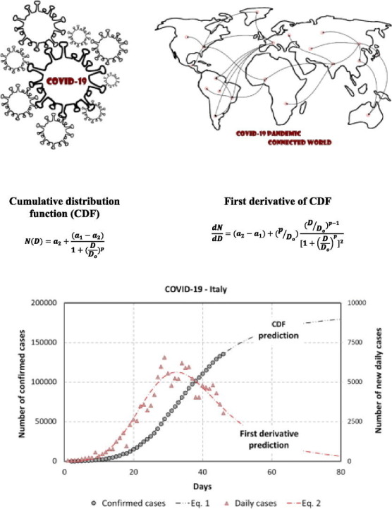
Graphical abstract

1. Introduction

Some European countries and more recently the United States of America has been making the headlines around the world as important epicenters of the widespread COVID-19 (CV-19) (severe acute respiratory syndrome - coronavirus 2) pandemic. Unfortunately, it is happening mainly by the high number of daily cases and deaths these countries have been facing and reporting (Saglietto et al., 2020).

A question that could be raised is: Could one, based on initial observations of the increasing rates of COVID-19 growth, estimate how the cases would evolve? It is a challenging and complex question, as many aspects should be considered for its answer, especially those associated with social mobility restrictions and community transmission characteristics. Even though, based on a reasonable mathematical model some scenarios can be drawn and serve as a warning on how the severity of one specific situation can evolve (Biswas and Sen, 2020).

It is well known and observed that as time passes, the number of CV-19 cases experiences a rapid rising followed by stabilization after some time. It presents what is called a step-like function behavior. Frequently, the exponential model of growth is chosen for fitting and forecasting future cases (Remuzzi and Remuzzi, 2020). Nevertheless, even a good prediction model will start to deviate from the actual data in just a few weeks and, therefore, without any adjustment become useless for this task. The idea of this study is to provide a more realistic growth model of confirmed CV-19 cases to give anyone conditions to promptly evaluate how restrictive mobility actions (as, for instance, social isolation) are changing the virus growing rates.

2. Theory

There is a very simple and concise mathematical function that behaves like a step-like function. It is known as the cumulative distribution function (CDF) whose expression is presented in Eq. (1) (Zandbergen and Chakraborty, 2006):

$$N\left(D\right)=a_2+\frac{\left(a_1-a_2\right)}{1+{\left(\frac{D}{D_o}\right)}^p}$$ (1)

where a₁, a₂, D_o, and p are adjustment parameters, and D is any particular day after the first CV-19 cases were detected.

Its first derivative dN/dD, presented in Eq. (2), provides the number of new cases to be expected using the adjusted parameters found in Eq. (1):

$$\frac{\mathit{dN}}{\mathit{dD}}=\left(a_2-a_1\right)+\left(\frac{p}{D_o}\right)\frac{{\left(\frac{D}{D_o}\right)}^{p-1}}{{\left[1+{\left(\frac{D}{D_o}\right)}^p\right]}^2}$$ (2)

3. Results and discussion

As declared free from new cases, China could be used as an example of the proposed model prediction (Eq. 1) to describe the behavior of the confirmed cases and confirmed new cases (Fig. 1 ).

Fig. 1.

The number of confirmed (circles) and new daily cases (triangles) in China. The red square dot indicates an unusual occurrence when 14 thousand new daily cases were confirmed in China (21st day of the pandemic). (For interpretation of the references to colour in this figure legend, the reader is referred to the web version of this article.)

It can be noticed that the model is well adjusted to the number of confirmed cases as r ² = 0.9912. The region poorest evaluated is probably related to an unusual event that happened in the 21st day of the pandemic when, differently from the other days, 14 thousand daily cases were officially confirmed in China (red square dot in Fig. 1) (Worldometers.info, 2020).

Based on the model, the Italian cases are presented in Fig. 2 .

Fig. 2.

The number of confirmed (circles) and new daily cases (triangles) in Italy. The dashed lines exhibit the model predictions calculated using Eq. 1 (black dashed line) and 2 (red dashed line). (For interpretation of the references to colour in this figure legend, the reader is referred to the web version of this article.)

Italy, unfortunately, made the headlines around the world because it was one of the first countries to publicize enormous daily death numbers. Recently, an article was published presenting asymmetrical epidemic curves, related to CV-19 cases in some European countries (Saglietto et al., 2020; Remuzzi and Remuzzi, 2020). The authors emphasized that some projections, based on an exponential model of growth, predicted more than 30 thousand cases for Italy by March 15, around 5 weeks after the first confirmed cases (Armocida et al., 2020; Remuzzi and Remuzzi, 2020).

It is known that the exponential model, besides producing a good estimate, is adequate to describe the number of confirmed cases only for a short period, in general, one or two weeks from the initiation of the pandemic, as it quickly starts to deviate from the actual numbers as time passes.

In Fig. 3 , the exponential model (EM) is compared to the actual numbers. The EM was obtained using pandemic information from the first 14 days of the confirmed cases. It is seen that the EM (Fig. 3, red dashed line), deviates more than 100% of the data on the 21st day, i. e. around one week after the EM was conceived.

Fig. 3.

Exponential model (EM) used for fitting the actual data up to 14 days from the first case. On the 21st day, the deviations from the actual data and the EM are larger than 100%.

Eqs. (1), (2) were also employed to fit the data from some other European countries (Spain, Germany, and Austria) as presented in Fig. 4 . As in the case of Italy, the dashed lines are only predictions calculated using the CDF and its derivative (Eqs. (1), (2)).

Fig. 4.

Eq. 1 (black dashed line) and 2 (red dashed line) employed for fitting some other European countries, Spain, Germany, and Austria. D_o is provided by Eq. 1. (For interpretation of the references to colour in this figure legend, the reader is referred to the web version of this article.)

Differences in extreme weather conditions can explain the differences observed between the virus spread in different countries. Recently, Tosepu et al. (2020) reported the influence of climatic conditions in the spread of CV-19 in Indonesia. As an example, the correlation between the confirmed and new confirmed cases with the predicted ones, picking Austria as an example, are presented in Fig. 5 .

Fig. 5.

Confirmed and predicted cases using Eqs. 1 and 2 (inset scatterplot) for Austria. A 1:1 line is presented in both figures.

The r² values from the correlations indicate that the predicted cases correlate better with the confirmed cases as compared to the new confirmed ones. It happens as the number of new confirmed cases, besides the visible trend, is significantly variable than the confirmed cases, as can be seen in Fig. 4.

The parameters of the CDF adjustment for some European countries and China are presented in Table 1 .

Table 1.

The obtained parameters from Eq. 1 for China and some European countries. Countries were placed in decreasing order of p magnitude.

Parameters	Austria	Spain	Belgium	Italy	Germany	China	Norway
a1	113	717	293	818	508	0	0
a2	14,530	203,651	38,448	186,092	167,377	86,545	18,122
Do	25.8	32.8	31.8	36.4	32.0	17.6	49.8
p	5.24	4.91	4.41	4.18	4.16	3.37	2.40

Parameters a₁ and a₂ are related to the extrapolation of the curves for small (pandemic emergence) and large (pandemic stabilization) values of D, respectively. D_o is near to the inflection of the pandemic curve (quite close to the maximum of the curve of the new cases, Eq. 2) and p is related to its growth rate. Larger values of p are related to a more abrupt growth of the pandemic curve at its beginning and vice-versa.

It can be noticed that except for China and Norway, the values of D_o and p are close to 30 and 4.5, respectively. The average of these parameters followed by their standard deviations are D _o = (32 ± 4) days and p = (4.6 ± 0.5). It means that the inflection of the curve of growth (Eq. 1) starts around 32 days after the first CV-19 cases are detected and the curve of new daily cases has its maximum around this day. The parameter p of this magnitude indicates that the CV-19 cases have a huge rate of growth at 2 or 3 weeks after the first detected ones.

As a final example, in Fig. 6 are presented examples of the curves generated by Eqs. (1), (2), for distinct combinations of values of p and D_o. For comparison reasons, a₁ and a₂ were chosen as 0 and 1, respectively. It means that the curve minimum and maximum were chosen as 0 and 1, respectively.

Fig. 6.

The effect of varying p (top) and D_o (bottom) values in Eq. 1 (solid line) and 2 (dashed line). D_o = 32 and p = 4.6 are the average values of these parameters for the European modeled cases.

From Fig. 6 it is seen that an increase in p (p from 3 to 6) makes the curve more inclined at the beginning of the process. Also, higher values of p made the peak of Eq. 2 more pronounced and less spread out (p = 6 as compared to the others). The effect of changing D_o delayed the inflection point and made the peak more diffuse (the curve was flattened). The consequence of diminishing D_o in Eq. 1 was to accelerate the process of reaching its ending (a ₁ = 1) too.

4. Concluding remarks

As a final consideration, the answer to the first question is that it is almost impossible to predict, based on the first cases of CV-19 (first 2 or 3 weeks), how the pandemic will evolve. It is related to many considerations that have to be taking into account as, for instance: the dynamic of the spread, demographic population, restrictions of social mobility, individual protection measures (use of protective masks and hygiene procedures), virus incubation time, transmission rates, meteorological factors, etc. Nevertheless, more realistic models can reveal reliable aspects related to pandemic evolution. Also, it can serve as a valuable tool, for decision-makers of any country, to investigate how protective measures are changing the evolution of the CV-19 cases.

CRediT authorship contribution statement

Fábio A.M. Cássaro:Conceptualization, Methodology, Writing - original draft.Luiz F. Pires:Investigation, Writing - original draft.

Declaration of competing interest

The authors declare that they have no known competing financial interests or personal relationships that could have appeared to influence the work reported in this paper.

References

- Armocida B., Formenti B., Ussai S., Palestra F., Missoni E. The Italian health system and the COVID-19 challenge. Lancet. 2020;S2468-2667(20):30074–30078. doi: 10.1016/S2468-2667(20)30074-8. [DOI] [PMC free article] [PubMed] [Google Scholar]
- Biswas K., Sen P. Space-time dependence of coronavirus (COVID-19) outbreak. arXiv. 2020;2003:03149. (v1) [Google Scholar]
- Remuzzi A., Remuzzi G. COVID-19 and Italy: what next? Lancet. 2020;395:1225–1228. doi: 10.1016/S0140-6736(20)30627-9. [DOI] [PMC free article] [PubMed] [Google Scholar]
- Saglietto A., D'Ascenzo F., Zoccai G.B., De Ferrari G.M. COVID-19 in Europe: the Italian lesson. Lancet. 2020;395:1110–1111. doi: 10.1016/S0140-6736(20)30690-5. (S0140-6736(20)30673-5) [DOI] [PMC free article] [PubMed] [Google Scholar]
- Tosepu R., Gunawan J., Effendy D.S., Ahmad L.O.A.I., Lestari H., Bahar H., Asfian P. Correlation between weather and COVID-19 pandemic in Jakarta, Indonesia. Sci. Total Environ. 2020;725 doi: 10.1016/j.scitotenv.2020.138436. [DOI] [PMC free article] [PubMed] [Google Scholar]
- Worldometers.info, 2020, (Delaware, U.S.A).
- Zandbergen P.A., Chakraborty J. Improving environmental exposure analysis using cumulative distribution functions and individual geocoding. Int. J. Health Geogr. 2006;5:23. doi: 10.1186/1476-072X-5-23. [DOI] [PMC free article] [PubMed] [Google Scholar]