Mathematical properties of linkage disequilibrium statistics defined by normalization of the coefficient $D=p_{AB}-p_A{p}_B$

Abstract

Background:

Many statistics for measuring linkage disequilibrium (LD) take the form of a normalization of the linkage disequilibrium coefficient D. Different normalizations produce statistics with different ranges, interpretations, and arguments favoring their use.

Methods:

Here, to compare the mathematical properties of these normalizations, we consider five of these normalized statistics, describing their upper bounds, the mean values of their maxima over the set of possible allele frequency pairs, and the size of the allele frequency regions accessible given specified values of the statistics.

Results:

We produce detailed characterizations of these properties for the statistics d and ρ, analogous to computations previously performed for r². We examine the relationships among the statistics, uncovering conditions under which some of them have close connections.

Conclusion:

The results contribute insight into LD measurement, particularly the understanding of differences in the features of different LD measures when computed on the same data.

1. Introduction

Linkage disequilibrium (LD) refers to the non-random association of the alleles at a pair of genetic loci. It manifests as a deviation of observed haplotype frequencies from the frequencies expected under the assumption that alleles at the two loci associate independently. As a fundamental concept in population genetics, LD appears in a wide variety of contexts, such as association mapping and detection of natural selection [1–5].

The original measure of LD for a pair of biallelic loci, one with alleles A and a and the other with alleles B and b, was $D=p_{AB}-p_A{p}_B,$ where p_A and p_B represent the frequencies of alleles A and B, respectively, and p_AB is the frequency of the two-locus haplotype containing alleles A and B [6]. The frequencies p_A and p_B can be measured for the two loci separately, each in the absence of information on the other locus, whereas evaluation of the frequency p_AB uses information on co-occurrence within individuals of alleles at the two loci.

Because LD is a property of a relationship between a pair of loci, values of the allele frequencies at the two loci under consideration can affect the potential strength of that relationship. This dependence is a recognized feature of LD measurement: soon after the initial development of the measure D, the quantity |D′| was introduced as a normalization of D that has the same maximal value irrespective of the allele frequencies at the constituent loci [7].

Many measures of LD have been proposed, each with different arguments favoring its use [1, 3, 8–12]. For example, the popular measure r² [13] has the property that it can be interpreted as a squared correlation coefficient between indicator variables for the presence of allele A at the first locus and allele B at the second locus. Each allelic indicator variable is a Bernoulli trial, so that the squared covariance in the numerator of r², D², is obtained by examining the probability that both indicator variables simultaneously equal 1. Features of r² in a population evolving according to a standard neutral model are closely related to the population recombination rate 4N_ec, where N_e is the effective population size and c is the recombination rate between two loci [14–15]. In addition, a calculation of the sample size necessary to detect disease association at a marker locus in linkage disequilibrium with a disease locus relies specifically on a measurement of r² between the marker and disease loci [3, 16].

The measure d [17] contains an asymmetry between the pair of loci that can be useful if ascertainment of haplotypes forces specific frequencies for one of the loci. This asymmetry is potentially of use in association mapping in the context of a case-control study, where the B/b locus is taken to contain the disease allele, with A/a being a marker locus [9, 18]. In this context, d can also be interpreted as the difference in the proportions of disease and normal alleles found on the same haplotype with a particular marker allele [9].

The measure ρ has been argued to be informative in a model-based perspective on LD, in which it is treated as the probability that a haplotype chosen at random descends without recombination from a population of haplotypes that excludes the aB haplotype [19]. Specifically, given a set of allele and haplotype frequencies, ρ satisfies

$$\rho \left[\begin{array}{cc}{p}_B& p_A-p_B\\ 0& 1-p_A\end{array}\right]+(1-\rho )\left[\begin{array}{cc}{p}_A{p}_B& p_A(1-p_B)\\ (1-p_A)p_B& (1-p_A)(1-p_B)\end{array}\right]=\left[\begin{array}{cc}{p}_{AB}& p_{Ab}\\ p_{aB}& p_{ab}\end{array}\right].$$ (1)

A fifth measure, a normalization of r² termed $r^2/r_{\max }^2$ [20], has the same property as |D′| that its maximum is invariant with respect to the values of p_A and p_B.

All of these normalized measures — $|D^{\prime }|,r^2,d,\rho ,\text{and}{r}^2/r_{\text{max}}^2$ — have numerators that are functions of D and denominators that are functions of the single-locus quantities p_A and p_B. The normalizations introduce different consequences for the maximal values of the statistics as functions of p_A and p_B [8, 20–21]. They also affect the symmetries of the statistics both with respect to exchanges of the two loci and with respect to exchanges of the alleles at one or both loci.

In applying LD statistics, many uses implement numerical cutoffs to assess if a desired degree of association has been met by a pair of loci, with only those locus pairs whose LD value exceeds the threshold regarded as having done so. For example, pairwise LD thresholds have been used in defining the boundaries of haplotype blocks [22–23]. They have also been applied to select tag SNP sets to assay in association studies, choosing tags by the number of non-tags with which they achieve a minimum LD cutoff and evaluating the fraction of non-tags that achieve an LD cutoff with at least one tag [24–25]. LD thresholds have also been employed for such purposes as visualizing tiered LD levels [26], pruning correlated markers in polygenic risk score calculations [27], and generating networks whose vertices represent loci and whose edges connect locus pairs with LD values exceeding a cutoff [28].

The frequent use of pairwise LD thresholds motivates studies of the implicit properties of allele frequencies forced by the thresholds, and more generally, of the way in which numerical values and interpretations of the various statistics depend on allele frequencies. This paper examines such properties and other mathematical features of the various D-based statistics. Although the statistics all range from 0 to 1, owing to their different normalizations and constraints, the meaning of a numerical value of one statistic can differ from the meaning of the same value of another statistic. Our goal is to characterize properties of the range, dependencies, and typical magnitudes of the measures, in order to assist in giving insight about values observed in empirical and theoretical studies of LD.

VanLiere and Rosenberg [20] studied the maximal value of r² as a function of p_A and p_B (see also [29]), in addition to considering such quantities as the mean maximal value of r² over the unit square for the pair of allele frequencies, the mean maximal value for r² over values of p_B for fixed values of p_A, and the set of permissible values of p_B given r² and p_A (see also [30]). With the current emphasis on rare variants in human genetics [31–32], a salient observation concerning r² is that if rare mutations occur at two loci on the same common haplotype in different individuals, then r² for the pair of loci is likely to have an extremely low value [33–34], complicating the use of r² in comparing LD across locus pairs. Here, we examine aspects of the mathematical properties of LD measures for each of the five normalized measures. We also consider the relationships between pairs of measures, finding that some pairs of measures are equal in particular scenarios.

2. Theory

2.1. Setting

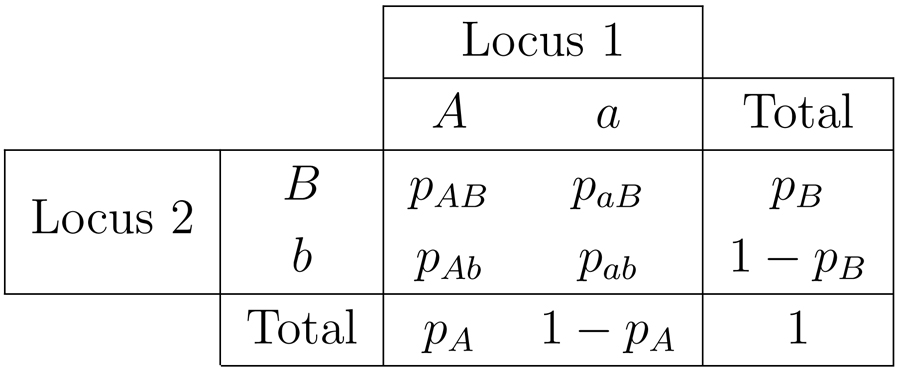
We consider two biallelic loci, locus 1 with alleles A and a, and locus 2 with alleles B and b. The population frequencies of these alleles are then given by $p_A,p_a=1-p_A,p_B,\text{and}{p}_b=1-p_B,$ respectively. Because both p_A and p_B lie in [0, 1], a set of frequencies can be characterized as a point in the unit square with axes p_A and p_B. For ease of notation, following VanLiere and Rosenberg [20], we split this square into octants S₁, S₂,...,S₈, as illustrated in Figure 1. The conditions on p_A and p_B that characterize these octants appear in Table 1. We henceforth assume that the loci are both polymorphic, so that p_A, p_a, p_B, and p_b all lie in (0, 1). The two pairs of alleles associate into four distinct haplotypes: AB, Ab, aB, and ab, with frequencies p_AB, p_Ab, p_aB, and p_ab, respectively (Table 2).

Figure 1:

A unit square showing all possible combinations of the frequencies p_A and p_B. The region is subdivided into eight octants S₁,...,S₈.

Table 1:

The eight octants in the space of possible allele frequencies, along with their associated $r_{\max }^2,|d{|}_{\max },\text{and}{\rho }_{\max }$ values.

Octant	Condition				pAB achieving maximal |D|	$r_{\max }^2$	|d|max	ρmax
	pA < $\frac{1}{2}$	pB < $\frac{1}{2}$	pA < pB	pA + pB < 1
S1	Yes	No	Yes	No	pA + pB − 1	$\frac{(1-p_A)(1-p_B)}{p_A{p}_B}$	$\frac{1-p_A}{p_B}$	-
S2	No	No	Yes	No	pA	$\frac{p_A(1-p_B)}{(1-p_A)p_B}$	$\frac{p_A}{p_B}$	-
S3	No	No	No	No	pB	$\frac{(1-p_A)p_B}{p_A(1-p_B)}$	-	-
S4	No	Yes	No	No	pA + pB − 1	$\frac{(1-p_A)(1-p_B)}{p_A{p}_B}$	-	1
S5	No	Yes	No	Yes	0	$\frac{p_A{p}_B}{(1-p_A)(1-p_B)}$	$\frac{p_A}{1-p_B}$	1
S6	Yes	Yes	No	Yes	pB	$\frac{(1-p_A)p_B}{p_A(1-p_B)}$	$\frac{1-p_A}{1-p_B}$	1
S7	Yes	Yes	Yes	Yes	pA	$\frac{p_A(1-p_B)}{(1-p_A)p_B}$	-	-
S8	Yes	Yes	Yes	Yes	0	$\frac{p_A{p}_B}{(1-p_A)(1-p_B)}$	-	-

Table 2:

Notation for the allele and haplotype frequencies for a pair of biallelic loci.

We consider parametric values for the allele frequencies, so that our interest is in LD statistics computed as functions of quantities $p_A,p_a,p_B,p_b,p_{AB},p_{Ab},p_{aB},\text{and}{p}_{ab}.$ This setting amounts to considering the statistics in an idealized setting of an infinite population.

2.2. The five normalized LD measures

As mentioned earlier, the most basic measure of LD is $D=p_{AB}-p_A{p}_B,$ the difference between the observed frequency of the AB haplotype and its expected frequency under independence of loci 1 and 2. Expressions for D can also be formulated using each of the three other possible combinations of alleles at the two loci (Ab, aB, and ab). The four formulations all give an identical value, up to a change in sign.

If no association exists between the two loci, then we expect $p_{AB}=p_A{p}_B,$ and hence D = 0. We consider several LD measures, each of which is a normalization of D. For instance, D′ is obtained by normalizing D by its maximal magnitude, given the sign of D:

$$D^{\prime }=\frac{D}{D_{\max }},\text{where}{D}_{\max }=\{\begin{array}{ll}\min [p_A(1-p_B),(1-p_A)p_B]\hfill & \text{if}D>0\hfill \\ \min [p_A{p}_B,(1-p_A)(1-p_B)]\hfill & \text{if}D<0\hfill \end{array}.$$ (2)

The r² measure is defined as D² normalized by the product of all four allele frequencies:

$$r^2=\frac{D^2}{p_A(1-p_A)p_B(1-p_B)}.$$ (3)

The next two LD measures represent the two ways in which D can be normalized by the product of two of the four allele frequencies. If the two frequencies represent alleles from the same locus, then we have d, given by Nei and Li [17]:

$$d=\frac{D}{p_B(1-p_B)}.$$ (4)

By convention, in an association mapping setting, locus 2 is designated as a disease locus, and hence B or b is regarded as a potential disease-causing allele.

If the two frequencies instead represent alleles from different loci, then we have ρ, given by Collins and Morton [35]:

$$\rho =\frac{D}{(1-p_A)p_B}.$$ (5)

Unlike D′ and r², both d and ρ introduce an asymmetry in the pair of loci by virtue of the choice of alleles assigned to their denominators.

Lastly, as was noted by VanLiere and Rosenberg [20], the maximal value of r² is constrained by the values of the allele frequencies p_A and p_B. Let $r_{\max }^2$ be the maximal value of r² possible given p_A and p_B. The measure $r^2/r_{\max }^2,$ introduced by VanLiere and Rosenberg [20], is then simply equal to r² normalized by $r_{\max }^2$.

2.3. Prescribed domains

The measures D′ and r² can be applied for all values of p_A and p_B in (0,1), that is, in all octants in Figure 1. $r^2/r_{\max }^2,$ being derived from r², also has all octants available. However, d and ρ are defined only on part of the domain (0, 1) × (0, 1). For d, because locus 2 is usually taken to be a disease locus—with one relatively rare allele—and locus 1 is the marker locus, it is assumed that min(p_B, p_b) ⩽ min(p_A, p_a). This assumption restricts d to S₁, S₂, S₅, and S₆. For ρ, the allele frequencies are assigned labels such that $D⩾0,p_{aB}⩽p_{Ab},p_B⩽p_A,\text{and}{p}_B⩽1-p_B$ [19]. Note that p_aB ⩽ p_Ab is equivalent to $p_B⩽p_A,\text{as}{p}_{aB}=p_B-p_{AB}\text{and}{p}_{Ab}=p_A-p_{AB}.$ Together, these conditions restrict the available octants to S₄, S₅, and S₆. Domain restrictions are summarized in Table 3, and for d and ρ, we restrict our subsequent analysis to octants in which these measures apply.

Table 3:

Octants of the allele frequency space in which the different linkage disequilibrium measures can be applied.

Octant	D′	r2	d	ρ	$r^2/r_{\max }^2$
S1	Yes	Yes	Yes	No	Yes
S2	Yes	Yes	Yes	No	Yes
S3	Yes	Yes	No	No	Yes
S4	Yes	Yes	No	Yes	Yes
S5	Yes	Yes	Yes	Yes	Yes
S6	Yes	Yes	Yes	Yes	Yes
S7	Yes	Yes	No	No	Yes
S8	Yes	Yes	No	No	Yes

2.4. Upper bounds, mean maximum values, and accessible regions

We are interested in analyzing mathematical properties of the five LD measures. Because the magnitude of these measures is the quantity of interest, we work with the absolute values $|D^{\prime }|\text{and}|d|.r^2\text{and}{r}^2/r_{\max }^2$ are always non-negative owing to the fact that D² is used in their expressions, and ρ is always non-negative because its definition requires $D⩾0.$

We seek to determine the upper bound, mean maximal value, and accessible region for each of the five measures, given the values of p_A and p_B. The mean maximum $\mathbb{E}[m_{\max }]$ of a measure m is defined as its average maximum value, assuming $(p_A,p_B)$ follows a bivariate uniform distribution on the permissible domain over which m applies. Its accessible region for a constant $c\in [0,1],p_m(c),$ is defined as the proportion of the domain in which the upper bound for the measure is greater than or equal to c.

To determine these mathematical properties, we first must choose a value of p_AB that maximizes |D|, because all other variables in the expressions for the five statistics are fixed given p_A and p_B. The values of p_AB that achieve this maximum are the same as those given by VanLiere and Rosenberg [20] for finding the upper bound on r² (Figure 2A), because |D| is maximized if and only if D² is maximized. Hence, on S₁ and S₄, the maximum |D| occurs if $p_{AB}=p_A+p_B-1;$ on S₂ and S₇, if p_AB = p_A; on S₃ and S₆, if p_AB = p_B; and on S₅ and S₈, if p_AB = 0. These values appear in Table 1. For all five measures, the values of $\mathbb{E}[m_{\max }]\text{and}{p}_m(c)$ appear in Table 4.

Figure 2:

$r_{\max }^2$ and |d|_max as functions of p_A and p_B. (A) Contour plot of $r_{\max }^2$. (B) Contour plot of |d|_max. The plots consider the maximum over all possible values of p_AB. The functions plotted appear in Table 1. |d| is defined only in octants S₁, S₂, S₅, and S₆.

Table 4:

Mean maximum values and accessible regions for the five measures. The mean maximum value of a measure is its average maximum value over its prescribed domain, assuming p_A and p_B are independent and uniformly distributed over the domain. The accessible region of a measure for a constant c ∈ [0, 1] is defined as the proportion of the applicable domain in which the upper bound for the measure is greater than or equal to c.

	Mean maximum value	Accessible region
|D′|	1	1
r2	2π2/3 − 4(ln 2)2 + 4 ln 2 − 7 ≈ 0.43051	1 + $\frac{4c}{1-c}$ + $\frac{8c\text{ln}(\frac{1}{2}+\frac{1}{2}c)}{{(1-c)}^2}$
|d|	$\frac{3}{2}$ − ln 2 ≈ 0.80685	1, if c ⩽ 0.5; $\frac{(4c-1)(1-c)}{c}$, if c > 0.5
ρ	1	1
$r^2/r_{\max }^2$	1	1

|D′|: Because |D′| is simply |D| normalized by its maximum value D_max, both its upper bound and the mean maximum $\mathbb{E}$[|D′|_max] are equal to 1. Furthermore, its accessible region p_|D′|(c) is also 1, irrespective of the value of c.

r²: The upper bound of r² as a function of p_A and p_B, for each octant S₁,...,S₈, was calculated in eqs. 2–5 of VanLiere and Rosenberg [20]. These results appear in Table 1, and a contour plot of $r_{\max }^2$ is reproduced in Figure 2A. In addition, VanLiere and Rosenberg [20] derived the mean maximum of r², obtaining $\mathbb{E}[r_{\max }^2]=2{\pi }^2/3-4{(\ln 2)}^2+4\ln 2-7\approx 0.43051,$ as well as its accessible region, which is

$$p_{r^2}(c)=1+\frac{4c}{1-c}+\frac{8c\ln \left(\frac{1}{2}+\frac{1}{2}c\right)}{{(1-c)}^2}.$$ (6)

A plot of p_r²(c) appears in Figure 3.

Figure 3:

The portion of the permissible allele frequency space where r² and |d| can exceed a specific value of c, as a function of c. p_r²(c) is taken from eq. 6, p_|d|(c) is taken from eq. 14, and both functions appear in Table 4.

|d|: By substituting the appropriate value of p_AB into the expression for |d|, we obtain |d|_max as a function of p_A and p_B in octants S₁, S₂, S₅, and S₆:

$$S_1:|d{|}_{\max }(p_A,p_B)=\frac{|p_A+p_B-1-p_A{p}_B|}{p_B(1-p_B)}=\frac{1-p_A}{p_B}$$ (7)

$$S_2:|d{|}_{\max }(p_A,p_B)=\frac{p_A-p_A{p}_B}{p_B(1-p_B)}=\frac{p_A}{p_B}$$ (8)

$$S_5:|d{|}_{\max }\left(p_A,p_B\right)=\frac{|0-p_A{p}_B|}{p_B\left(1-p_B\right)}=\frac{p_A}{1-p_B}$$ (9)

$$S_6:|d{|}_{\max }\left(p_A,p_B\right)=\frac{p_B-p_A{p}_B}{p_B\left(1-p_B\right)}=\frac{1-p_A}{1-p_B}.$$ (10)

These results are summarized in Table 1. Figure 2B shows a contour plot of ${|d|}_{\max }$ in S₁, S₂, S₅, and S₆, combining eqs. 7–10. We note some similarities, as well as some differences, with the plot of $r_{\max }^2$ in Figure 2A. Examining the characteristic X-shape of the figure, we see that ${|d|}_{\max }$ can equal 1 if and only if the allele frequencies are identical at the two loci, p_A = p_B or p_A = p_b, as is the case with $r_{\max }^2$. However, instead of having a symmetric shape over all octants, ${|d|}_{\max }$ is symmetric with respect to an exchange of p_A and p_a or p_B and p_b, but not with respect to an exchange of p_A and p_B (and thus also p_a and p_b) or p_A and p_b (and thus also p_a and p_B). Its shape is symmetric over S₁, S₂, S₅, and S₆, the four octants on which it can be calculated. Unlike $r_{\max }^2$, ${|d|}_{\max }$ does not approach 0 as p_B approaches either 0 or 1. This feature enables |d| to maintain a considerable range of allowable values, even if the minor allele frequency (MAF) at locus 2 is low, as is likely the case in a mapping study in which locus 2 is regarded as causal for a rare disease.

We can quantify the difference in range for |d| and r² by comparing the mean maximum value of |d| to that of r². First, we compute the volume V₂, which we define to be the volume of |d|_max over the octant S₂:

$$\begin{gathered} V_2={\int }_{\frac{1}{2}}^1{\int }_{p_A}^1\frac{p_A}{p_B}d{p}_{B}d{p}_A \\ =\frac{3}{16}-\frac{1}{8}\ln 2\approx \mathrm{0.10086.} \end{gathered}$$ (11)

Owing to symmetry, V₂ is equal to corresponding values V₁, V₅, and V₆. Assuming a uniform joint distribution of p_A and p_B over the octants S₁, S₂, S₅, and S₆, and noting that these octants have a total area $\frac{1}{2}$, the mean maximum value of $|d{|}_{\max }$ is

$$\begin{gathered} \mathbb{E}\left[|d{|}_{\max }\right]=4V_2/\frac{1}{2} \\ =\frac{3}{2}-\ln 2\approx \mathrm{0.80685.} \end{gathered}$$ (12)

This value exceeds $\mathbb{E}[r_{\max }^2]\approx 0.43051$ derived by VanLiere and Rosenberg [20] under the same assumption of a uniform distribution on the domain, suggesting that |d| can achieve a high magnitude over a considerably larger portion of the allele frequency space than is seen for r². To quantify this difference, we calculate the accessible region p_|d|(c). We first focus on S₆, and extend the result to the remaining octants using symmetry.

Let A₆ denote the area of the portion of S₆ in which |d|_max ⩾ c. Using eq. 10, the portion of S₆ in which |d|_max ⩾ c satisfies p_B ⩾ (p_A + c − 1)/c. We now set up an integral to calculate the complement of the desired area, the area of the portion of S₆ in which |d|_max ⩾ c. Observe from Figure 2B that in S₆, for $c⩾\frac{1}{2},$ the horizontal plane $|d{|}_{\max }=c$ intersects the upper bound at $p_A=1-c\text{if}{p}_B=0.$ Therefore, we have

$$\begin{gathered} \frac{1}{8}-A_6={\int }_{1-c}^{\frac{1}{2}}{\int }_0^{\frac{p_A+c-1}{c}}1d{p}_{B}d{p}_A=\frac{{(2c-1)}^2}{8c} \\ {A}_6=\frac{(4c-1)(1-c)}{8c}. \end{gathered}$$ (13)

For $c⩽\frac{1}{2},$ all points in octants S₁, S₂, S₅, and S₆ have ${|d|}_{\max }⩾c$ (Figure 2B). Hence, in this situation, $p_{|d|}(c)$ is simply 1. For $c⩾\frac{1}{2},$ applying eq. 13,

$$\begin{gathered} p_{|d|}(c)=4A_6/\frac{1}{2} \\ =\frac{(4c-1)(1-c)}{c}. \end{gathered}$$ (14)

The piecewise function p_|d|(c) appears in Figure 3, alongside a plot of p_r²(c) from eq. 6. The permissible fraction of the frequency space for |d| decreases more slowly as a function of c than does the corresponding function for r².

ρ: For the upper bound on ρ, the following conditions all must be satisfied when assigning labels to the alleles: $D⩾0,p_B⩽p_A,\text{and}{p}_B⩽1-p_B$ [19, 36]. The latter two conditions imply that ρ applies only in S₄, S₅, and S₆. The condition $p_B⩽p_A\text{implies}{p}_B-p_A{p}_B⩽p_A-p_A{p}_B,$ which in turn implies $(1-p_A)p_B⩽p_A(1-p_B).$ This result, in addition to the requirement that D ⩾ 0, indicates that ρ is exactly equal to |D′| under the conditions in which ρ applies. Consequently, the upper bound of ρ, its mean maximum $\mathbb{E}$[ρ_max], and its accessible region p_ρ(c) all equal 1.

${\mathit{r}}^{\mathbf{2}}/{\mathit{r}}_{\mathbf{max}}^{\mathbf{2}}\mathbf{:}$ The upper bound, the mean maximum $\mathbb{E}[{\{r^2/r_{\max }^2\}}_{\max }].$ and the accessible region $p_r^2/r_{\max }^2(c)$ all equal 1, by the definition of the statistic as r² normalized by $r_{\max }^2.$

2.5. Mean maximum of r² and |d| under a beta distribution

In Section 2.4, we examined the mean maximum of the five measures, assuming (p_A, p_B) follows a bivariate uniform distribution. For r² and |d|, the two measures that do not have a mean maximum of 1, we can also calculate their mean maximum value under less restrictive assumptions. We now assume p_A and p_B follow independent beta distributions. To preserve symmetry between loci and exchangeability of the alleles at a locus, we consider p_A, p_B ~ Beta-(α, α), and compute $\mathbb{E}$[|d|_max] and $\mathbb{E}[r_{\max }^2]$ as functions of α.

By analogy with eq. 12, again using octant S₂, we can set up an integral for $\mathbb{E}$[|d|_max]:

$$\begin{gathered} \mathbb{E}\left[|d{|}_{\max }\right]=8{\int }_{\frac{1}{2}}^1{\int }_{p_A}^1\frac{p_A}{p_B}\frac{p_A^{\alpha -1}{\left(1-p_A\right)}^{\alpha -1}}{\text{B}(\alpha ,\alpha )}\frac{p_B^{\alpha -1}{\left(1-p_B\right)}^{\alpha -1}}{\text{B}(\alpha ,\alpha )}d{p}_{B}d{p}_A \\ =\frac{8}{{[\text{B}(\alpha ,\alpha )]}^2}{\int }_{\frac{1}{2}}^1{\int }_{p_A}^1\frac{p_A}{p_B}{\left(p_A-p_A^2\right)}^{\alpha -1}{\left(p_B-p_B^2\right)}^{\alpha -1}d{p}_{B}d{p}_A. \end{gathered}$$ (15)

Here, B(α, α) = [Γ(α)]²/Γ(2α). To compute $\mathbb{E}\left[r_{\max }^2\right],\text{we use}{r}_{\max }^2\text{on}{S}_2$ (Table 1):

$$\begin{gathered} \mathbb{E}\left[r_{\max }^2\right]=8{\int }_{\frac{1}{2}}^1{\int }_{p_A}^1\frac{p_A\left(1-p_B\right)}{\left(1-p_A\right)p_B}\frac{p_A^{\alpha -1}{\left(1-p_A\right)}^{\alpha -1}}{\text{B}(\alpha ,\alpha )}\frac{p_B^{\alpha -1}{\left(1-p_B\right)}^{\alpha -1}}{\text{B}(\alpha ,\alpha )}d{p}_{B}d{p}_A \\ =\frac{8}{{[\text{B}(\alpha ,\alpha )]}^2}{\int }_{\frac{1}{2}}^1{\int }_{p_A}^1\frac{p_A\left(1-p_B\right)}{\left(1-p_A\right)p_B}{\left(p_A-p_A^2\right)}^{\alpha -1}{\left(p_B-p_B^2\right)}^{\alpha -1}d{p}_{B}d{p}_A. \end{gathered}$$ (16)

We evaluate eqs. 15 and 16 numerically, using values of α ranging from 0.2 to 5. The results appear in Figure 4. Low values of α imply that the distribution of allele frequencies is skewed toward loci with a low MAF, whereas high α values correspond to greater density in loci with a high MAF. Note that setting α = 1 gives a uniform distribution and recovers the values derived in Section 2.4 for the case of p_A, p_B ~ Uniform-(0,1).

Figure 4:

Mean maximum value of r² and |d|, if p_A and p_B are drawn from independent Beta-(α, α) distributions. The dotted line indicates α = 1, which gives values that are identical to the case in which p_A and p_B are drawn from independent Uniform-(0, 1) distributions.

From Figure 4, we observe that $\mathbb{E}[r_{\max }^2]$ varies considerably as a function of the allele frequency distribution, whereas $\mathbb{E}$[|d|_max] is more stable as α changes.

2.6. The five measures as functions of p_AB for fixed p_A, p_B

For most of our subsequent calculations, to facilitate comparison, we restrict our analysis to values of p_A and p_B in S₆, as all five measures have S₆ in their prescribed domains. Any point not in S₆ can be mapped to a point in S₆ by performing one or more of a set of transformations: (i) reflection over $p_B=\frac{1}{2}$ (corresponding to exchanging the p_A and p_a labels), (ii) reflection over $p_A=\frac{1}{2}$ (exchanging the p_B and p_b labels), and (iii) reflection over the p_A = p_B line (exchanging the p_A and p_B labels, and thus also the p_a and p_b labels).

We first compare how each measure varies with the haplotype frequency p_AB. Figure 5 illustrates $|D^{\prime }|,r^2,|d|,\text{and}{r}^2/r_{\max }^2$ as functions of the haplotype frequency p_AB, for fixed values of p_A and p_B. In this analysis, ρ is omitted because under the conditions in which it applies, it is exactly equal to |D′|. Each of the measures has a value of 0 in the case of linkage equilibrium, at which p_AB = p_Ap_B. Using p_AB = p_Ap_B as a reference point, we can split the plots for each of the measures into two portions: the right arm, where $p_{AB}⩾p_A{p}_B(\text{or}D⩾0,$ corresponding to the case with an excess of haplotypes containing both minor alleles), and the left arm, where p_AB ⩽ p_Ap_B (or D ⩽ 0, corresponding to the case with a deficit of haplotypes containing both minor alleles).

Figure 5:

Values of linkage disequilibrium statistics as functions of the haplotype frequency p_AB, for fixed values of p_A and p_B in S₆.

|D′|: |D′| varies linearly with p_AB. However, its left and right arms are in general not symmetric about the line p_AB = p_Ap_B; the absolute value of the derivative of |D′| as a function of p_AB differs in the two arms. This phenomenon results from the different normalizations applied in obtaining D′, depending on whether D is positive or negative. The left and right arms of |D′| are symmetric only if $p_A=\frac{1}{2},p_B=\frac{1}{2},$ or both. The value of |D′| can always reach 1 irrespective of whether the haplotype containing both minor alleles is in excess or in deficit; in general, no such result holds for the other three measures.

r²: r² varies quadratically as a function of p_AB, with the measure increasing at a faster rate the further p_AB is from p_Ap_B. As reported by VanLiere and Rosenberg [20], in S₆, r² can only reach 1 if p_A = p_B, and even then only if an excess of haplotypes containing both minor alleles occurs. Finally, ignoring the truncation imposed by the lower limit of p_AB = 0, the arms of r² are symmetric with respect to the line p_AB = p_Ap_B.

|d|: |d|, like |D′|, varies linearly as a function of p_AB. However, unlike for |D′|, the left and right arms of |d| are symmetric, and they have the same absolute value of the derivative as a function of p_AB. This pattern occurs because |d| does not necessarily have to reach 1 at the points where p_AB lies at its maximum or minimum values, given p_A and p_B. Like r², |d| can only reach 1 on its right arm if p_A = p_B. As a result, |D′| = |d| if p_A = p_B and D ⩾ 0, as can be observed from Figure 5.

${\mathit{r}}^{\mathbf{2}}/{\mathit{r}}_{\mathbf{max}}^{\mathbf{2}}:r^2/r_{\max }^2$ varies quadratically as a function of p_AB, but increases more quickly compared to r² as p_AB moves away from p_Ap_B. It can always reach 1 irrespective of the values of p_A and p_B but does so only if the haplotype containing both minor alleles is in excess. If p_A = p_B, then $r^2/r_{\max }^2=r^2,$ as the maximum of r² is 1 in this case.

Comparison:

In general, for all values of p_A, p_B, and p_AB, $|D^{\prime }|⩾|d|⩾r^2.$ To demonstrate this, we first show that |D′| ⩾ |d|. Consider D > 0, where D is normalized by min [p_A(1 − p_B), (1 − p_A)p_B] in the calculation of $|D^{\prime }|.\text{If}{p}_A⩾p_B,\text{then}{p}_A\left(1-p_B\right)⩾p_B\left(1-p_B\right)⩾\left(1-p_A\right)p_B,\text{but if}{p}_A⩽p_B,\text{then}{p}_A\left(1-p_B\right)⩽p_B\left(1-p_B\right)⩽\left(1-p_A\right)p_B.\text{In}\text{either case,}{p}_B\left(1-p_B\right)⩾\min \left[p_A\left(1-p_B\right),\left(1-p_A\right)p_B\right],\text{and therefore}|D^{\prime }|⩾|d|.$ A similar calculation shows also that $|D^{\prime }|⩾|d|\text{if}D<0.$

To see that $|d|⩾r^2$ where |d| applies (S₁, S₂, S₅, S₆), we show $r^2/|d|⩽1.$ We have

$$\frac{r^2}{|d|}=\frac{|D|}{p_A\left(1-p_A\right)}=\frac{|p_{AB}-p_A{p}_B|}{p_A\left(1-p_A\right)}.$$ (17)

Consider S₆, where p_A ⩾ p_B and p_AB = p_B maximizes |D| (Table 1):

$$\frac{|p_{AB}-p_A{p}_B|}{p_A(1-p_A)}⩽\frac{p_B-p_A{p}_B}{p_A(1-p_A)}=\frac{p_B}{p_A}.$$ (18)

Because $p_A⩾p_B,r^2/|d|⩽1.$ Eq. 18 and other similar calculations for S₁, S₂, and S₅ show that $|d|⩾r^2$ for all possible values of p_A and p_B.

2.7. Mean LD values given fixed p_A and p_B

In Section 2.4, we have described upper bounds of the five measures given values of p_A and p_B. We have also computed the mean of the maximum value. Next, we specify a distribution on p_AB and calculate the mean values of the measures over the possible domain.

For this section, we again use S₆; analogous results for other octants follow the same framework. Because p_B ⩽ p_A in S₆, p_AB lies in [0, p_B]. If we further assume p_AB ~ Uniform-(0, p_B), then we can compute the mean value of each LD measure as a function of p_A and p_B. For completeness, associated variances are derived in the Appendix.

$|{\mathit{D}}^{\prime }|\mathbf{:}D>0\text{if}{p}_{AB}>p_A{p}_B,\text{and}D<0\text{if}{p}_{AB}<p_A{p}_B.$ We split the integral for the mean to account for both cases. If p_AB is distributed uniformly on (0, p_B), then $\mathbb{E}\left[|D^{\prime }|\right]$ has a constant value of $\frac{1}{2}$, and does not depend on p_A or p_B.

$$\begin{gathered} \mathbb{E}\left[|D^{\prime }|\right]=\frac{1}{p_B}\left[{\int }_0^{p_A{p}_B}\frac{p_A{p}_B-p_{AB}}{p_A{p}_B}d{p}_{AB}+{\int }_{p_A{p}_B}^{p_B}\frac{p_{AB}-p_A{p}_B}{\left(1-p_A\right)p_B}d{p}_{AB}\right] \\ =\frac{1}{2}. \end{gathered}$$ (19)

r²: For r², it is not necessary to split the integral.

$$\begin{gathered} \mathbb{E}\left[r^2\right]=\frac{1}{p_B}{\int }_0^{p_B}\frac{{\left(p_{AB}-p_A{p}_B\right)}^2}{p_A\left(1-p_A\right)p_B\left(1-p_B\right)}d{p}_{AB} \\ =\frac{p_B\left(1-3p_A+3p_A^2\right)}{3p_A\left(1-p_A\right)\left(1-p_B\right)}. \end{gathered}$$ (20)

The result is plotted in Figure 6A.

Figure 6:

Mean value of three linkage disequilibrium statistics in S₆ as functions of p_A and p_B, assuming p_AB ~ Uniform-$\left(0,p_B\right).(\text{A})r^2.(\text{B})|d|.(\text{C})r^2/r_{\text{max}}^2$.

|d|: For d, we again split the integral as we did for |D′|.

$$\begin{gathered} \mathbb{E}[|d|]=\frac{1}{p_B}\left[{\int }_0^{p_A{p}_B}\frac{p_A{p}_B-p_{AB}}{p_B\left(1-p_B\right)}d{p}_{AB}+{\int }_{p_A{p}_B}^{p_B}\frac{p_{AB}-p_A{p}_B}{p_B\left(1-p_B\right)}d{p}_{AB}\right] \\ =\frac{1-2p_A+2p_A^2}{2\left(1-p_B\right)}. \end{gathered}$$ (21)

The result is plotted in Figure 6B.

${\mathit{r}}^{\mathbf{2}}/{\mathit{r}}_{\mathbf{max}}^{\mathbf{2}}\mathbf{:}$ The result appears in Figure 6C. Note that in octant $S_6,\mathbb{E}\left[r^2/r_{\max }^2\right]$ is a function of only p_A (or in general, allele frequencies at the locus with the higher MAF).

$$\begin{gathered} \mathbb{E}\left[r^2/r_{\max }^2\right]=\frac{1}{p_B}{\int }_0^{p_B}\frac{\frac{{\left(p_{AB}-p_A{p}_B\right)}^2}{p_A\left(1-p_A\right)p_B\left(1-p_B\right)}}{\frac{\left(1-p_A\right)p_B}{p_A\left(1-p_B\right)}}d{p}_{AB} \\ =\frac{1-3p_A+3p_A^2}{3{\left(1-p_A\right)}^2}. \end{gathered}$$ (22)

$\mathbb{E}\left[r^2/r_{\max }^2\right]$ varies less across the domain for p_A than do $\mathbb{E}$[r²] and $\mathbb{E}$[|d|].

2.8. Constraints on one allele frequency given an LD value and the allele frequency at the other locus

In this section, we examine for each of the five LD measures the allowable values of one allele frequency (either p_A or p_B) while fixing the allele frequency at the other locus and specifying the value of the LD measure. Owing to symmetry in the loci, for $|D^{\prime }|,r^2,\text{and}{r}^2/r_{\max }^2,$ fixing p_A is equivalent to fixing p_B, and we need only examine one case. For |d| and ρ, owing to asymmetries in the formulation of the measures, two cases must be considered. For the calculations in this section, we assume for convenience that p_A and p_B are the minor allele frequencies (octants S₆ and S₇), and that the constraints on the major allele frequencies will follow accordingly. The results of this section are summarized in Table 5.

Table 5:

Constraints on one allele frequency given an LD value and allele frequency at the other locus, for the five measures. Here, we assume $p_A,p_B⩽\frac{1}{2}$. Owing to symmetry in the loci, for $|D^{\prime }|,r^2,\text{and}{r}^2/r_{\max }^2,$ fixing p_A is equivalent to fixing p_B.

	Fixed allele frequency
	pA	pB
|D′|	0 ⩽ pB ⩽ 1	0 ⩽ pA ⩽ 1
r2	$\frac{r^2{p}_A}{1+r^2{p}_A-p_A}⩽p_B⩽\min \left(\frac{1}{2},\frac{p_A}{r^2-r^2{p}_A+p_A}\right)$	$\frac{r^2{p}_B}{1+r^2{p}_B-p_B}⩽p_A⩽\min \left(\frac{1}{2},\frac{p_B}{r^2-r^2{p}_B+p_B}\right)$
|d|	$\max \left(0,\frac{p_A+|d|-1}{|d|}\right)⩽p_B⩽p_A$	$p_B⩽p_A⩽\min \left(\frac{1}{2},1-|d|+|d|p_B\right)$
ρ	0 ⩽ pB ⩽ 1	0 ⩽ pA ⩽ 1
$r^2/r_{\max }^2$	0 ⩽ pB ⩽ 1	0 ⩽ pA ⩽ 1

Allowable values of p_B, given |D′| and p_A: Having a value of |D′| and a value of p_A does not constrain p_B, as all values of |D′| between 0 and 1 are accessible given a pair of allele frequencies p_A and p_B. This result can be shown from the fact that given p_A and p_B, |D′| is a continuous rational function of p_AB. Because 0 and 1 are the extreme values of |D′|, by the intermediate value theorem, |D′| can take on any value in [0, 1] (also see Figure 5).

Allowable values of p_B, given r² and p_A: Assuming that $p_A,p_B⩽\frac{1}{2},$ given p_A and r², the constraint on p_B is

$$\frac{r^2{p}_A}{1+r^2{p}_A-p_A}⩽p_B⩽\min \left(\frac{1}{2},\frac{p_A}{r^2-r^2{p}_A+p_A}\right).$$ (23)

This result has been previously reported in eqs. 10 and 11 of VanLiere and Rosenberg [20] and Table 2 of Wray [30].

Allowable values of p_B, given |d| and p_A: Because |d| is not symmetric in the two loci, we first assume |d| and p_A are specified, and solve for the range of p_B. Recalling that d applies only in S₁, S₂, S₅, and S₆, and assuming $p_A,p_B⩽\frac{1}{2},$ we consider S₆. From eq. 10,

$$\begin{gathered} |d|⩽\frac{1-p_A}{1-p_B} \\ {p}_B⩾\frac{p_A+|d|-1}{|d|}. \end{gathered}$$ (24)

Taking into account $0⩽p_B⩽p_A⩽\frac{1}{2},$ we have

$$\max \left(0,\frac{p_A+|d|-1}{|d|}\right)⩽p_B⩽p_A.$$ (25)

Allowable values of p_A, given |d| and p_B: Next, we assume |d| and p_B are specified, and solve for the range of p_A. In S₆, from eq. 10,

$$\begin{gathered} |d|⩽\frac{1-p_A}{1-p_B} \\ {p}_A⩽1-|d|+|d|p_B. \end{gathered}$$ (26)

Taking into account 0 $⩽p_B⩽p_A⩽\frac{1}{2},$ we have

$$p_B⩽p_A⩽\min \left(\frac{1}{2},1-|d|+|d|p_B\right).$$ (27)

The upper bound here corresponds to the upper bound for the “frequency difference” measure of LD reported in Table 2 of Wray [30], noting that labels p_A and p_B are reversed in that study. However, a difference exists between the reported lower bounds, which can be attributed to the fact that $p_A⩽\frac{1}{2}$ is not mandated by Wray [30].

Allowable values of p_B, given ρ and p_A: Because all values of ρ in [0, 1] can be reached with any given set of allele frequencies in the permissible domain, no additional constraint exists on p_B given ρ and p_A.

Allowable values of p_A, given ρ and p_B: For the same reason as in the case in which p_A is instead specified, no additional constraint exists on p_A given ρ and p_B.

Allowable values of p_B, given $r^2/r_{\max }^2$ and p_A: Being given a value of $r^2/r_{\max }^2$ and p_A does not constrain the values p_B can take, as all values of $r^2/r_{\max }^2$ in [0, 1] are accessible for a given set of allele frequencies p_A and p_B.

3. Data illustration

We now examine how LD distributions from data, as given by the various measures, relate to our bounds. We use the 1000 Genomes Project (data at http://csg.sph.umich.edu/abecasis/MACH/download/1000G-PhaseI-Interim.html), considering LD values on chromosome 22 of its pooled European population, consisting of 381 individuals: 87 Utah residents of Northern and Western European ancestry, 93 Finnish from Finland, 89 British from England and Scotland, 14 Iberians from Spain, and 98 Toscani from Italy. To ensure inclusion of locus pairs with substantial LD, calculations are restricted to pairs of loci that lie at most 1,000 base pairs apart. Once again, for ease of comparison, all pairs of allele frequency values outside S₆ are mapped to corresponding points within S₆.

3.1. Pairs of loci for which $|D^{\prime }|=1$

From 225,159 loci biallelic in the European data (of 494,975 loci in total), we obtain 1,742,020 pairs of loci separated by at most 1,000 base pairs. Of these, 1,465,140 pairs have $|D^{\prime }|=1$, indicating the presence of only two or three of the four possible haplotypes. Recalling that |D′| can reach 1 either if an excess or a deficit of haplotypes containing both minor alleles occurs, 349,837 locus pairs belong to the former case, and 1,115,303 to the latter.

r²: We now examine on S₆ how r² is distributed in relation to the upper bound. If |D′| = 1 for a pair of loci, then the r² value lies on one of two surfaces. If |D′| = 1 as the result of an excess of haplotypes containing both minor alleles, corresponding to p_AB = p_B, then r² lies on the surface that defines the upper bound on S₆, or

$$r^2=\frac{\left(1-p_A\right)p_B}{p_A\left(1-p_B\right)},$$ (28)

as given by eq. 4 in VanLiere and Rosenberg [20]. In S₆, with a deficit of haplotypes containing both minor alleles, |D′| = 1 is achieved if p_AB = 0, which results in the r² surface

$$r^2=\frac{{\left(0-p_A{p}_B\right)}^2}{p_A\left(1-p_A\right)p_B\left(1-p_B\right)}=\frac{p_A{p}_B}{\left(1-p_A\right)\left(1-p_B\right)}.$$ (29)

The surfaces and data points for these two cases appear in Figures 7A and 7B.

Figure 7:

The distributions of r², |d|, and $r^2/r_{\max }^2$ values calculated from data in S₆, when |D′| = 1. (A) r² values if p_AB = p_B, lying on the surface r² = (1 − p_A)p_B/[p_A(1 − p_B)]. (B) r² values if p_AB = 0, lying on the surface r² = p_Ap_B/[(1 − p_A)(1 − p_B)]. (C) |d| values if p_AB = p_B, lying on the surface |d| = (1 − p_A)/(1 − p_B). (D) |d| values if p_AB = 0, lying on the surface $|d|=\left(1-p_A\right)/\left(1-p_B\right).$ (E) $r^2/r_{\max }^2$ values if p_AB = p_B, lying on the surface $r^2/r_{\max }^2=1.(\text{F})r^2/r_{\max }^2$ values if p_AB = 0, lying on the surface $r^2/r_{\max }^2={\left[p_A/\left(1-p_A\right)\right]}^2.$

|d|: As was seen with r², |d| for a locus pair lies on one of two surfaces if |D′| = 1 (Figures 7C and 7D). Once again, if p_AB = p_B, then the associated surface is the upper bound of |d| on S₆, as in eq. 10. If p_AB = 0, then the points lie on

$$|d|=\frac{|0-p_A{p}_B|}{p_B\left(1-p_B\right)}=\frac{p_A}{1-p_B}.$$ (30)

${\mathit{r}}^{\mathbf{2}}/{\mathit{r}}_{\mathbf{max}}^{\mathbf{2}}\mathbf{:}$ Finally, we repeat the analysis for $r^2/r_{\max }^2$ values. If p_AB = p_B, then $r^2=r_{\max }^2$, and therefore $r^2/r_{\max }^2$ = 1. If instead p_AB = 0, then using eqs. 28 and 29, we obtain

$$\frac{r^2}{r_{\max }^2}=\frac{\frac{p_A{p}_B}{(1-p_A)(1-p_B)}}{\frac{(1-p_A)p_B}{p_A(1-p_B)}}={\left(\frac{p_A}{1-p_A}\right)}^2$$ (31)

The surfaces and points corresponding to these two cases appear in Figures 7E and 7F.

3.2. Pairs of loci for which |D′| < 1

In the special case in which |D′| = 1 for a pair of loci, we have seen that corresponding values for r², |d|, and $r^2/r_{\max }^2$ lie on well-defined surfaces. Although most locus pairs from our data fall within this category, for 276,880 of 1,742,020 pairs, |D′| < 1. For these pairs, we examine how the values of |D′|, r², |d|, and $r^2/r_{\max }^2$ are distributed within their ranges.

Recognizing that the four measures can exhibit different distribution patterns at different allele frequencies, we sample pairs of loci for which p_A and p_B have MAF values within four specified ranges, representing very low, low, intermediate, and high MAF: (0, 0.02], [0.04, 0.06], [0.24, 0.26], and [0.44, 0.46]. Distributions of values for the measures appear as a series of histograms in Figure 8, with each panel representing one pair of allele frequency ranges for p_A and p_B; because p_B ⩽ p_A in S₆, only 10 of the 16 possible combinations of joint allele frequency ranges are possible.

Figure 8:

The distributions of values of linkage disequilibrium statistics calculated from data in S₆, given specific ranges of values for p_A and p_B. For each of four windows for p_A and four windows for p_B, we divide points into bins based on their values of each of four statistics $(|D^{\prime }|,r^2,|d|,r^2/r_{\max }^2).$ The number of locus pairs falling into a pair of bins appears in the top right corner of the group of four histograms associated with the bin pair.

From Figure 8, we can observe a few properties of the distributions. First, in accordance with our theoretical results, the range of values for r² and |d| does not extend to 1 in the panels that are off the diagonal, where p_A = p_B is not possible. In particular, the limitation on the range of r² is more pronounced than that of |d|, when comparing within similar allele frequency ranges. This constraint also results in a large number of r² values being close to 0, especially if p_B is small (bottom row).

In addition, although we selected only locus pairs at most 1,000 bp apart, if p_B is small, then relatively few pairs have a high LD value. This result holds especially for r², but also for measures such as |D′| and $r^2/r_{\max }^2$ that always have upper bound 1. If one of the loci has a low MAF, then small changes in the haplotype frequency can have large effects on LD measures, especially those normalized to potentially reach 1 irrespective of the marginal allele frequencies (see also the p_B = 0.1 panels of Figure 5).

Comparing scenarios on the diagonal, where it is possible in principle for all four measures to achieve high LD values, we see that high LD values are more frequently observed for high and intermediate MAF than for low and very low MAF. For pairs of loci with low MAF, it is unusual for haplotypes to contain the rare allele at both loci, as the rare alleles likely result from relatively recent mutations that have taken place on the same common haplotype, but in different individuals. Thus, because the rare alleles are unlikely to co-occur, the nature of evolutionary descent makes it improbable that the LD-maximizing scenario that couples the rare variants will obtain. These considerations support a cautious perspective when interpreting LD measures in the case that one or both loci have a low MAF.

4. Discussion

In this paper, we have described the domains of five LD measures that are defined by normalizations of D or its square, with a function of p_A and p_B in the denominator. Based on these domains, we have calculated the upper bound, mean maximum, and accessible region for each of the five measures. Three of the measures (|D′|, ρ, and $r^2/r_{\max }^2$) can be considered “unrestricted,” in that their upper bound, mean maximum, and accessible region are all equal to 1. However, for the remaining two measures (r² and |d|), these values depend on the allele frequencies of the pair of loci under consideration.

For each of the five measures, its description, proposed usages, and mathematical properties are summarized in Table 6. The table provides examples illustrating how a measure’s mathematical properties can inform its use. For instance, |d| allows for a theoretically wider range of values compared to r², with a mean maximum of 0.80685 compared to 0.43051 for r². The increased range of |d| is evident in the analysis of genetic data, which suggests that empirical |d| values are more differentiated than corresponding r² values (Figure 8).

Table 6:

Description, usages, and mathematical properties of five LD measures for biallelic loci.

Statistic	Description	Noted usages in the literature	Mathematical properties
|D′|	Normalization of |D| by its theoretical maximum value for a given set of allele frequencies	Detecting “complete” LD (where one of the four haplotypes is absent), an indication of whether recombination has occurred between the two loci [11]	|D′| varies linearly as a function of pAB (Figure 5) Upper bound of 1 for all allele frequencies Assuming a uniform distribution of pAB over the range of values it can take, the mean and variance of |D′| are both constant values (eqs. 19 and 33)
r2	Squared correlation coefficient measure between allelic indicator variables	Testing for independence between a pair of loci by a χ2 test [16] Association studies, where a mathematical relationship exists between r2 and the sample size needed to detect association between a marker and disease phenotype [16]	r2 varies quadratically as a function of pAB (Figure 5) Low upper bound and small range of values if MAF is low (Figure 2A) Mean maximum value varies considerably as a function of the allele frequency distribution (Figure 4)
|d|	Difference in the proportions of disease and normal alleles found on the same haplotype with a particular marker allele	Association mapping for rare diseases in which case-control sampling is employed [9]	|d| varies linearly as a function of pAB (Figure 5) Upper bound has an intermediate value; measure still has a considerable range even at low MAF (Figure 2B) Mean maximum value relatively stable as a function of the allele frequency distribution (Figure 4)
ρ	Probability that a haplotype chosen at random descends without recombination from a population of haplotypes that excludes one of the four possible haplotypes	Mapping of marker association and localization of disease loci [19]	Identical to |D′| in the octants in which it can be applied
$r^2/r_{\max }^2$	Normalization of r2 by its theoretical maximum value for a given set of allele frequencies	If a range that is independent of allele frequency is desired, but the measure still maintains some connection to r2 [20]	$r^2/r_{\max }^2$ varies quadratically as a function of pAB (Figure 5) Upper bound of 1 for all allele frequencies Assuming a uniform distribution of pAB over the range of values it can take, the mean and variance of $r^2/r_{\max }^2$ both depend only on the locus with the larger MAF (eqs. 22 and 39)

In a sense, |d| can be considered a measure that is “intermediate” between |D′| and r². First, its value always lies between r² and |D′|. It also has properties in common each with r² and |D′|. Like |D′|, given p_A and p_B, |d| varies linearly as a function of p_AB, possessing a property that r² does not share. However, like r² but unlike |D′|, |d| is symmetric in p_AB around the linkage equilibrium value p_AB = p_Ap_B (Figure 5).

We have also identified situations in which some of these measures are equal to one another. Among the measures, ρ uniquely requires D ⩾ 0. This requirement, along with the conditions p_B ⩽ p_A and p_B ⩽ 1 − p_B, can be satisfied by (i) reflection over $p_A=\frac{1}{2}$ (exchanging the p_A and p_a labels), (ii) reflection over $p_B=\frac{1}{2}$ (exchanging p_B and p_b), or both. Under these prescribed conditions for the use of ρ, it exactly equals |D′|, a fact that had also been noted by Shete [36] and Mangin et al. [37]. Furthermore, |d| = |D′| if p_A = p_B and the haplotype containing both minor alleles is in excess. This result can be seen by observing the right arms of |D′| and |d| in plots along the diagonal of Figure 5, and also from noting that in the right arm, where D ⩾ 0, the normalizations $\min \left[p_A\left(1-p_B\right),\left(1-p_A\right)p_B\right]\text{and}{p}_B\left(1-p_B\right)\text{for}|D^{\prime }|$ and |d|, respectively, agree if p_A = p_B.

By quantifying the degree to which values for the different LD statistics change in response to shifts in allele and haplotype frequencies, the results provide context to the use of LD thresholds in various statistical genetics applications. Some uses impose thresholds in LD measures alongside minimal-MAF cutoffs [24–25, 27], and our results can be used to understand the behavior of the statistics in permissible ranges specified by simultaneous LD and MAF thresholds. Additionally, the results are useful for low-MAF loci, for which the rare alleles are unlikely to occur on the same haplotype. In particular, they illustrate that r² is the most tightly constrained measure (Figure 5, eq. 18), so that other measures might provide a broader range of values when computing LD statistics for loci with rare variants.

We note that we have focused on parametric aspects of LD measures rather than LD estimated from samples. Sampling properties can be examined, both in models that view alleles as draws from a parametric allele frequency distribution and in coalescent perspectives whose allele frequencies represent outcomes of a generative model (e.g. [38–40]). The functional forms of estimators can then potentially be combined with bounds on parametric LD measures to produce corresponding bounds on the estimators (e.g. [41, p. 1590]).

Many other measures of LD exist that are not included in our analysis [1, 3, 8–11]. Other measures are sometimes normalized by a quantity that includes a haplotype frequency, rather than a function of allele frequencies only, and thus do not lend themselves well to the framework in this paper. Similarly, LD measures used specifically in cases pertaining to multiallelic loci, such as the multiallelic |D′| [8, 42–43], require additional parameters. Of the LD measures that are described by a ratio of a function of D to a product of allele frequencies for biallelic loci, we have taken a comprehensive look at the most natural statistics with that form.

We initially assumed Uniform-(0,1) distributions on the allele frequencies to perform computations for the mean maximum of the various measures. This choice, as in VanLiere and Rosenberg [20], permits us to obtain mathematical insight into those measures across their prescribed ranges. In some applications, weighted distributions, such as the Beta-(α, α) distribution we subsequently used, can be applied in place of the uniform distribution.

Appendix

In this appendix, we provide the variances of $|D^{\prime }|,r^2,|d|,\text{and}{r}^2/r_{\max }^2,$ under the assumptions in Section 2.7. For computing the variances, we use eqs. 19, 20, 21, and 22 to supply the means $\mathbb{E}$[|D′|], $\mathbb{E}$[r²], $\mathbb{E}$[|d|], and $\mathbb{E}[r^2/r_{\max }^2]$, respectively.

$$\begin{gathered} \mathbb{E}\left[{|D^{\prime }|}^2\right]=\frac{1}{p_B}\left[{\int }_0^{p_A{p}_B}\frac{{\left(p_A{p}_B-p_{AB}\right)}^2}{p_A^2{p}_B^2}d{p}_{AB}+{\int }_{p_A{p}_B}^{p_B}\frac{{\left(p_{AB}-p_A{p}_B\right)}^2}{{\left(1-p_A\right)}^2{p}_B^2}d{p}_{AB}\right] \\ =\frac{1}{3}. \end{gathered}$$ (32)

$$\mathrm{Var}\left[|D^{\prime }|\right]=\frac{1}{3}-{\left(\frac{1}{2}\right)}^2=\frac{1}{12}.$$ (33)

$$\begin{gathered} \mathbb{E}\left[r^4\right]=\frac{1}{p_B}{\int }_0^{p_B}\frac{{\left(p_{AB}-p_A{p}_B\right)}^4}{p_A^2{\left(1-p_A\right)}^2{p}_B^2{\left(1-p_B\right)}^2}d{p}_{AB} \\ =\frac{\left[p_A^5+{\left(1-p_A\right)}^5\right]p_B^2}{5p_A^2{\left(1-p_A\right)}^2{\left(1-p_B\right)}^2}. \end{gathered}$$ (34)

$$\begin{gathered} \mathrm{Var}\left[r^2\right]=\frac{\left[p_A^5+{\left(1-p_A\right)}^5\right]p_B^2}{5p_A^2{\left(1-p_A\right)}^2{\left(1-p_B\right)}^2}-{\left[\frac{\left(1-3p_A+3p_A^2\right)p_B}{3p_A\left(1-p_A\right)\left(1-p_B\right)}\right]}^2 \\ =\frac{\left(4-15p_A+15p_A^2\right)p_B^2}{45p_A^2{\left(1-p_A\right)}^2{\left(1-p_B\right)}^2}. \end{gathered}$$ (35)

$$\begin{gathered} \mathbb{E}\left[|d{|}^2\right]=\frac{1}{p_B}{\int }_0^{p_B}\frac{{\left(p_{AB}-p_A{p}_B\right)}^2}{p_B^2{\left(1-p_B\right)}^2}d{p}_{AB} \\ =\frac{1-3p_A+3p_A^2}{3{\left(1-p_B\right)}^2}. \end{gathered}$$ (36)

$$\begin{gathered} \mathrm{Var}[|d|]=\frac{1-3p_A+3p_A^2}{3{\left(1-p_B\right)}^2}-{\left[\frac{1-2p_A+2p_A^2}{2\left(1-p_B\right)}\right]}^2 \\ =\frac{1-12p_A^2+24p_A^3-12p_A^4}{12{\left(1-p_B\right)}^2}. \end{gathered}$$ (37)

$$\begin{gathered} \mathbb{E}\left[{\left(r^2/r_{\max }^2\right)}^2\right]=\frac{1}{p_B}{\int }_0^{p_B}{\left[\frac{\frac{{\left(p_{AB}-p_A{p}_B\right)}^2}{p_A\left(1-p_A\right)p_B\left(1-p_B\right)}}{\frac{\left(1-p_A\right)p_B}{p_A\left(1-p_B\right)}}\right]}^{2}d{p}_{AB} \\ =\frac{p_A^5+{\left(1-p_A\right)}^5}{5{\left(1-p_A\right)}^4}. \end{gathered}$$ (38)

$$\begin{gathered} \mathrm{Var}\left[r^2/r_{\max }^2\right]=\frac{p_A^5+{\left(1-p_A\right)}^5}{5{\left(1-p_A\right)}^4}-{\left[\frac{1-3p_A+3p_A^2}{3{\left(1-p_A\right)}^2}\right]}^2 \\ =\frac{4-15p_A+15p_A^2}{45{\left(1-p_A\right)}^4}. \end{gathered}$$ (39)

References

- [1].Hudson RR: Linkage disequilibrium and recombination; in Balding DJ, Bishop M, Cannings C (eds): Handbook of Statistical Genetics. Chichester, Wiley, 2001, pp 309–324. [Google Scholar]
- [2].Nordborg M, Tavaré S: Linkage disequilibrium: what history has to tell us. Trends Genet 2002; 18: 83–90. [DOI] [PubMed] [Google Scholar]
- [3].McVean G: Linkage disequilibrium, recombination and selection; in Balding DJ, Bishop M, Cannings C (eds): Handbook of Statistical Genetics, ed 3 Chichester, Wiley, 2007, pp 909–944. [Google Scholar]
- [4].Slatkin M: Linkage disequilibrium — understanding the evolutionary past and mapping the medical future. Nat Rev Genet 2008; 9: 477–485. [DOI] [PMC free article] [PubMed] [Google Scholar]
- [5].Weir BS: Linkage disequilibrium and association mapping. Annu Rev Genomics Hum Genet 2008; 9: 129–142. [DOI] [PubMed] [Google Scholar]
- [6].Lewontin RC, Kojima K: The evolutionary dynamics of complex polymorphisms. Evolution 1960; 14: 458–472. [Google Scholar]
- [7].Lewontin RC: The interaction of selection and linkage.I. General considerations; heterotic models. Genetics 1964; 49: 49–67. [DOI] [PMC free article] [PubMed] [Google Scholar]
- [8].Hedrick PW: Genetic disequilibrium measures: proceed with caution. Genetics 1987; 117: 331–341. [DOI] [PMC free article] [PubMed] [Google Scholar]
- [9].Devlin B, Risch N: A comparison of linkage disequilibrium measures for fine-scale mapping. Genomics 1995; 29: 311–322. [DOI] [PubMed] [Google Scholar]
- [10].Sabatti C, Risch N: Homozygosity and linkage disequilibrium. Genetics 2002; 160: 1707–1719. [DOI] [PMC free article] [PubMed] [Google Scholar]
- [11].Mueller JC: Linkage disequilibrium for different scales and applications. Brief Bioinform 2004; 5: 355–364. [DOI] [PubMed] [Google Scholar]
- [12].Zapata C: On the uses and applications of the most commonly used measures of linkage disequilibrium from the comparative analysis of their statistical properties. Hum Hered 2011; 71: 186–195. [DOI] [PubMed] [Google Scholar]
- [13].Hill WG, Robertson A: Linkage disequilibrium in finite populations. Theor Appl Genet 1968; 38: 226–231. [DOI] [PubMed] [Google Scholar]
- [14].Hudson RR: The sampling distribution of linkage disequilibrium under an infinite allele model without selection. Genetics 1985; 109: 611–631. [DOI] [PMC free article] [PubMed] [Google Scholar]
- [15].McVean G: A genealogical interpretation of linkage disequilibrium. Genetics 2002; 162: 987–991. [DOI] [PMC free article] [PubMed] [Google Scholar]
- [16].Pritchard JK, Przeworski M: Linkage disequilibrium in humans: models and data. Am J Hum Genet 2001; 69: 1–14. [DOI] [PMC free article] [PubMed] [Google Scholar]
- [17].Nei M, Li W-H: Non-random association between electromorphs and inversion chromosomes in finite populations. Genet Res 1980; 35: 65–83. [DOI] [PubMed] [Google Scholar]
- [18].Kaplan N, Weir BS: Expected behavior of conditional linkage disequilibrium. Am J Hum Genet 1992; 51: 333–343. [PMC free article] [PubMed] [Google Scholar]
- [19].Morton NE, Zhang W, Taillon-Miller P, Ennis S, Kwok P-Y, Collins A: The optimal measure of allelic association. Proc Natl Acad Sci USA 2001; 98: 5217–5221. [DOI] [PMC free article] [PubMed] [Google Scholar]
- [20].VanLiere JM, Rosenberg NA: Mathematical properties of the r2 measure of linkage disequilibrium. Theor Popul Biol 2008; 74: 130–137. [DOI] [PMC free article] [PubMed] [Google Scholar]
- [21].Lewontin RC: On measures of gametic disequilibrium. Genetics 1988; 120: 849–852. [DOI] [PMC free article] [PubMed] [Google Scholar]
- [22].Gabriel SB, Schaffner SF, Nguyen H, Moore JM, Roy J, Blumenstiel B, et al. : The structure of haplotype blocks in the human genome. Science 2002; 296: 2225–2229. [DOI] [PubMed] [Google Scholar]
- [23].Wall JD, Pritchard JK: Haplotype blocks and linkage disequilibrium in the human genome. Nat Rev Genet 2003; 4: 587–601. [DOI] [PubMed] [Google Scholar]
- [24].Carlson CS, Eberle MA, Rieder MJ, Yi Q, Kruglyak L, Nickerson DA: Selecting a maximally informative set of single-nucleotide polymorphisms for association analyses using linkage disequilibrium. Am J Hum Genet 2004; 74: 106–120. [DOI] [PMC free article] [PubMed] [Google Scholar]
- [25].de Bakker PIW, Yelensky R, Pe’er I, Gabriel SB, Daly MJ, Altshuler D: Efficiency and power in genetic association studies. Nat Genet 2005; 37: 1217–1223. [DOI] [PubMed] [Google Scholar]
- [26].Barrett JC, Fry B, Maller J, Daly MJ: Haploview: analysis and visualization of LD and haplotype maps. Bioinformatics 2005; 21: 263–265. [DOI] [PubMed] [Google Scholar]
- [27].Vilhjálmsson BJ, Yang J, Finucane HK, Gusev A, Lindström S, Ripke S, et al. : Modeling linkage disequilibrium increases accuracy of polygenic risk scores. Am J Hum Genet 2015; 97: 576–592. [DOI] [PMC free article] [PubMed] [Google Scholar]
- [28].Kemppainen P, Knight CG, Sarma DK, Hlaing T, Prakash A, Maung Maung YN, et al. : Linkage disequilibrium network analysis (LDna) gives a global view of chromosomal inversions, local adaptation and geographic structure. Mol Ecol Resour 2015; 15: 1031–1045. [DOI] [PMC free article] [PubMed] [Google Scholar]
- [29].Eberle MA, Rieder MJ, Kruglyak L, Nickerson DA: Allele frequency matching between SNPs reveals an excess of linkage disequilibrium in genic regions of the human genome. PLoS Genet 2006; 2: e142. [DOI] [PMC free article] [PubMed] [Google Scholar]
- [30].Wray NR: Allele frequencies and the r2 measure of linkage disequilibrium: impact on design and interpretation of association studies. Twin Res Hum Genet 2005; 8: 87–94. [DOI] [PubMed] [Google Scholar]
- [31].Auer PL, Lettre G: Rare variant association studies: considerations, challenges and opportunities. Genome Med 2015; 7: 16. [DOI] [PMC free article] [PubMed] [Google Scholar]
- [32].Bomba L, Walter K, Soranzo N: The impact of rare and low-frequency genetic variants in common disease. Genome Biol 2017; 18: 77. [DOI] [PMC free article] [PubMed] [Google Scholar]
- [33].Li B, Liu DJ, Leal SM: Identifying rare variants associated with complex traits via sequencing. Curr Protoc Hum Genet 2013; 78: 1.26.1–1.26.22. [DOI] [PMC free article] [PubMed] [Google Scholar]
- [34].Turkmen A, Lin S: Are rare variants really independent?. Genet Epidemiol 2016; 41: 363–371. [DOI] [PubMed] [Google Scholar]
- [35].Collins A, Morton NE: Mapping a disease locus by allelic association. Proc Natl Acad Sci USA 1998; 95: 1741–1745. [DOI] [PMC free article] [PubMed] [Google Scholar]
- [36].Shete S: A note on the optimal measure of allelic association. Ann Hum Genet 2003; 67: 189–191. [DOI] [PubMed] [Google Scholar]
- [37].Mangin B, Garnier-Géré P, Cierco-Ayrolles C: The estimator of the optimal measure of allelic association: mean, variance and probability distribution when the sample size tends to infinity. Stat Appl Genet Mol Biol 2008; 7: 20. [DOI] [PubMed] [Google Scholar]
- [38].Weir BS: Genetic Data Analysis II. Sunderland, Sinauer, 1996. [Google Scholar]
- [39].Rosenberg NA, Blum MGB: Sampling properties of homozygosity-based statistics for linkage disequilibrium. Math Biosci 2007; 208: 33–47. [DOI] [PubMed] [Google Scholar]
- [40].Song YS, Song JS: Analytic computation of the expectation of the linkage disequilibrium coefficient r2. Theor Popul Biol 2007; 71: 49–60. [DOI] [PubMed] [Google Scholar]
- [41].Alcala N, Rosenberg NA: Mathematical constraints on FST: biallelic markers in arbitrarily many populations. Genetics 2017; 206: 1581–1600. [DOI] [PMC free article] [PubMed] [Google Scholar]
- [42].Zapata C: The D′ measure of overall gametic disequilibrium between pairs of multiallelic loci. Evolution 2000; 54: 1809–1812. [PubMed] [Google Scholar]
- [43].Payseur BA, Place M, Weber JL: Linkage disequilibrium between STRPs and SNPs across the human genome. Am J Hum Genet 2008; 82: 1039–1050. [DOI] [PMC free article] [PubMed] [Google Scholar]