Automatic tracing of ultra-volumes of neuronal images.

To the Editor:

Despite substantial advancement in the automatic tracing of neuronal morphology in recent years^1,2,3, it is challenging to apply the existing algorithms to large image data sets containing billions or even trillions of voxels. Most neuron-tracing methods published to date were not designed to handle such data. We introduce UltraTracer (Fig. 1), a solution designed to extend any base neuron-tracing algorithm to allow the tracing of ever-growing data volumes. We applied this approach to neuron-tracing algorithms with different design principles and tested it on human and mouse neuron data sets that have hundreds of billions of voxels. Results indicate that UltraTracer is scalable, accurate, and more efficient than other state-of-the-art approaches.

Figure 1: Workflow of UltraTracer for tracing a large 3D image volume.

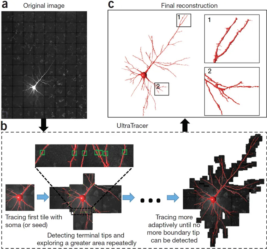
(a) 3D confocal image stack of a Lucifer-Yellow-labeled human pyramidal neuron. The voxel size is 0.18 × 0.18 × 0.5 μm, and the overlaid grid (black lines) indicates how the image volume is subdivided into uniform tiles. (b) UltraTracer first traces the subarea containing the soma and then detects the neuron terminal tips in the reconstruction, and adaptively explores and traces neighboring subareas. Green boxes indicate terminal tips detected in tracing a subarea. (c) Final reconstruction produced by UltraTracer, with zooms of two parts for detailed visualization.

The core algorithm of UltraTracer (Fig. 1) reconstructs a neuron structure from the available image data on the basis of a formulation of maximum-likelihood estimation. The underlying assumption is that the occurrence of a specific neuron structure could be modeled using the joint probability of all of its subparts given the image. Briefly, UltraTracer iteratively factorizes the joint probability based on progressive maximization of conditional probabilities of the occurrence of salient and continuous subparts of a neuron (Supplementary Note). Therefore, UltraTracer explores an image by following where the neurite signal goes, on the basis of either adaptive windows generated based on the already reconstructed neuron structure or certain domain knowledge (prior information or statistics) of neuron morphology, to help refine the choice of the next tracing subarea (Supplementary Note). This process repeats until the neuron structure grows as completely as possible. We designed the UltraTracer software to quickly extract an arbitrary subvolume of interest from large neuron image files (Supplementary Note), and thus smoothly traced an image archive without the need to load a large number of image voxels into computer memory.

As a crucial utility that was not previously available to reconstruct large-scale data sets, UltraTracer extends an arbitrary base tracer to make it possible to trace an ever-increasing image volume. We tested this by considering ten representative base tracing algorithms ported to BigNeuron³ (https://github.com/BigNeuron/BigNeuron-Wiki/wiki/Neuron-Reconstruction-Algorithms) that have different design principles, performances, and output formats (Supplementary Figs. 1, 2, and 3; Supplementary Note). The performance gain of UltraTracer over the direct use of certain base tracers was within the range of 3–6 times (Supplementary Fig. 1b). UltraTracer results were accurate, as their average spatial distances to independent manual reconstructions were around 3 voxels, comparable to the spatial distance of the manual reconstructions themselves (3.56 voxels) (Supplementary Fig. 1b). In addition, for two base tracers, NeuTube⁴ and MOST⁵, UltraTracer had a gain of 10–30-fold in tracing accuracy (Supplementary Fig. 1b). Testing of six other base tracers (Supplementary Fig. 2) indicated similar improvement. When a computer with smaller memory was used or the image volume increased greatly, UltraTracer was consistently superior to the conventional approach (Supplementary Fig. 3).

The APP2 algorithm⁶ was a good base tracer, in terms of speed–accuracy trade-off (Supplementary Fig. 1), for both laser-scanning and brightfield images (Supplementary Figs. 3,4,5,6,7). The APP2-based UltraTracer scaled robustly in tracing the sparse neuronal structures in images with 521 billion voxels, reducing the data volume in tracing between 3 and 40 times (Supplementary Fig. 3). Typically a bigger data-volume reduction rate was achieved for a larger image volume. Measured in terms of spatial distance, bifurcation points, and five other morphological and topological features, and compared against the statistics drawn from collections of reconstructions produced using control images (Supplementary Note), the accuracy of reconstructions produced by UltraTracer was consistent with that of reconstructions generated using the traditional approach when the image data set could be accommodated by the computer memory (Supplementary Fig. 3, bottom left).

We used UltraTracer to combine multiple different base tracers (Supplementary Note; Supplementary Figs. 8 and 9), for example using APP2 in the soma area while using NeuTube and MOST to trace curvilinear structures. In a more complicated case, for every adaptively searched image region, we profiled the reconstructions generated by several base tracers, and then chose either the best reconstruction or their consensus as the result from the current image region (Supplementary Fig. 9). In this way UltraTracer could provide more consistent reconstructions compared to manual work. We also used UltraTracer to reconstruct human neurons, including their axons and dendrites, from separate but serial slices of brain tissue (Supplementary Note; Supplementary Fig. 10). Additional information about the algorithm can be seen in Supplementary Figures 11,12,13.

Supplementary Material

SF1

Supplementary Figure 1 UltraTracer extends and improves various base tracers to reconstruct large image volumes.

A. UltraTracer with four base tracers APP1, APP2, NeuTube, and MOST (Supplementary Note) applied to image regions R1 and R2. B. Comparison of UltraTracer and the direct use of base tracers. TR: traditional method (i.e. using a base tracer directly to reconstruct the entire 3-D image volume); UT: UltraTracer; BASDM: Best Average Spatial Distance compared with Manual reconstructions; PM: Peak computer-Memory; TT: Tracing Time. The image volume used has 2111×3403×291 voxels. Two independent human manual reconstructions were used for comparison; their BASD (Best Average Spatial Distance) is 3.56 voxels.

SF2

Supplementary Figure 2 Comparison of UltraTracer and the direct use of 6 additional base tracers on a human neuron image stack.

These 6 base tracers including Snake (Narayanaswamy, et al, 2011), Minimum Spanning Tree (MST as used by a number of groups independently; the original idea could be referred as Dijkstra, 1959), NeuroGPSTree (Quan, et al, 2016), Rivulet (Liu, et al, 2016), TReMAP (Zhou, et al, 2016), and nctuTW(Lee, et al, 2012). Two base tracers, Snake and Rivulet, were not able to generate the reconstruction using TR, since their usage of computer-memory exceeded the available memory of the testing computer (128 GB). One base tracer, nctuTW, failed to generate the reconstruction using TR or UT because it was too slow (in fact, it could not even produce a reconstruction for a 768×768×291 voxel sub-volume of the human neuron image stack within three hours). The image stack is the same one used in Supplementary Figure 1B.

SF3

Supplementary Figure 3 UltraTracer (with base tracer APP2) is scalable with respect to ultra-volumes of neuron images, without compromising the tracing accuracy in terms of spatial distance, morphological and topological features.

TR: Traditional approach. UT: UltraTracer. Testing data: neurons 1, 2, 3, and 4 are confocal image stacks of human pyramidal neurons, neurons 5 and 7 are confocal image stacks of mouse pyramidal neurons, neuron 6 is a brightfield image stack of human pyramidal neuron. In reconstruction-consistency testing of TR and UT based on various features, the “percentage of structure difference” of two reconstructions measures the portion of their visible difference (the nearest matching reconstruction nodes in two tracings are more than 2-voxel apart), the “percentage of matched bifurcation pairs” is defined as the portion of reciprocally best matching bifurcation points divided by the average number of bifurcation points of two reconstructions, the “total length”, “total surface”, and “total volume” are the length, the surface, and the volume of all neuronal compartments in reconstructions, the “average diameter” is the average diameters of all compartments in a reconstruction, the “Hausdorff dimension” (Falconer, 2004) measures the fractal dimension of reconstructions. In parentheses, the statistics (mean +/− s.d.) derived from TR-reconstructions using 59 rotated images (every 6 degrees around the center of XY-plane) for each neuron are shown as controls. Bottom-right inset: Regression analysis of peak memory and tracing time versus the image volume tested on 31 brightfield images.

SF4

Supplementary Figure 4 Application of UltraTracer to brightfield imaging image stacks of mouse V1 neurons.

A. An example of brightfield image. B. Enhanced image using an adaptive approach (Zhou, et al, 2015). C. UltraTracer reconstruction based on the enhanced image in B. Different colors indicate reconstructions from different image regions.

SF5

Supplementary Figure 5 UltraTracer enhanced by incorporating prior knowledge of the adaptive subarea (window) size in tracing, which was learned from largescale statistics of mammalian neuron reconstructions.

A. The estimated window size (in x, y, and z) as a function of the distance of a neuron compartment to the soma. The maximum window size was set to be 1024 voxels. B. Comparison results of two tracings, one with the TDAW method (magenta) and another with PTDAW (green), where the prior is the estimated window size in A. In each zoom-in region (R1 ~ R3), the gray-scale image voxels are also displayed. The two reconstructions are slightly offset in x-direction for better visualization.

SF6

Supplementary Figure 6 Average neuron-compartment density as a function of the distance between the neuron-compartment and the soma.

This information was used as a look-up table for PTDAW to avoid potential skewed estimation based on any extreme cases.

SF7

Supplementary Figure 7 Tracing results of TDAW (magenta) and PTDAW (green) for a mouse pyramidal cell (voxel size 0.143μm×0.143μm×0.28μm).

Reconstructions are slightly offset in x-direction for better visibility.

SF8

Supplementary Figure 8 Combination scheme 1: UltraTracer combines different base tracers to achieve better performance on a 3-D confocal image stack of a Lucifer Yellow labeled human pyramidal neuron.

APP2+NeuTube: the soma region is traced by APP2, and the rest is traced by NeuTube. APP2+MOST: the soma region is traced by APP2, and the rest is traced by MOST. APP2+NeuTube explores 2.80 billion voxels areas, but needs 2158.69s for tracing. APP2+MOST generates a relatively complete reconstruction (1.90 billion voxels scanned areas) with a much faster tracing speed (89.18s tracing time). Neuron data used here is the neuron 4 in Supplementary Figure 3.

SF9

Supplementary Figure 9 Combination scheme 2: UltraTracer real-time selects suitable tracing algorithm on a confocal image stack of human pyramidal neuron.

For each explored image region, two reconstructions (APP2 and NeuTube) were generated first. For the “best candidate” result, the contrast-to-background ratio in the image region around the reconstruction was used to choose the suitable algorithm. For the “consensus” result, the union of two reconstructions is used as the result for the current image region. Both two real-time selection results had similar BASDM scores (2.62 voxels and 3.42 voxels in the best candidate result, and 3.73 voxels and 4.18 voxels in the consensus result) to APP2 (2.78 voxels and 3.57 voxels) and NeuTube (5.17 voxels and 5.42 voxels). Neuron data used is the same neuron in Supplementary Figure 1B.

SF10

Supplementary Figure 10 An application example of UltraTracer for tracing multiple biocytin-filled human neurons with axons.

The images were from 3 sections, each of which was imaged separately (voxel size 0.114μm×0.114μm× 0.28μm). UltraTracer was used to reconstruct automatically based on multiple starting locations on these separate image stacks. The final reconstruction (red) was assembled using the NeuronAssembler tool in Vaa3D (vaa3d.org). The reconstruction, including axons and dendrites, was also manually validated (blue in zoom-in views, slightly offset in x-direction for better visibility), with some substructures of the reconstruction edited (addition or deletion of some structures based on visual inspection). Overall more than 90% portion of the automatic reconstruction could be easily validated manually for this example, while the 10% were too difficult even for manual reconstruction (e.g. the manual deletion in location d of region R1 seemed to be a problematic deletion in the manual correction). The total lengths of the automatic and manually curated reconstructions were 22.51 and 20.15 mm, respectively.

SF11

Supplementary Figure 11 UltraTracer workflow.

SF12

Supplementary Figure 12 Fixed versus adaptive tile size.

A. Based on the boundary tips of the left tile (containing the soma), three image tiles (1.1 billion voxels) have been loaded to trace the right side of the neuron with fixed tile size. B. A much smaller part (0.55 billion voxels) of the image volume has been loaded with the adaptive tile size. The purpose of this figure is to show the comparison of loading areas to trace the right side of the neuron using fixed and adaptive tile sizes. So only the part of the traced neuron structures is shown.

SF13

Supplementary Figure 13 One reconstruction fusion example.

A. Over-tracing due to overlap between adjacent tiles. B. The over-tracing error has been fixed.

References

- 1.Helmstaedter M Nat. Methods 10, 501–507 (2013). [DOI] [PubMed] [Google Scholar]
- 2.Acciai L, Soda P & Iannello G Neuroinformatics 4, 353–367 (2016). [DOI] [PubMed] [Google Scholar]
- 3.Peng H et al. Neuron 87, 252–256 (2015). [DOI] [PMC free article] [PubMed] [Google Scholar]
- 4.Zhao T et al. Neuroinformatics 9, 247–261 (2011). [DOI] [PMC free article] [PubMed] [Google Scholar]
- 5.Wu J et al. Neuroimage 87, 199–208 (2014). [DOI] [PubMed] [Google Scholar]
- 6.Xiao H & Peng H Bioinformatics 29, 1448–1454 (2013). [DOI] [PMC free article] [PubMed] [Google Scholar]
Associated Data
This section collects any data citations, data availability statements, or supplementary materials included in this article.
Supplementary Materials