

Abstract
The premise of this report is that functional Near Infrared Spectroscopy (fNIRS) imaging data contain valuable physiological information that can be extracted by using analysis techniques that simultaneously consider the components of the measured hemodynamic response [i.e., levels of oxygenated, deoxygenated and total hemoglobin (oxyHb, deoxyHb and totalHb, respectively)]. We present an algorithm for examining the spatiotemporal co-variations among the Hb components, and apply it to data obtained from a demonstrational study that employed a well-established visual stimulation paradigm: a contrast-reversing checkerboard. Our results indicate that the proposed method can identify regions of tissue that participate in the hemodynamic response to neuronal activation, but are distinct from the areas identified by conventional analyses of the oxyHb, deoxyHb and totalHb data. A discussion is provided that compares these findings to other recent studies using fNIRS techniques.
I. Introduction
Since its original adaptation into a tomographic imaging method (Barbour, Graber et al. 1990; Aronson, Barbour et al. 1991), functional near infrared spectroscopy (fNIRS) has found an expanding range of applications, with a particularly important area being the study of event-related neuroactivation of the cerebral cortex (Villringer and Chance 1997). Enabling these studies is the fact that light in the near infrared wavelength region can penetrate through bone and soft tissue, allowing for detection of photons that have propagated over distances of several centimeters. These measures can be used to track temporal variations in the hemoglobin (Hb) signal as a surrogate marker for neuroactivation, in a manner similar to the Blood Oxygenation Level Dependent (BOLD) signal used in functional Magnetic Resonance Imaging (fMRI) studies. However, unlike the BOLD signal, which is principally sensitive to variations in the level of deoxyhemoglobin (deoxyHb), the NIRS signal is able to independently measure the concentrations of oxyhemoglobin (oxyHb) and deoxyHb, thereby allowing for differentiation between changes in deoxyHb associated with variations in Hb oxygen saturation and in blood volume.
A common practical aim of both fMRI and fNIRS investigations is to understand where in the brain neural events are occurring. In principle, the independent observation of oxyHb and deoxyHb should allow for a richer characterization of the underlying mechanisms governing neural activation than the BOLD signal allows. However, the methodological tool-set available to study fNIRS phenomena is currently not nearly as rich as that available to the fMRI community (Cox 1996). In the case of NIRS, this has led to studies that have been largely observational, assessing predominantly individual-subject responses to stimulation rather than attempting to generalize these to a group of subjects. As experience has shown in other fields, in order to move beyond this level of inquiry and to allow for inferences about group characteristics, it is necessary to: 1) ascertain which aspects of the surrogate marker are most suitable for detecting (i.e., most representative of) the signal of interest (in this case, the spatial and temporal features of neural activation), 2) ascertain which aspects of the signal are most reliable, and 3) to adopt statistical methods appropriate for group inferences.
Invariably, effective pursuit of the preceding goals relies critically on having access to appropriate tool-sets, along with sufficient experience with the associated methodologies to ascertain their practical limits. In an effort to address some of these concerns, in previous studies, Barbour and colleagues have outlined a novel methodological framework that has the potential to support a much broader understanding of the information content of the NIRS signal (Barbour 2007; Barbour, Pei et al. 2007), and have implemented new capabilities that assess the accuracy of functional NIRS studies with the aid of programmable phantoms (Barbour, Ansari et al. 2008).
In this report, we focused on exploring the potential utility of the novel framework (Barbour 2007; Barbour, Pei et al. 2007), within the context of a simple visual activation study. Central to this approach is the expectation that elements of the Hb signal will co-vary in ways that can reveal information regarding the underlying phenomenon of tissue-vascular coupling. While this relationship is generally well appreciated, methods that make direct use of the co-variations among the elements of the Hb signal have been lacking. More common are strategies that either examine the Hb components individually, or that consider them simultaneously but for the purpose of extracting an individual signal that, a priori, is assumed independent of other sources of spatiotemporal variability that are coincident with the neuroactivation. In particular, we have explored the spatial and temporal components of these co-variations that are associated with neuroactivation induced by a visual stimulus. Among the findings is evidence that regions of activation identified by this approach may differ from those derived from analysis of individual elements of the hemoglobin signal.
II. Experimental Methods
1. Subjects
Ten right-handed, healthy adults (8 men), with a mean age of 27.6 years old (range: 22–36 years) were recruited from the community. Exclusionary criteria were a history of neurological disease, psychiatric disorders, or alcohol or drug use disorders. The data from one subject (male) was unusable due to elevated noise levels caused by instability in contact and was therefore not included in the group analyses.
2. Data Collection
a. Apparatus
A multi-channel, continuous wave, near-infrared tomographic imager (DYNOT Imaging System, Model 264, NIRx Medical Technologies LLC, Glen Head, NY 11545) was used to obtain measures of temporal variations in the tissue concentrations of oxyHb, deoxyHb and totalHb. Data collection was based on a time-multiplexing scheme wherein light from two optical laser diode sources, operating at 760 and 830 nm, is simultaneously directed to the tissue through 3-mm diameter bundles of glass optical fibers (diameter of the individual glass filaments in the bundle was 50 μm) (Schmitz, Löcker et al. 2002). Using a fast optical switch, a 30-element array can be scanned at a framing rate of approximately 2 Hz. Here, we used an array having a 3×10 arrangement of optical fibers, with 1 cm spacing between adjacent optodes, positioned symmetrically about the mid-line over occipital scalp. Illuminating and detected light were conducted between the imager and head via bifurcated optical fibers, 3 m (10 ft) in length, that had a common end and served to both transmit and receive optical signals. Individual legs of the fiber bundle were fitted to the optical switch (transmitter leg) and to the detector unit (receiver leg). The common end was housed within an open scaffolding helmet forming an attached tether of optodes that are spring loaded to facilitate good contact with the scalp (Barbour, Graber et al. 2004). Added mechanical support was achieved by using a multi-axis articulating arm containing a strain relief that allowed for off-loading of the weight of the optical fibers. Participants were seated in a comfortable chair while performing the experiment. The adjustable helmet was individually fitted to ensure the optodes were comfortable and remained stationary on the scalp.
b. Light Detection
Parallel sampling of light intensities from the optode array was performed using sample–and-hold techniques. Discrimination of light intensities from the different laser sources was achieved by amplitude-modulating the sources in the audio-frequency range (frequency encoding) and referencing the resulting signal to DC. To support simultaneous optical measurements from detectors located multiple distances from any one source, a gain-switching scheme was used that updated with each new source position. In combination, this allowed for dense sampling of optical signals over a distance ranging from 0 (i.e., source and detector were co-located) to 5 cm from any source. The number of data channels was the product of the number of sources and number of detectors (i.e., 30S × 30D = 900 S–D pairs). In practice, however, the number of usable SD-pairs was less than this because some pairs exceed the maximum sensing distance.
c. Stimuli
On each trial, a reversing circular checkerboard stimulus (see Figure 1; radius = 60 mm, visual angle = 9.5°, reversal rate = 8 Hz) was presented at fixation for 2 seconds. The black and white checks were scaled linearly with eccentricity, and were presented on a gray background with the same mean luminance as the checkerboard. Thereafter, an inter-trial interval ensued that ranged (randomly) from 11 to 20 seconds, in one second intervals. Subjects were asked to maintain fixation throughout. 120 trials were presented.
Figure 1.
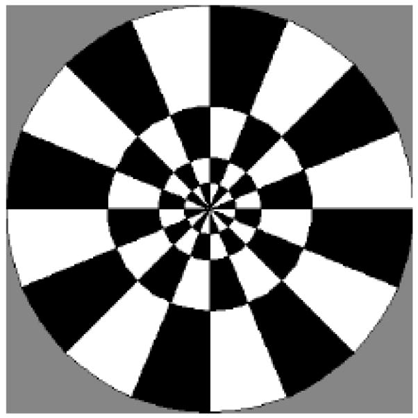
The contrast-reversing checkerboard pattern used to evoke a visual response.
d. Procedure
After obtaining informed consent in accordance with the Institutional Review Board at the Kessler Foundation Research Center, and ensuring that the exclusion criteria were not met, subjects were seated in a comfortable chair. The 10×3 array of NIRS optodes was positioned over the back of the head, using the inion as a landmark: the bottom of the array was placed immediately above the inion, and the array was centered on the subject’s head (i.e., 5 columns of optodes to the right of the midline, 5 to the left). After ensuring good contact between the optodes and the scalp, and that they were receiving sufficient signal, the experiment commenced. The florescent overhead lights were turned off, and 5 min of baseline activity was recorded with the subject’s eyes closed. After this baseline period, a laptop computer (HP/Compaq nw8240) was placed at a comfortable viewing distance (approximately 30 cm) in front of the subject, on a table over his/her lap. Stimulus presentation was controlled by the Presentation software package [http://www.neurobs.com/]. After the spacebar was pressed on the laptop, a countdown (3, 2, 1) readied the subject for the first stimulus. Each time a stimulus was presented on the laptop, the stimulus-delivery software generated a transistor-transistor logic (TTL) pulse that was sent to the imager, which logged when each stimulus was presented in terms of acquisition number. This information served to time-stamp each stimulus presentation allowing for the construction of a stimulation time series which was used in the deconvolution of the data.
III. Data Analysis
A. Preprocessing
Data pre-processing began with the use of the Near-infrared Analysis, Visualization and Imaging (NAVI) software package (NIRx Medical Technologies LLC., Glen Head, NY 11545) (Pei, Wang et al. 2006). The raw data was low-pass filtered to exclude the cardiac frequency (0.8 Hz cutoff) and subjected to a noise threshold of coefficient-of-variation (CV) < 25%, for both illumination wavelengths, during the baseline period. An additional criteria imposed was to limit inclusion of detectors having a maximum distance of 4–5 cm. In practice this had the effect of imposing an upper limit of noise in the data that varied from 5–25% depending on the subject. The higher threshold represents an amount of variability that is approximately twice that of naturally occurring vascular rhythms (Fabbri, Henry et al. 2003; Boas, Dale et al. 2004). Corrections for small variations in laser power and coupling efficiency of the optical switch were made by dividing each detector time series by the time series for the detector co-located with the source optode.
B. Image Recovery
3D image time series of the wavelength-dependent absorption coefficient (μa) were computed using the Normalized Difference Method of Pei et al. (Pei, Graber et al. 2001), applied to a segmented finite-element-method (FEM) mesh computed from a MR map of an adult male using the EMSE software suite (http://www.sourcesignal.com). The same MR map was employed for purposes of registering optical findings onto underlying tissue structures revealed by the selected atlas. It should be noted that, whereas there is agreement between the MR model used for registration and that from which the image-reconstruction operator was computed, no specific effort has been made to compensate for any variance in image findings that may arise from differences among the subjects’ head shapes, or from small differences in optode placement.
The linear image recovery problem was numerically solved by using a truncated SVD method, where the number of singular vectors retained was sufficient to account for 98% of the cumulative sum of all singular values (this was subject-dependent because the number of data channels rejected differed across subjects). Dual-wavelength μa values were transformed to changes in the concentration of oxyHb and deoxyHb a 2×2 system of linear equations (Choi, Wolf et al. 2004). The associated image map was subsequently converted into ANALYZE format and exported (voxel size = 2.75×3.3×2.75 mm3 in the X Y and Z directions respectively) to allow for additional processing using the AFNI image analysis suite (Cox 1996).
For simplicity, the identified individual tissue regions were assigned uniform values of μa = 0.06 cm−1 and μs = 10 cm−1, at both illuminating wavelengths. These values correspond to a mean oxygenation level of 68.8% and a total Hb concentration of 29.3 μM. The former value coincides well with published reports of mixed venous oxygenation values for the adult brain (Yoshitani, Kawaguchi et al. 2005). We are aware that the latter value underestimates the hemoglobin content for gray matter by nearly a factor of three (Zheng 2008). We nevertheless have chosen to use this reduced value in an effort to improve the numerical stability of computed results and to minimize known spatial biases associated with first-order reconstructions obtained from back-reflection studies (i.e., reconstructed image features are biased towards the surface) (Boas, Dale et al. 2004). Use of a lower background absorption value reduces the intensity gradients in the medium. This has the effect of enabling more accurate computation of light intensities within the medium while using a lower-density 3D FEM mesh. Thus we retain relative accuracy in the computed light intensities while maintaining a reasonable computational effort. We have also found that the known biasing of reconstruction results towards the surface, associated with back-reflection measurements, is less if a lower background absorption value is employed. This is expected, as the lower absorption value will force the reconstruction to greater depths. Thus we have empirically found that the background absorption value used here represents a good compromise between solution stability and factors impacting on the reconstruction accuracy.
Use of a linear image-reconstruction operator is a source of additional amplitude bias (underestimation) in the computed μa values. A reasonable correction to this bias can be derived by introducing variations in absorption to the MR-based head models that correspond to amplitudes derived from experiment, and comparing recovered values to true values. In the case of the region of maximum activation (see Figure 4), the correction factor obtained was 240. With this correction, we find that amplitude of the Hb response to neuroactivation is on the order of 0.38 μM, a value similar to other reports (Zeff, White et al. 2007).
Figure 4.

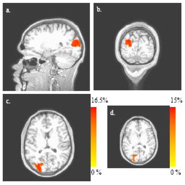
4(a)–(c): Three orthogonal views (sagittal, coronal and axial, respectively) of the oxyHb response to visual stimulation, as determined from a single Hb-component analysis (area under curve) across all nine participants (corrected significance level of α = 0.05). In (e) and (f) the axial views of the deoxyHB response and totalHb response are shown, respectively. Curves plotted in 4(d) show the fitted response for all Hb components, for one the nine participants, at the voxel with the largest response at the group level [(X,Y,Z) = (18, −103, −12)].
Reconstruction results were obtained using a 3D FEM mesh consisting of 2,400 nodes (10,371 elements), had an external (scalp) surface area of approximately 65 cm2, and a maximum depth of 3 cm from the external surface. (A surface view of this mesh, with the 30 optode locations indicated, is shown in Figure 2.)
Figure 2.
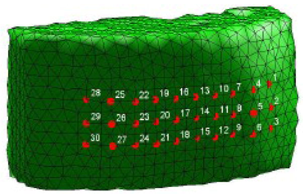
Exterior view of the FEM mesh used for image reconstruction, with the positions of the 30 source/detector optodes indicated.
C. Data Post-Processing
Using AFNI, totalHb was calculated by adding the oxyHb and deoxyHb time series. The oxyHb, deoxyHb and totalHb data were then analyzed in the following ways.
1. Single Hb-Component Analysis
A deconvolution algorithm was used to calculate the best-fitting gamma-variate function for the visual stimulus at each voxel (time resolution: 0.526 sec) [http://afni.nimh.nih.gov/afni/doc/manual/3dDeconvolve], which represents the hemodynamic response function (HRF). A nonlinear regression program (Garavan, Ross et al. 1999) was then used to quantify the event-related activation by finding the area under the gamma-variate curve (described in Garavan, Ross et al. 1999). To compare the area under the curve across participants (i.e., a random effects analysis), a t-test was performed, for each image voxel individually, using a corrected threshold of 0.05 (individual voxel significance level: α = 0.01; cluster size (see below): 54 voxels). This provided a statistical test of the goodness-of-fit between the experimental manipulation and changes in oxyHb, deoxyHb and totalHb, using standard techniques that have been developed for the analysis of fMRI data.
The correction for multiple comparisons was achieved by imposing a cluster-level threshold (i.e., a minimum number of voxels in any given cluster of activation) as well as a voxel-level probability threshold. The cluster-level threshold, found using Monte Carlo simulations [AlphaSim: http://afni.nimh.nih.gov/afni/doc/manual/AlphaSim], was 54 contiguous voxels.
2. Combinatorial-States (Multiple Hb Components) Analysis
a. Definitions of Combinatorial States
At any given time frame and image pixel, the instantaneous levels of all Hb components (oxyHb, deoxyHb and totalHb) are either greater than or less than their respective baseline temporal mean values. As indicated in Table 1, a straightforward non-parametric index of co-variability among the three components can be defined by assigning a different label to each permutation of algebraic signs of the differences between instantaneous and baseline-mean levels. (While eight permutations of signs are mathematically conceivable, only the six included in Table 1 are physically possible.) Associated with each defined state is a tentative physiological interpretation (see Discussion) reflecting the rationale that underlay the development of the combinatorial approach: for example, given the information that tissue in a specified location is in a state of uncompensated O2 debt, we could expect to find that the deoxyHb level there is elevated, while the oxyHb and totalHb levels are reduced relative to their baseline mean values. It should be noted, however, that the practical utility of the combinatorial states is not contingent upon universal validity of the physiological correlates indicated in Table 1.
Table 1.
Definitions of the combinatorial states. Tentative physiological correlates are indicated.
| State 1 | State 2 | State 3 | State 4 | State 5 | State 6 | |
|---|---|---|---|---|---|---|
| oxyHb | − | − | − | + | + | + |
| deoxyHb | − | + | + | + | − | − |
| totalHb | − | − | + | + | + | − |
| Balanced | Uncompensated O2 debt | Compensated O2 debt | Balanced | Uncompensated O2 excess | Compensated O2 excess |
Two methods for extracting physiological information from the states (among others that have been explored (see Discussion)) were applied to the data collected in the study reported here. Both make use of the theoretical expectation that, under baseline conditions, one would expect to find equal numbers of image voxels in, for example, State 1 and in State 4 at any given time frame, and would expect to find a given voxel in State 1 and State 4 for equal amounts of time. The same expectations hold for the following pairings of states: 2 and 5, 3 and 6, 2+3 (i.e., the voxel is in either State 2 or State 3) and 5+6, 1+2+3 and 4+5+6, 1+2+6 and 3+4+5, and 1+5+6 and 2+3+4.
b. Time-Fraction Measures
For each voxel, the HRFs for oxyHb, deoxyHb and totalHb were used to compute the fraction of time spent in each of the six states defined in Table 1, over the 20 seconds following stimulus presentation. This was accomplished by counting the number of time frames for which a particular state (e.g., State 4) was assigned to the voxel, and dividing by the total number of time frames (i.e., 38) in the 20-s post-stimulus interval. Following this, for each subject and image voxel separately, differences were computed between the time fractions for all state pairings expected to have equal time fractions under baseline conditions. Then, for each image voxel and state pairing separately, t-tests across all nine subjects were performed to determine which paired differences were significantly different from zero. The same correction for multiple comparisons as described for the single-component analyses was applied here.
c. Volume-Fraction Measures
The purpose of this analysis was to determine what fraction of a region of interest (ROI) is in a given state at each time frame. Because the experimental paradigm was designed to evoke a response principally in the primary visual cortex, only the data within a spherical ROI (radius = 20 mm; volume = 1,137 voxels), centered in the lateral dimension on the calcarine sulcus, was included in this analysis. This ROI (see Figure 3) was large enough to include the entire calcarine fissure in the rostro-caudal dimension.
Figure 3.
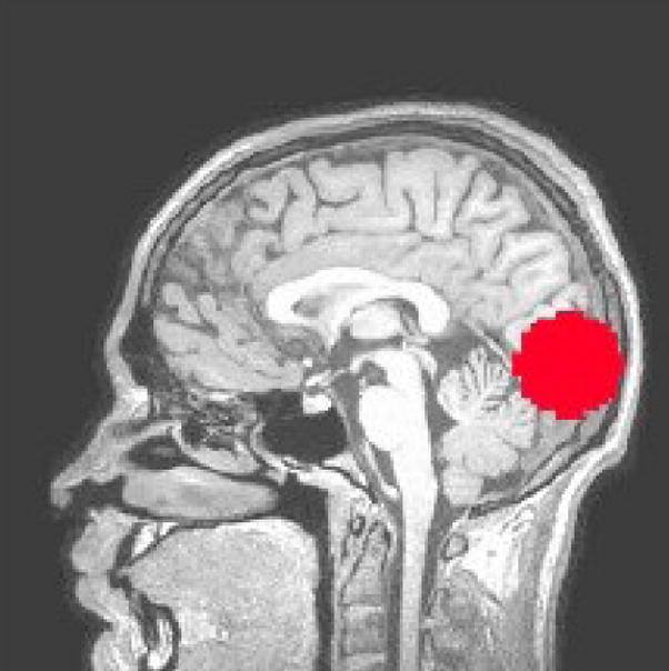
The Region of Interest (ROI) used to compute partial-volume measures.
For each time frame of the 20-s interval following stimulus presentation, the HRFs for oxyHb, deoxyHb and totalHb were used to compute the fraction of the ROI that was in each of the six states defined in Table 1. This was accomplished by counting the number of voxels that had a particular state assigned (e.g., State 4), and dividing by the total number of voxels in the ROI. Following this, for each subject and time frame separately, differences were computed between the volume fractions for all state pairings expected to have equal volume fractions under baseline conditions. Then, for each time frame and state pairing separately, t-tests across all nine subjects were performed to determine which paired differences were significantly different from zero (individual-test significance level: α = 0.05). As a correction for multiple comparisons, we required that a statistically significant difference be seen at three or more consecutive time frames, having found through Monte Carlo simulations that the chance probability of this occurrence is < 0.005 for the number of t-tests carried out (7 state pairings × 38 time frames = 266 tests; the low-pass filter cutoff frequency was sufficiently high that no additional allowance is needed for temporal autocorrelation between consecutive time frames).
The same computations were carried out over the 600 baseline time frames, using the reconstructed deoxyHb, oxyHb and totalHb data directly, in order to test the theoretical expectations (e.g., State 1 volume fraction = State 4 volume fraction) described above.
IV. RESULTS
A. Single Hb-Component Analysis
Figure 4 shows regions of activation in response to the visual stimulus that were identified by the area-under-curve analysis described above (III.C.1). Figure 4(a)–(c) (oxyHb data) shows three orthogonal sections that intersect in the voxel with the largest area under the curve. For the results for deoxyHb [Fig. 4(e)] and totalHb [Fig. 4(f)] are also shown, demonstrating the similarity among the regions identified for each component (only the axial slice is shown, but the sagittal and coronal views were substantially very similar to that seen in the analysis of the oxyHb data. Inspection of the spatial maps reveals that many of the identified voxels are localized to the visual cortex, but that there are some regions of activation outside of it. Figure 4(d) shows single-subject data of the estimated HRF for oxyHb, deoxyHb, and totalHb.
The size and approximate anatomical locations of the statistically significant regions, for all three Hb-components, are reported in Table 2. See that the volume of activation varies over a range of 8–15 cm3, having a sensitivity trend of oxyHb> totalHb > deoxyHb. It is important to note that while the data here represent a good estimate of the location of oxyHb, deoxyHb and totalHb area, it is only an estimate. The spatial resolution of NIRS is in the order of cm, and the precise anatomy of each subject (e.g., MRI scans) was not available.
Table 2.
Summary of statistically significant results from the single Hb-component random effects analyses.
| Hb Component | Number of Voxels/Volume (cm3) | X Y Z Coordinates (mm) | t-statistic | Approximate Anatomical Location |
|---|---|---|---|---|
| oxyHb | 587/14.6 | −18 −103 −3 | 4.19 | Cuneus/Lingual Gyrus (BA18) |
| deoxyHb | 321/8.0 | −18 −103 −3 | 4.55 | Cuneus/Lingual Gyrus (BA18) |
| totalHb | 455/11.4 | −15 −103 −3 | 3.19 | Cuneus/Lingual Gyrus (BA18) |
B. Combinatorial-States (Multiple Hb Components) Analysis
Here we explored the extent to which examination of the co-variations among the different Hb components can reveal information qualitatively distinct from that obtainable from the conventional, single-component analysis. This was accomplished by computing the position-dependent time fraction and time-dependent volume fraction for each of the six combinatorial states and subjecting them to the same type of statistical analysis as in the preceding section. It should be noted that time fractions can identify where vascular phenomena related to neuroactivation occur, but not when. The complementary volume fractions convey information about when activation occurs in the volume considered, but not where.
1. Time-Fraction Measures
Two types of comparisons may be indicative of a vascular response associated with neuroactivation: 1) the fraction of time that a voxel spends in a given combinatorial state during the post-stimulus time interval, compared to the fraction of time spent in the same state during the baseline; 2) the difference, during the post-stimulus interval, between the fractions of time that a voxel spends in two states (or two combinations of states) that are expected to have zero time-fraction difference under baseline conditions. As indicated in Table 3, comparisons of the first type failed to yield statistical significance. This is perhaps unsurprising given that the subjects were not asked to maintain fixation during that interval. Comparisons of the second type achieved statistical significance (paired t-test), for three states-pairings that are related to the difference between the fractions of time that voxels spend in states of O2 debt and O2 excess. Spatial maps showing which voxels participate in the statistically significant differences, for two comparisons of the second type, are presented in Figure 5.
Table 3.
Summary of statistically significant results from the combinatorial-state time-fraction random effects analyses.
| Comparison | Number of Voxels/Volume (cm3) | X Y Z Coordinates (mm) | t-statistic | Approximate Anatomical Location |
|---|---|---|---|---|
| State 2 vs. State 5 | 176/4.4 | −21 −100 5 | 4.16 | Cuneus/Middle Occipital Gyrus (BA18) |
| States (2+3) vs. State (5+6) | 357/8.9 | −26 −83 19 | 9.2 | Middle Occipital Gyrus (BA18) |
| States (1+2+3) vs. State (4+5+6) | 62/1.5 | −26 −80 16 | 3.54 | Middle Occipital Gyrus (BA19) |
Figure 5.
5(a)–(c): Difference between the fractions of the 20-s post-stimulus time interval that image voxels spend in State 2+3 (i.e., either State 2 or State 3) and State 5+6 (maximal difference = 16.1%). Three orthogonal views (sagittal, coronal and axial, respectively) of the time-fraction response to visual stimulation are shown (corrected significance level of α = 0.05). The axial view for the time-fraction difference between State 2 and State 5 is shown in Fig. 5(d) (maximal difference = 14.5%).
It is noteworthy that all of the statistically significant regions listed in Table 3 show little spatial overlap with the volumes of activation identified on the basis of the magnitude of the hemodynamic response (Table 2, Fig. 4). This is mathematically plausible, as the combinatorial-state definitions deliberately make use of only the algebraic signs of the Hb levels, and it offers a suggestion that the different approaches to analysis of fNIRS data reveal different aspects of the overall vascular response to neuroactivation.
An additional interesting feature of the results shown in Fig. 5 is that every voxel in the statistically significant volume has the same, positive, algebraic sign for the difference between the State-2 and State-5 time fractions [Fig. 5(d)] or between the States-(2+3) and States-(5+6) time fractions [Fig. 5(a)–(c)]. That is, the entire region spends a larger fraction of the post-stimulus time interval in an O2-debt condition than in an O2-excess condition (according to the system in Table 1). This pattern is the opposite of the classical (positive) BOLD response, a finding that has been reported in the fMRI literature (Bressler, Spotswood et al. 2007) While voxels exhibiting the complementary (i.e., more time spent in O2-excess states than in O2-debt ones) behavior also should be present in the image volume (as suggested by results in the following section), they will not be revealed in the time-fraction analysis carried out here if they have a more diffuse spatial distribution and do not occur in clusters of at least 54 contiguous voxels.
2. Volume-Fraction Measures
The same two types of comparison as outlined in the preceding section can, in principle, be performed for the volume-fraction data. Here again, however, the absence of maintained fixation during baseline results in large inter-subject variances for those time intervals. Accordingly, only results for comparisons between different states within the post-stimulus time interval are presented here. Shown in Figure 6 are plots of the group-mean difference (solid curves) between the volume fractions for State 2 and State 5 [Fig. 6(a)], States 2+3 (i.e., O2-debt states) and 5+6 (i.e., O2-excess states) [Fig. 6(b)], States 1+2+3 (i.e., oxyHb levels lower than the baseline temporal mean value) and States 4+5+6 (i.e., elevated oxyHb levels) [Fig. 6(c)], and States 1+5+6 (i.e., deoxyHb levels reduced) and States 2+3+4 (i.e., elevated deoxyHb levels) [Fig. 6(d)]. The dashed curves indicate the mean ± one standard error, and asterisks indicate those time frames for which the group-mean difference is significantly different from zero; all but one of the labeled sub-intervals satisfy the multiple-comparisons correction of at least three consecutive significant time frames.
Figure 6.

Group-mean difference (solid curves) ± one standard error (dashed curves), between the volume fractions for different pairings of combinatorial states, during the 20-s post-stimulus time interval. 6(a): difference between the volume fractions for State 2 and State 5. 6(b): difference between the volume fractions for O2-debt states (2 and 3) and O2-excess states (5 and 6). 6(c): difference between the volume fractions for decreased-oxyHb states (1, 2 and 3) and elevated-oxyHb states (4, 5 and 6). 6(d): difference between the volume fractions for decreased-deoxyHb states (1, 5 and 6) and elevated-deoxyHb states (2, 3 and 4). Asterisk symbols indicate time frames for which the group-mean difference is significantly different from zero; significance corrected for multiple comparisons is present whenever three or more consecutive time frames are labeled. Dot-dash lines are the time-averaged (600 time frames) group-mean volume-fraction difference for the baseline time interval; dotted lines are the mean ± one standard error. Plus-sign symbols indicate time frames for which the post-stimulus |t|-score is greater than that for the baseline time interval; significance corrected for multiple comparisons is present whenever ten or more consecutive time frames are labeled.
Also indicated in Fig. 6 are the time-averaged volume-fraction difference computed for the baseline time interval (dot-dashed horizontal line) ± one standard error (dotted horizontal lines). The baseline group-mean differences all are very small. That is, even though the baseline volume fraction for State 2, for example, is highly variable across subjects, the volume fractions for States 2 and 5 are nearly equal, as predicted (III.C.2.a). The plus-sign symbols in Fig. 6 indicate those time frames for which the post-stimulus volume-fraction differences is more significant (i.e., larger t-score (absolute value)) than the corresponding baseline difference. We have conducted a probability-theory analysis showing that this phenomenon is statistically significant if it occurs at ten or more consecutive time frames, under the null hypothesis that the true volume-fraction differences are the same during the post-stimulus and baseline time intervals. The ten-or-more criterion is satisfied in two sub-intervals of Fig. 6(a)–(c). In particular, for the clusters of 11–21 consecutive time frames indicated in Fig. 6(a)–(c), the probabilities of chance occurrence range from 0.014 to 8.6×10⁻⁶.
The complementary shapes of the curves in Fig. 6(c) and 6(d) are consistent with the occurrence of a BOLD-like response following neuroactivation. We can probe the oxyHb (for example) component of the hemodynamic response by examining Fig. 6(c), 6(b) and 6(a) in turn, which effectively is sub-dividing the overall response into successively finer levels of resolution. This reveals, for these particular results, that the difference between the State 2 and State 5 volume fractions [Fig. 6(c)] is the principal determinant of the difference between the lowered-oxyHb and elevated-oxyHb volume fractions [Fig. 6(a)]. The temporal correlation that is evident by visual inspection of Fig. 6(a) and Fig. 6(c) is substantially greater than the correlations between the latter result and the time courses (not shown) for the volume-fraction differences between State 1 and State 4, and between State 3 and State 6.
The results in Fig. 6 contain both statistically significant positive and negative volume fraction differences; that is, at some time frames there is more State 2 than State 5 present, and at others there is more State 5 than State 2. This observation is consistent with our expectations for a hemodynamic response to neuroactivation, but may appear to conflict with the time-fraction results of the preceding section, where the entire statistically significant region had the same algebraic sign for the time-fraction difference. Also noteworthy is that there is little spatial overlap between the regions identified by the time-fraction analysis and the spherical ROI (see Fig. 3) used for the volume-fraction analysis. This apparent disparity, which may be re-visited in future studies, can be attributed to either, or both, of two likely phenomena. First is the requirement, which applies to the time-fraction analysis but not in the volume-fraction case, that the statistical significance be found in at least 54 contiguous voxels. Second, individual voxels participating in the Fig. 6(a) volume-fraction response may be in State 5 for many consecutive time frames during the first half of the hemodynamic response, and in State 2 for many consecutive time frames during the second half, while the numbers of State-2 and State-5 time frames are approximately equal. Hence, there would not be significant time-fraction difference.
Discussion
i. Summary of experimental findings
The data presented here replicate and extend the work of other researchers. We find robust activation of the visual cortex in response to a reversing checkerboard stimulus, as one would expect. This is evident in the analyses of the single Hb components (oxyHb, deoxyHb and totalHb). Moreover, the response for each of these components largely overlaps with the other two. This is similar to previous research (e.g., Toronov, Zhang et al. 2007). However, we have also extended what others have shown through a careful analysis of the combinatorial-states analyses (time-fraction and volume fraction of the six states). These data show that a significant region of tissue spends more time in O2 debt (State 2) than O2 excess (State 5; see Figure 5). In the context of fMRI, such an increase in O2 debt would correspond to a decrease in the BOLD response, and it is worth pointing out that such decreases in the BOLD response, in paradigms similar to this one, are not uncommon (e.g., Bressler, Spotswood et al. 2007). Turning to the volume fraction results, which were confined to an ROI in primary visual cortex, we find a pattern of results similar to what is frequently reported in the fMRI literature: an initial hyperemia (greater fraction of State 5) followed by a period of relative O2 debt (State 2), (Figure 6(a–c)). These data also showed a period of decreased deoxyHb, followed by a period in which deoxyHb levels rise (Figure 6(d)). (It will be recalled that that the quantity plotted in Fig. 6(d) is proportional to the difference between the number of voxels with below-average deoxyHb levels and the number of voxels with elevated deoxyHb levels.)
ii. Comparison of experimental findings to recent NIRS studies
Recently, several groups have published results regarding the response of the visual cortex to visual stimuli using methods that include NIRS techniques. Explicit comparison of these findings to the current study is difficult because of differences in measurement details, experimental protocol and approach to data analysis. Nevertheless some comparisons can be made. For instance, Toronov et al (2007), using a block design, explored the NIRS response using a stimulus with fixed contrast (100%) but with varying frequency (1–6 Hz). Similar to the results reported here, they found evidence of differential response activation depending on hemoglobin components and the size of the effected volume. They reported an activation volume that varied between 10–27 cm3 depending on Hb component in the order of oxyHb>deoxyHb>totalHb. We observed activation volumes of 8–15 cm3 depending on Hb component. The order of sensitivity we observed was oxyHb>totalHb>deoxyHb (Table 2). Also similar is the suggestion of a left-sided bias in the activation profile.
Rovati et al (2007) adopted a block design and an 8 Hz presentation rate, but varied the target contrast (1, 10, 100%). These researchers concurrently recorded electroencephalography (EEG) from the occipital cortex. They observed that both EEG and NIRS exhibit a titratable, linear response. Further evidence for differential sensitivities between the NIRS and EEG signals comes from a recent report by Herrmann et al (2008). The focus of this study was to explore the response of the visual cortex to emotional stimuli. These authors reported that while both techniques could distinguish positive and negative stimuli from neutral, the discriminatory power of the NIRS method was more evident for deoxyhemoglobin than for oxyhemoglobin. Given that the resting mixed –venous oxygenation level of the brain is on the order of 70% (Yoshitani, Kawaguchi et al. 2005), one might expect, based on signal-to-noise considerations, that the oxyhemoglobin signal would be the most sensitive indicator. This bias in sensitivity to stimuli for deoxyhemoglobin has also been reported by Huppert et al (2006) who studied the response of the motor cortex within an event related protocol. Different still is the report by Zeff et al (2007), who showed, using a block design, that all three of the Hb components were capable of tracking the response to movements in the visual field.
Notably different from these studies is the analysis approach employed here, based on consideration of a combinatorial operator. As discussed below, this has the potential to provide a wealth of additional discriminatory metrics that otherwise might prove difficult to appreciate given consideration of the individual Hb components. Indeed, the idea that alternative interpretations of NIRS results may influence the ability localize the region of activation is consistent with recent reports by Kato (2008). This study showed that by expressing the change in activation dependent oxy- and deoxyHb levels in vector space the response to neuroactivation can be more localized compared to methods that consider each component separately.
iii. Information Content of the Hb Signal
A key focus of this report has been to explore the utility of a non-parametric optical index of covariability among the three components (oxyHb, deoxyHb and totalHb) of the hemodynamic response to neuroactivation. Motivating this approach has been consideration that fine details as to precisely how they covary will depend on a number of intrinsic factors (e.g., reactivity of the vascular endothelium, prevailing metabolic demand as impacted by neuroactivation and other maintenance activities) whose overall dynamics are governed principally by autoregulation. The effect of this is to maintain a relative homeostasis in blood volume and oxygenation throughout tissue as a consequence of dampening the effects of factors that otherwise would produce appreciable fluctuation in blood flow. Here we have captured this tendency by applying a simple combinatorial operator to distinguish among different combinations of fluctuations about the mean value. For ease of interpretation we have arranged these to reflect the sequence of responses (States 1 – 6) that can be expected from processes that produce an oxygen debt followed by a compensatory hyperemia. The indicated sequence should not be taken to infer that this is necessarily the dominant response of the brain or any other organ.
The information that can be gleaned from the combinatorial classification scheme defined in Table 1 is considerable. Here, we have explored metrics of the spatial domain (i.e., spatial maps of time fraction) and temporal domain (i.e., time dependence of volume fraction) based on the six combinatorial assignments and combinations the oxyHb, deoxyHb and totalHb signal. In the limit, summation across all six states in either the spatial or temporal domain results in the restoration of the individual Hb components (oxyHb, deoxyHb, totalHb). Thus, a spectrum of information can be considered with the limits ranging from the individual Hb components to each of the eighteen elements identified in Table 1. It should be noted that whereas the measures of the partial volume and time fractions for the combinatorial states are independent of the actual molar concentration of Hb, individual elements of each combinatorial state (e.g., oxyHb, deoxyHb, totalHb for State 1) do have units of molar concentration. A spatial map of these could be used to functionally define a region of interest that corresponds to the given categorical assignment (e.g., concentration of deoxyHb in State 2). Alternatively the time dependence of the spatial mean of this ROI can be explored. A complete matrix of the suggested information for the indicated ROI produces 18 spatial maps, 18 spatial-mean time series, together with six spatial maps of the State time fractions as well as their corresponding time-dependent volume fractions (48 metrics). The equivalent operations applied to the individual Hb components produces three spatial maps of a temporal mean and three spatial mean time series.
Returning to the point made above regarding the influence of intrinsic factors on how individual Hb components will covary argues that retaining this information holds considerable potential to reveal subtle influences that otherwise may go unrecognized should individual components instead be considered. In this regard, our ability to easily express these within a large information matrix adds to the likelihood that additional pertinent findings from the Hb signal associated with neuroactivation can be discerned using the approach explored here. In support of this is our finding of a negative BOLD effect in the time fraction maps in an area largely outside that detected by measures of the individual Hb components. This separation of responses agrees with recent findings from fMRI studies that have also shown spatially distinct activation regions within the visual cortex that exhibit a positive and negative BOLD response to visual stimuli (e.g., Bressler, Spotswood et al. 2007).
In conclusion, we have shown that fNIRS imaging data contain valuable physiological information that can be extracted by using analysis techniques that simultaneously consider the components of the measured hemodynamic response (i.e., oxyHb, deoxyHb, and totalHB). Our results indicate that the proposed method can identify regions of tissue that participate in the hemodynamic response to neuroactivation, and that these areas can be distinct from the areas identified by conventional analyses of the oxyHb, deoxyHb and totalHb data.
Acknowledgments
This work was supported under a grant no. 1R41NS050007-01 and 1R42NS050007-02 to Randall Barbour.
Footnotes
Publisher's Disclaimer: This is a PDF file of an unedited manuscript that has been accepted for publication. As a service to our customers we are providing this early version of the manuscript. The manuscript will undergo copyediting, typesetting, and review of the resulting proof before it is published in its final citable form. Please note that during the production process errors may be discovered which could affect the content, and all legal disclaimers that apply to the journal pertain.
References
- Aronson R, Barbour RL, et al. Application of transport theory to infra-red medical imaging. Operator Theory: Advances and Applications. 1991;51:64–75. [Google Scholar]
- Barbour RL. Functional Imaging of Autoregulation. USA: 2007. [Google Scholar]
- Barbour RL, Ansari R, et al. In: Nordstrom RJ, editor. Validation of near infrared spectroscopic (NIRS) imaging using programmable phantoms; Design and Performance Validation of Phantoms Used in Conjunction with Optical Measurements of Tissue (Proceedings of SPIE, Vol. 6870).2008. [Google Scholar]
- Barbour RL, Graber HL, et al. Model for 3-D optical imaging of tissue. Int Geosci and Remote Sensing Symp (IGARSS) 1990;2:1395–1399. [Google Scholar]
- Barbour RL, Graber HL, et al. The Organization for Human Brain Mapping. Budapest, Hungary: 2004. Site-specific monitoring of cerebral vascular hemodynamics with dynamic optical tomography. [Google Scholar]
- Barbour RL, Pei Y, et al. The Organization for Human Brain Mapping. Chicago, IL: 2007. Functional imaging of autoregulation. [Google Scholar]
- Boas DA, Dale AM, et al. Diffuse optical imaging of brain activation: approaches to optimizing image sensitivity, resolution, and accuracy. Neuroimage. 2004;23(Suppl 1):S275–88. doi: 10.1016/j.neuroimage.2004.07.011. [DOI] [PubMed] [Google Scholar]
- Bressler D, Spotswood N, et al. Negative BOLD fMRI response in the visual cortex carries precise stimulus-specific information. PLoS ONE. 2007;2(5):e410. doi: 10.1371/journal.pone.0000410. [DOI] [PMC free article] [PubMed] [Google Scholar]
- Choi J, Wolf M, et al. Noninvasive determination of the optical properties of adult brain: near-infrared spectroscopy approach. J Biomed Opt. 2004;9(1):221–9. doi: 10.1117/1.1628242. [DOI] [PubMed] [Google Scholar]
- Cox RW. AFNI: software for analysis and visualization of functional magnetic resonance neuroimages. Comput Biomed Res. 1996;29(3):162–73. doi: 10.1006/cbmr.1996.0014. [DOI] [PubMed] [Google Scholar]
- Fabbri F, Henry ME, et al. Bilateral near-infrared monitoring of the cerebral concentration and oxygen-saturation of hemoglobin during right unilateral electro-convulsive therapy. Brain Res. 2003;992(2):193–204. doi: 10.1016/j.brainres.2003.08.034. [DOI] [PubMed] [Google Scholar]
- Garavan H, Ross TJ, et al. Right hemispheric dominance of inhibitory control: an event-related functional MRI study. Proc Natl Acad Sci U S A. 1999;96(14):8301–6. doi: 10.1073/pnas.96.14.8301. [DOI] [PMC free article] [PubMed] [Google Scholar]
- Herrmann MJ, Huter T, et al. Enhancement of activity of the primary visual cortex during processing of emotional stimuli as measured with event-related functional near-infrared spectroscopy and event-related potentials. Hum Brain Mapp. 2008;29(1):28–35. doi: 10.1002/hbm.20368. [DOI] [PMC free article] [PubMed] [Google Scholar]
- Huppert TJ, Hoge RD, et al. A temporal comparison of BOLD, ASL, and NIRS hemodynamic responses to motor stimuli in adult humans. Neuroimage. 2006;29(2):368–82. doi: 10.1016/j.neuroimage.2005.08.065. [DOI] [PMC free article] [PubMed] [Google Scholar]
- Kato T. The Organization for Human Brain Mapping. Melbourne, Australia: 2008. Phase Imaging System of Oxygen Transport using Oxyhemoglobin and Deoxyhemoglobin, new index and phenomenon of brain function. [Google Scholar]
- Pei Y, Graber HL, et al. Influence of Systematic Errors in Reference States on Image Quality and on Stability of Derived Information for dc Optical Imaging. Appl Opt. 2001;40(31):5755–69. doi: 10.1364/ao.40.005755. [DOI] [PubMed] [Google Scholar]
- Pei Y, Wang Z, et al. Fifth Inter-Institute Workshop on Optical Diagnostic Imaging from Bench to Bedside. Bethesda, MD: 2006. NAVI: A problem solving environment (PSE) for NIRS data analysis. [Google Scholar]
- Rovati L, Salvatori G, et al. Optical and electrical recording of neural activity evoked by graded contrast visual stimulus. Biomed Eng Online. 2007;6:28. doi: 10.1186/1475-925X-6-28. [DOI] [PMC free article] [PubMed] [Google Scholar]
- Schmitz CH, Löcker M, et al. Instrumentation for fast functional optical tomography. Review of Scientific Instruments. 2002;73:429–439. [Google Scholar]
- Toronov VY, Zhang X, et al. A spatial and temporal comparison of hemodynamic signals measured using optical and functional magnetic resonance imaging during activation in the human primary visual cortex. Neuroimage. 2007;34(3):1136–48. doi: 10.1016/j.neuroimage.2006.08.048. [DOI] [PMC free article] [PubMed] [Google Scholar]
- Villringer A, Chance B. Non-invasive optical spectroscopy and imaging of human brain function. Trends Neurosci. 1997;20(10):435–42. doi: 10.1016/s0166-2236(97)01132-6. [DOI] [PubMed] [Google Scholar]
- Yoshitani K, Kawaguchi M, et al. Comparison of changes in jugular venous bulb oxygen saturation and cerebral oxygen saturation during variations of haemoglobin concentration under propofol and sevoflurane anaesthesia. Br J Anaesth. 2005;94(3):341–6. doi: 10.1093/bja/aei046. [DOI] [PubMed] [Google Scholar]
- Zeff BW, White BR, et al. Retinotopic mapping of adult human visual cortex with high-density diffuse optical tomography. Proc Natl Acad Sci U S A. 2007;104(29):12169–74. doi: 10.1073/pnas.0611266104. [DOI] [PMC free article] [PubMed] [Google Scholar]
- Zheng Y. Notes on oxygen concentration in plasma and tissue. R. L. Barbour; Sheffield, UK: 2008. http://www.shef.ac.uk/content/1/c6/04/34/87/O2concentrations.pdf. [Google Scholar]