Identification of Kernels in a Convolutional Neural Network: Connections Between Level Set Equation and Deep Learning for Image Segmentation

Abstract

Medical image segmentation remains a difficult, time-consuming task; currently, liver segmentation from abdominal CT scans is often done by hand, requiring too much time to construct patient-specific treatment models for hepatocellular carcinoma. Image segmentation techniques, such as level set methods and convolutional neural networks (CNN), rely on a series of convolutions and nonlinearities to construct image features: neural networks that use strictly mean-zero finite difference stencils as convolution kernels can be treated as upwind discretizations of differential equations. If this relationship can be made explicit, one gains the ability to analyze CNN using the language of numerical analysis, thereby providing a well-established framework for proving properties such as stability and approximation accuracy. We test this relationship by constructing a level set network, a type of CNN whose architecture describes the expansion of level sets; forward-propagation through a level set network is equivalent to solving the level set equation; the level set network achieves comparable segmentation accuracy to solving the level set equation, while not obtaining the accuracy of a common CNN architecture. We therefore analyze which convolution filters are present in a standard CNN, to see whether finite difference stencils are learned during training; we observe certain patterns that form at certain layers in the network, where the learned CNN kernels depart from known convolution kernels used to solve the level set equation.

1. INTRODUCTION

Liver cancer is the sixth most common form of cancer annually; in 2018, liver cancer was the fourth most common ICD-10 cancer-related code specified for cancer-related deaths globally.¹ The majority of liver cancer cases are instances of hepatocellular carcinoma (HCC).² A diagnosis of HCC relies heavily on the results of biopsy and medical imaging,³ and such imaging is increasingly being used to devise more accurate radiotherapy treatment plans.⁴ Automatic image segmentation therefore can play an important role in devising treatment plans for certain patients with HCC.

While many methods have been employed for both automatic and semiautomatic image segmentation^5,6 such as statistical shape models⁷ and graph cut models,⁸ we focus on level set methods⁹ and deep convolutional neural networks,^10,11 with the aim of combining these two frameworks to provide a fast, accurate, and interpretable segmentation model. Level sets and CNNs are considered among the current standards for medical image segmentation. In this work, we examine which types of convolution kernels are important for image segmentation of the liver, and we compare how well the level set methods fair at liver segmentation when we replace the finite difference stencils in the level set equation with convolutions learned during training.

1.1. Level Set Methods

Level set segmentation methods conduct image segmentation as propagating either a region or a curve within an image as to match the desired region in question. The evolution of this curve is described by the level set equation (LSE), which couples the curvature of the expanding region, image intensities and gradients to specify exactly how the curve evolves in space and time;¹² this equation, which governs geodesic active contours,¹³ is given for a fixed image $I:\mathrm{\Omega }\subset {ℝ}^2\to ℝ$ and edge detection function $g_I:\mathrm{\Omega }\to ℝ$ as

$${\partial }_{t}u-\underset{\text{convection}}{\underbrace{\gamma \nabla g_I\cdot \nabla u}}-\underset{\text{mean}\text{curvature}}{\underbrace{g_I(\alpha +\beta \kappa (u))\Vert \nabla u\Vert }}=0,$$ (1)

where α, β, $\gamma \in ℝ$ are scalars and $\kappa (u)=\nabla \cdot \left(\frac{\nabla u}{\Vert \nabla u\Vert }\right)$ is the mean curvature of the solution u. Level set methods are at the core of several widely-used toolkits for image segmentation, including the popular segmentation engine ITK-SNAP,¹⁴ and these methods are able to achieve decent results.⁹ The solution of Equation 1 is most often obtained using an upwind finite difference scheme paired with a fast marching method¹².¹⁵

However, level set methods are limited in several regards: they require hand-tuned parameters to balance outward expansion versus tangential expansion; they are only semiautomatic, requiring an initial configuration or initial condition for propagation; they fail to distinguish between adjacent regions with similar intensities; and they are comparatively expensive to evaluate, especially for 3D imaging modalities, due to the growth of the number of voxels in 3D and due to the number of timesteps needed to obtain an accurate solution.¹²

1.2. Convolutional Neural Networks

CNN architectures have achieved remarkable accuracy in several online benchmarks and challenges; for example, the UNet¹⁰ and ResNet¹¹ architectures both displayed fundamental improvements in medical image analysis, particularly for image classification. Indeed, in the MICCAI LiTS Challenge 2017, many of the top-performing entrants used some variation of CNNs.⁵ However, CNNs are complex systems, often treated as black boxes, lacking interpretability and difficult to analyze. Recent concerns surrounding data manipulation and adversarial attack make these methods suspect to abuse from external bad actors.¹⁶ Slight manipulations, such as adding noise or making small rotations to input data,¹⁷ fool CNN classifiers into mistaking, for example, a skin tumor as being malignant when it should be classified as benign.¹⁶

1.3. Similarities between Level Set Methods and Convolutional Neural Networks

Both level sets and CNNs rely on convolutions to detect and explain image features. Upwind finite difference approximations, such as those in the fast marching method implemented in ITK-SNAP,¹⁴ can be expressed as the convolution of finite difference stencils followed by a ReLU nonlinearity: we sketch this similarity in Table 1. Computationally, solving the level set equation and passing through a convolutional neural network perform the same operations at each step. As such, a forward Euler discretization of the level set equation can be written in the same language as a CNN: a series of convolutions followed by nonlinear activation functions.

Table 1:

Similarities in structure between convolutional neural networks and solvers for the level set equation. Above, D⁺ and D⁻ are shifted variants of the same finite difference kernel (for example, D⁺ = [−1 1 0] for a forward first-order approximation of ∂_x and D⁻ = [0 −1 1] for the corresponding backward first-order stencil), K is a learned convolution kernel, b is a bias term, and the * operator denotes convolution.

	LSE	CNN
Convolution	finite difference kernel	learned kernel
	$\frac{1}{h^2}\left[\begin{array}{ccc}0& 1& 0\\ 1& -4& 1\\ 0& 1& 0\end{array}\right]$	$\left[\begin{array}{ccc}{k}_{11}& k_{12}& k_{13}\\ k_{21}& k_{22}& k_{23}\\ k_{31}& k_{32}& k_{33}\end{array}\right]$
ReLU	upwind scheme	activation function
	max(0, D+ * u) − max(0, − D− * u)	max(0, K * x + b)

2. METHODS

We exploit this relationship between CNNs and level set equations to design a neural network whose architecture and connections mirror the structure of solving the level set equation, while taking advantange of the flexibility of learning convolution kernels as in a CNN.

To do so, we unrolled a numerical method for solving the level set equation, creating a level set network (LSN). In this framework, each timestep becomes a layer in a CNN. This concept, of treating layers in a CNN as a system of differential equations, has gained recent attention using the ResNet architecture in the context of adjoint equations for dynamical systems¹⁸.¹⁹ However, these neural network formulations do not assume that the differential equation in question has a specific form. As image segmentation has been accomplished using the level set equation, it is intuitive to attempt to construct a neural network that approaches this specific PDE. In this sense, the correct curve evolution is then ‘learned’ by the level set network. The LSN maintains the architecture of solving the level set equation, but replaces the finite difference operators with learned convolution kernels. Additionally, we are the first (to our knowledge) to incorporate the nonlinearity of the ReLU function into this treatment of PDEs-as-NNs by using an upwind finite difference scheme, providing a more stable numerical discretization to this interpretation.

2.1. Construction of a Level Set Network

To construct our Level Set Network, we approximate Equation 1 using a Forward Euler scheme in time and then an upwind finite difference scheme in space, similar to what ITK-SNAP and other solvers use to approximate the solution to the level set equation. The Euler timestepping scheme provides residual connections as in ResNet^11,18 in the sense that each timestep is computed by making some (nonlinear) update to the current timestep, as illustrated in Equation 2.

$$\begin{gathered} \text{Forward}\text{Euler}\mathrm{\hspace{1em}}{u}^{(t+1)}=u^{(t)}+dt\left(\gamma \nabla g_I\cdot \nabla u+g_I(\alpha +\beta \kappa (u))\Vert \nabla u\Vert \right) \\ \text{ResNet}\text{block}\mathrm{\hspace{1em}}{u}^{(\mathcal{l}+1)}=u^{(\mathcal{l})}+\text{ReLU}\left(K*u^{(\mathcal{l})}+b\right) \end{gathered}$$ (2)

Next, in every place a finite difference kernel is applied, we replace the specified finite difference kernel with a convolution layer, to be learned by the LSN during training. Due to concerns for numerical stability, the convection term kernel was not changed in this way.

2.2. Training and Testing

To test this concept, we employed three segmentation methods on the MICCAI 2017 LiTS Challenge dataset,⁵ consisting of 131 abdominal contrast-enhanced CT image stacks. These methods were: UNet,¹⁰ a type of CNN; ITK-SNAP,¹⁴ a segmentation application using the level set equation; and our level set network (LSN).

We implemented our level set network and our UNet in Python, using the toolkit Keras.²⁰ Our UNet architecture is shown in Figure 1. For training, full set of 131 CT image stacks is divided into training (80% of stacks) and validation sets (20%). The training set is then split again, into a training subset (90% of slices in 80% of stacks) and a testing subset (10% of slices in 80% of stacks). We repeat the 80–20 split, cycling through the data as to withhold a different fifth of the data for validation in each instance. On the training subset, we restrict the training and testing data to only include CT slices that displayed some of the liver. For each, we use the Adam optimizer to train our networks. Our loss function L is calculated as an L₂ relaxation of the Dice similarity coefficient (DSC) as

$$\begin{array}{l}L(A,B)=1-DSC(A,B)\hfill \\ =1-2\frac{\left|\langle A,B\rangle \right|}{\Vert A{\Vert }^2+\Vert B{\Vert }^2}\hfill \\ =\frac{\Vert A-B{\Vert }^2}{\Vert A{\Vert }^2+\Vert B{\Vert }^2}.\hfill \end{array}$$ (3)

All network weights are initialized from a random standard normal distribution, and our initial conditions for our level set follow a random uniform distribution. We use a timestep dt = 1 and a number of layers/timesteps N_t = 5. We trained until saturation (40 epochs for UNet, 20 for LSN). Ultimately, the number of timestep and the number of epochs for the LSN were constrained by limits on the number of computation hours we could run, as training the LSN takes noticeably longer due to the more complicated network architecture. Code for the LSN and UNet are available at github.com/jonasactor/livermask.

Figure 1:

Architecture of our UNet for testing and comparison

For the results using ITK-SNAP, since the software interface asks for user initialization and hyperparameter tuning, we allot the practitioner a fixed amount of time (10 min) to adjust these parameters, after which ITK-SNAP solves the level set equation until DSC scores no longer improved. All our computations were run using an NVIDIA Quadro P5000 GPU.

3. RESULTS

3.1. LSN Performance

Using the three methods described above, we obtained the DSC scores listed in Table 2. It is somewhat unsurprising that the results from the LSN are roughly on-par with those of ITK-SNAP, as these two methods approach segmentation using the same framework, of a curve propagating outwards, with its expansion rate determined by the underlying image topology. An example of the output from LSN is in Figure 2. The superior performance of UNets suggest that finite difference kernels do not explain the power of convolutional networks on their own.

Table 2:

DSC scores for each fold, from training the level set network. While all methods struggled with fold k = 2, LSN fared particularly poorly during validation, due to its initialization procedure. When discarding this fold, LSN compares more favorably to the other methods. ITK-SNAP and UNET numbers are on the validation set for each fold.

K-Fold	ITK-SNAP	UNET	LSN Test	LSN Validation
0	0.736	0.912	0.837	0.619
1	0.600	0.919	0.847	0.729
2	0.483	0.874	0.116	0.005
3	0.730	0.895	0.827	0.606
4	0.643	0.915	0.831	0.596
Avg	0.640	0.903	0.692	0.511
Avg\{2}	0.604	0.911	0.837	0.638

Figure 2:

Segmentation output from LSN. Left to right: original CT image; CT image with true segmentation in red/green; LSN segmentation in white, overlayed with true segmentation in red/green.

3.2. Kernel Analysis

We confirmed this insight by plotting the convolution kernels obtained from training our UNet. We first flattened our learned 3×3 convolution kernels into a vector in R⁹, and we then performed clustering with k = 3 clusters using k-means, using Euclidean distance in 9-dimensional space. To visualize our results, we projected the kernels using PCA onto the 2-dimensional subspace spanned by the eigenvectors with greatest variation. Onto this projection, we superimposed the finite difference kernels used by ITK-SNAP to solve the level set equation exactly - the standard five-point Laplacian kernel, identity kernel, and various edge detection kernels. For the sake of comparison and potential interpretability, we also superimpose kernels that describe common image processing -the Gaussian blurring kernel, local mean blurring kernel, and a sharpening kernel.

Our clustering results, as illustrated in Figure 3, suggest that for many layers in this UNet, there is no clear distinction between various types of kernels. However, on the decoder (upsampling) side of the UNet architecture, several patterns begin to emerge, even if the data do not cleanly fall into clusters: there are several layers, specifically towards the bottom of the UNet and later, where otherwise-uninterpretable convolution features are frequent. We note from these images that there is no clear cluster among the UNet kernels around first-order finite difference stencils i.e. up-down or left-right edge detection kernels; this observation reinforces our insight from above: finite difference kernels alone cannot explain the predictive power of our UNet.

Figure 3:

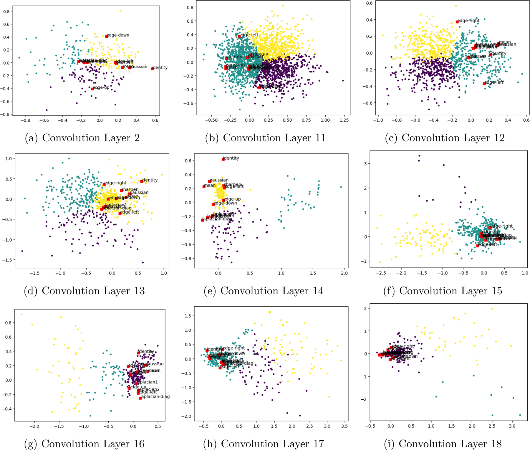
Visualization of 3×3 convolution kernels from selected layers of a UNet with a depth of 4. Colors correspond to K-means cluster assignment. Layers 1,3–10 (not shown) are similar to Convolution Layer 11. Layers 1–9 belong to the encoder portion of the UNet; layers 10–18 belong to the decoder. Observe that the further along the net, the more clustered the kernels become.

4. DISCUSSION

We demonstrate a flexible framework for using numerical analysis to provide insight into CNNs: we interpret upwind finite difference schemes as a convolution layers with ReLU activation functions. However, this alone is not sufficient to explain why CNNs are as accurate as they are. Our comparison between LSN, UNet and the level set equation illustrates that there are substantial differences in performance between each of these methods, despite the similarities in the mathematical mechanisms underlying the computational methods for each; UNet is the most successful of these methods, while LSN and the level set equation produce less accurate segmentations on the MICCAI LiTS dataset. Our subsequent kernel analysis visualizes the differences between kernels learned by the UNet and those used by the level set equation - the known kernels we superimpose on our clustering plots - where trends in clusters of the learned kernels begin to establish patterns in the decoder portions of our UNet. These patterns escape away from where the known level set equation kernels (and other common image processing kernels) are located on the clustering plots. Therefore, developing an understanding of the bottom layer and decoder portions of a CNN is a crucial step to being able to explain the predictive power of CNNs for image segmentation, which would enable an interpretation of convolution kernels in clinical terms.

REFERENCES

- 1.Ferlay J, Ervik M, Lam F, Colombet M, Mery L, Piñeros M, Znaor A, Soerjomataram I, and Bray F, “Global cancer observatory: Cancer today,” tech. rep., International Agency for Research on Cancer (2018). [Google Scholar]
- 2.McGlynn KA and London WT, “Epidemiology and natural history of hepatocellular carcinoma,” Best practice & research Clinical gastroenterology 19(1), 3–23 (2005). [DOI] [PubMed] [Google Scholar]
- 3.Bruix J, Reig M, and Sherman M, “Evidence-based diagnosis, staging, and treatment of patients with hepatocellular carcinoma,” Gastroenterology 150(4), 835–853 (2016). [DOI] [PubMed] [Google Scholar]
- 4.Heimbach JK, Kulik LM, Finn RS, Sirlin CB, Abecassis MM, Roberts LR, Zhu AX, Murad MH, and Marrero JA, “Aasld guidelines for the treatment of hepatocellular carcinoma,” Hepatology 67(1), 358–380 (2018). [DOI] [PubMed] [Google Scholar]
- 5.Bilic P, Christ PF, Vorontsov E, Chlebus G, Chen H, Dou Q, Fu C-W, Han X, Heng P-A, Hesser J, et al. , “The liver tumor segmentation benchmark (lits),” arXiv preprint arXiv:1901. 04056 (2019). [Google Scholar]
- 6.Heimann T, Van Ginneken B, Styner MA, Arzhaeva Y, Aurich V, Bauer C, Beck A, Becker C, Beichel R, Bekes G, et al. , “Comparison and evaluation of methods for liver segmentation from ct datasets,” IEEE transactions on medical imaging 28(8), 1251–1265 (2009). [DOI] [PubMed] [Google Scholar]
- 7.Kainmüller D, Lange T, and Lamecker H, “Shape constrained automatic segmentation of the liver based on a heuristic intensity model,” in [Proc. MICCAI Workshop 3D Segmentation in the Clinic: A Grand Challenge], 109–116 (2007). [Google Scholar]
- 8.Wu W, Zhou Z, Wu S, and Zhang Y, “Automatic liver segmentation on volumetric ct images using supervoxel-based graph cuts,” Computational and mathematical methods in medicine 2016 (2016). [DOI] [PMC free article] [PubMed] [Google Scholar]
- 9.Hoogi A, Beaulieu CF, Cunha GM, Heba E, Sirlin CB, Napel S, and Rubin DL, “Adaptive local window for level set segmentation of ct and mri liver lesions,” Medical image analysis 37, 46–55 (2017). [DOI] [PMC free article] [PubMed] [Google Scholar]
- 10.Ronneberger O, Fischer P, and Brox T, “U-net: Convolutional networks for biomedical image segmentation,” in [International Conference on Medical image computing and computer-assisted intervention], 234–241, Springer; (2015). [Google Scholar]
- 11.He K, Zhang X, Ren S, and Sun J, “Deep residual learning for image recognition,” in [Proceedings of the IEEE conference on computer vision and pattern recognition], 770–778 (2016). [Google Scholar]
- 12.Chan TF and Shen JJ, [Image processing and analysis: variational, PDE, wavelet, and stochastic methods], vol. 94, Siam; (2005). [Google Scholar]
- 13.Caselles V, Kimmel R, and Sapiro G, “Geodesic active contours,” International journal of computer vision 22(1), 61–79 (1997). [Google Scholar]
- 14.Yushkevich PA, Piven J, Hazlett HC, Smith RG, Ho S, Gee JC, and Gerig G, “User-guided 3d active contour segmentation of anatomical structures: significantly improved efficiency and reliability,” Neuroimage 31(3), 1116–1128 (2006). [DOI] [PubMed] [Google Scholar]
- 15.Chan TF and Vese LA, “Active contours without edges,” IEEE Transactions on image processing 10(2), 266–277 (2001). [DOI] [PubMed] [Google Scholar]
- 16.Finlayson SG, Bowers JD, Ito J, Zittrain JL, Beam AL, and Kohane IS, “Adversarial attacks on medical machine learning,” Science 363(6433), 1287–1289 (2019). [DOI] [PMC free article] [PubMed] [Google Scholar]
- 17.Engstrom L, Tran B, Tsipras D, Schmidt L, and Madry A, “A rotation and a translation suffice: Fooling cnns with simple transformations,” arXiv preprint arXiv:1712.02779 (2017). [Google Scholar]
- 18.Ruthotto L and Haber E, “Deep neural networks motivated by partial differential equations,” arXiv preprint arXiv:1804. 04272 (2018). [Google Scholar]
- 19.Chen TQ, Rubanova Y, Bettencourt J, and Duvenaud DK, “Neural ordinary differential equations,” in [Advances in neural information processing systems], 6571–6583 (2018). [Google Scholar]
- 20.Chollet F et al. , “Keras: Deep learning library for theano and tensorflow,” URL: https://keras.io/k 7(8), T1 (2015). [Google Scholar]