decorate: differential epigenetic correlation test

Abstract

Motivation

Identifying correlated epigenetic features and finding differences in correlation between individuals with disease compared to controls can give novel insight into disease biology. This framework has been successful in analysis of gene expression data, but application to epigenetic data has been limited by the computational cost, lack of scalable software and lack of robust statistical tests.

Results

Decorate, differential epigenetic correlation test, identifies correlated epigenetic features and finds clusters of features that are differentially correlated between two or more subsets of the data. The software scales to genome-wide datasets of epigenetic assays on hundreds of individuals. We apply decorate to four large-scale datasets of DNA methylation, ATAC-seq and histone modification ChIP-seq.

Availability and implementation

decorate R package is available from https://github.com/GabrielHoffman/decorate.

Supplementary information

Supplementary data are available at Bioinformatics online.

1 Introduction

Large-scale functional genomics datasets measuring gene expression, histone modifications, chromatin accessibility and DNA methylation across tens to hundreds of individuals have given novel insights into disease biology (Bryois et al., 2018; De Jager et al., 2014; Fromer et al., 2016; Girdhar et al., 2018; Jaffe et al., 2016; Klein et al., 2019). In a typical study, researchers assay a set of individuals with a particular disease and compare the magnitude of each gene expression trait or epigenetic feature to the magnitude from a set of control individuals. Coexpression analysis of gene expression data can identify correlated genes and has become widely used in the transcriptomics field (Langfelder and Horvath, 2008). In addition, analysis of differential correlation of genes between disease and control individuals can give novel insight into disease biology (Zhang et al., 2013). Yet application of this analytical framework to study differential correlation of epigenetic assays, such as histone modifications, chromatin accessibility and DNA methylation, at a large-scale have been limited by the high computational cost, and the lack of scalable software and robust statistical tests.

Here, we present decorate, differential epigenetic correlation test, a computationally scalable R package to identify correlated epigenetic features that are proximal along a chromosome, perform differential correlation testing between subsets of the data, and visualize results.

2 Materials and methods

The goal of the analysis is to detect correlated local epigenetic features and test the null hypothesis that the correlation structure of a cluster, s, of epigenetic features, Y, is equivalent between set A (i.e. cases) and set B (i.e. controls):

$$H_0:\text{cor}(Y_s^{\mathrm{A}})=\text{cor}(Y_s^{\mathrm{B}}).$$ (1)

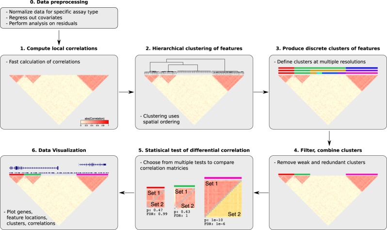
The challenge is to develop a workflow to evaluate the local correlation structure, identify clusters of epigenetic features at multiple resolutions, perform hypothesis tests on thousands of clusters and visualize the results on large-scale datasets. Decorate implements a computationally scalable seven-step workflow that can be applied to any genome-wide epigenetic assay after standard normalization and residualization for known confounders (Fig. 1).

Fig. 1.

Decorate workflow of seven steps including preprocessing, normalization and residualizing out confounders

2.1 Multivariate model and computing residuals

Consider a multivariate normal generative model

$$Y=\mathcal{N}\left(XB,\Sigma \right),$$ (2)

where $Y_{n\times p}$ is the matrix of epigenetic features with n samples and p features, $X_{n\times c}$ is a matrix of c covariates including the variable of interest, $B_{c\times p}$ is the matrix of p regression coefficients for c covariates and ${\Sigma }_{p\times p}$ is the matrix of covariances between all pairs of features. In addition, we consider the case where Σ only models local covariance structure so that ${\Sigma }_{i,j}=0$ when features i and j are greater than some pre-specified distance apart.

The expected covariance between two features ${{\displaystyle \overrightarrow{y}}}_i$ and ${{\displaystyle \overrightarrow{y}}}_j$ can be decomposed into (i) a global component modeling the covariates, and (ii) the local covariance structure:

$$E\left[\mathit{cov}\left({{\displaystyle \overrightarrow{y}}}_i,{{\displaystyle \overrightarrow{y}}}_j\right)\right]=\underset{\text{global}}{\underbrace{\mathit{cov}\left(X{{\displaystyle \overrightarrow{\beta }}}_i,X{{\displaystyle \overrightarrow{\beta }}}_j\right)}}+\underset{\text{local}}{\underbrace{{\Sigma }_{i,j}}}$$ (3)

where ${{\displaystyle \overrightarrow{\beta }}}_i$ and ${{\displaystyle \overrightarrow{\beta }}}_j$ are the vectors of regression coefficients for feature i and j, respectively. In practice, the local covariance structure can be estimated using the residuals of the each epigenetic feature after accounting for covariates:

$${\widehat{\Sigma }}_{i,j}=\mathit{cov}\left({{\displaystyle \overrightarrow{y}}}_i-X{\widehat{\beta }}_i,{{\displaystyle \overrightarrow{y}}}_j-X{\widehat{\beta }}_j\right).$$ (4)

The hypothesis tests are then performed on the corresponding correlation matrix because it is invariant to the scale of the features.

Since the focus of the analysis is on the local correlation structure and whether it differs between subsets of samples, it is essential to residualize out the global effects of covariates, including the variable of interest. Consider a dataset of two distinct cell types where thousands of epigenetic features have a different magnitude between the two cell types. In such a case, many features will then be correlated with cell type so that the global correlation structure will dominate the local correlation structure of interest. Analysis of the observed epigenetic features will not be able to identity much, if any, of local correlation structure or be able to test cell type-specific differences in correlation structure due to the strong global correlation structure (Supplementary Fig. S1). Based on first principles following from the generative model, biologically realistic simulations, and analysis of multiple datasets (see Section 3), we have found that the residualizing is a key part of the analysis workflow.

2.2 Compute correlations between local pairs of features

Computing the correlation between all pairs of features can be computationally prohibitive since it requires time and memory that increases quadratically with the number of features. In order to make this feasible on large datasets, decorate reduces the computational cost by evaluating only local correlations involving features within a fixed window. This can be achieved in linear time. Additional gains in speed are achieved by using extensive preprocessing to avoid redundant calculations, and by performing calculations efficiently using a C++ backend with RcppArmadillo (Eddelbuettel and Sanderson, 2014). Furthermore, decorate reduces memory usage from quadratic to linear by storing the results in a symmetric sparse matrix (Bates and Maechler, 2018). This is especially important for DNA methylation data with 450 K probes where storing all within-chromosome correlations requires 66 GB of memory, compared to just 4.8 GB using decorate with a window of 500 probes.

2.3 Perform hierarchical clustering of features

Stand ard hierarchical clustering is not adequate for epigenetic datasets since it is based on only the correlation matrix and ignores the spatial organization of features along the chromosome. Decorate applies two methods that explicitly model the spatial organization of epigenetic data. Adjacency constrained clustering (Ambroise et al., 2018; Dehman et al., 2015) is the stricter approach that only merges features that are adjacent on the chromosome as it constructs a hierarchical clustering. A more lenient approach, ClustGeo (Chavent et al., 2018), weighs both the correlation structure and the distance between each pair of features to encourage nearby features to be in the same cluster if the correlation structure supports it.

2.4 Produce discrete clusters of features

The hierarchical clustering must be split into discrete clusters for downstream analysis. Decorate applies a user-defined approach of setting the mean number of features in each cluster, or more sophisticated data-driven approaches. Clustering can be performed at multiple resolutions to produce hierarchically nested clusters.

2.5 Filter clusters based on strength of correlation

Initially, every epigenetic feature is assigned to a cluster. While some clusters contain features that are strongly correlated, other clusters do not have a strong correlation structure. In order to distinguish between these two cases, we report the lead eigenvalue fraction (LEF), the fraction of variance explained by the first eigenvalue. Large LEF values (i.e. >10%) indicate a strongly correlated set of features. Retaining only clusters that pass a cutoff value substantially reduces the multiple-testing burden. The value of the LEF cutoff can be determined empirically by shuffling the annotated genomic location of each feature in order to create a permuted dataset breaking the local correlations but retaining the global correlation structure.

In addition, discovering clusters at multiple resolutions can produce overlapping clusters. The overlapping clusters are identified and dropped from the analysis if the Jaccard index of the overlap passes a user-defined threshold.

2.6 Statistical test of differential correlation

The difference in correlation structure between subsets of the data can be evaluated for each discrete cluster using one of 15 statistical tests implemented in decorate. See Supplementary Material for details of methods and simulation study. Here, we focus on four methods favored by simulations for having high power while controlling the false-positive rate.

2.6.1 Sparse leading-eigenvalue-driven test

Sparse leading-eigenvalue-driven test (sLED) (Zhu et al., 2017) uses a form of sparse principal components analysis to test the leading eigenvalue of the difference between two correlation matrices compared to an empirical null distribution. Since the sLED statistic does not have a theoretical null distribution, the hypothesis test requires computationally expensive permutations. The stand ard implementation can be computationally intractable for large datasets and a multiple-testing burden of thousand s of tests. In order to scale this approach to large genome-wide datasets, decorate implements a parallelized, adaptive permutation approach that stops early for tests that are not close to significant. If a dataset contains 10 000 clusters, a P-value needs to be <0.05/10 000 = 5e−6 in order to be significant at a 5% Bonferroni cutoff. This requires at least 2e5 permutations, but likely an order of magnitude more to reduce Monte Carlo error. Analysis of a small simulated dataset with 500 samples on just 1000 features using 2e6 permutations on 20 CPU cores took only 4 min using decorate, but did not finish in 24 h with the original sLED implementation.

2.6.2 Box’s M test with permutations (Box.permute)

Box’s M statistic (Box, 1949) tests heterogeneity among multiple correlation matrices defined from discrete subsets of the data. The M statistic has a ${\chi }^2$ null distribution with the degrees of freedom determined by the number of samples and features. Yet this approach can give a high false-positive rate as the number of features increases. We used a fast permutation approach to draw 10 000 M statistics from the null distribution and then empirically estimate degrees of freedom of the ${\chi }^2$ null.

2.6.3 Correlation influence test of (delaneau)

Proposed by Delaneau et al. (2019), this test computes the correlation matrix $C=\mathit{cor}(Y_s)$ for a set of features s across all samples, and compares it to the correlation matrix, $C_{-i}$, computed when dropping sample i. The score for sample i, d_i, is the mean difference between C and $C_{-i}$ and indicates the influence of sample i on the correlation structure. Since this approach gives sample-level scores, it can be used to test association with both categorical and continuous variables. If this variable has two categories, a Wilcoxon test is used and for more than two categories a Kruskal–Wallis test is used. If the variable is continuous, a Spearman correlation test is used.

2.6.4 Sparse leading-eigenvalue-influence test (deltaSLE)

This test is similar to that of Delaneau et al. (2019), but tests the influence of each sample on the first eigenvalue. Letting λ be the sparse leading eigenvalue of correlation matrix C, and λ_i be the sparse leading eigenvalue of $C-C_{-i}$. The score for sample i, λ_i, indicates the influence of sample i on the correlation structure. A test of association with categorical or continuous variables is performed as above.

2.7 Data visualization

Gene annotations from any assembly (i.e. hg19 or hg38) are obtained from ensembldb (Rainer et al., 2019). Plotting is implemented using ggplot2 (Wickham, 2009).

2.8 Data analysis

DNA methylation, ATAC-seq and histone modification ChIP-seq data were analyzed with decorate using adjacency clustering using a window of 500 features, an LEF cutoff of 0.05, a Jaccard cutoff of 0.9, the Box.permute test and mean cluster size cutoffs ranging from 5 to 500 features to give clusters at multiple resolutions on each dataset. Spearman correlation was used to reduce the effect of outliers on the correlation structure. The effect of confounding variables from the original publication as well as variable of interest was residualized out before analysis with decorate. Importantly, this ensured that decorate analysis is driven only by differences in correlation rather than differences in feature magnitude between the groups of interest. Gene set enrichments were evaluated using GREAT (McLean et al., 2010). Analysis code and results are available at https://github.com/GabrielHoffman/decorate.

3 Results

3.1 Evaluating statistical methods for testing differential correlation

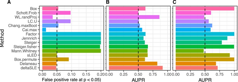
Simulations evaluating 15 statistical methods for testing differential correlation demonstrate substantial variability in ability to control the false-positive rate under the null (Fig. 2A). Moreover, there is substantial variability in the area under the precision-recall curve (AUPRC) across methods and simulation conditions (Fig. 2B and C).

Fig. 2.

Compare 15 statistical tests of differential correlation. Performance was evaluated for many combinations for sample size and number of features. The subset of simulation summarized here are for 100 samples and 15 features. (A) False-positive rate at p ¡ 0.05 under the null of no differential correlation. Dashed line indicates the target value of 0.05. (B) AUPRC under where all pairwise correlation in cases is 0.8 and in controls is 0.75. Dashed line indicates AUPRC of a rand om classifier. (C) AUPRC where all pairwise correlations are 0.80 in cases, and half of correlations in controls are set to 0.75 and the rest remain 0.80

3.2 Performance of decorate in simulations

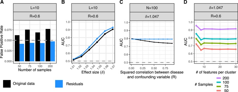
Biologically realistic datasets were simulated in order to evaluate the performance of the entire decorate workflow under a range of conditions. Simulations modeled locally correlated epigenetic features of L features per cluster, N case and N control samples, a differential correlation effect size δ and a confounding variable that has squared correlation with the disease status of R (see Supplementary Material). Under the null model of no differential correlation, analysis of the residuals after accounting for the confounding variable accurately controls the false-positive rate while analysis of the original data does not (Fig. 3A, Supplementary Fig. S2). Moreover, accounting for the confounding variable gives a higher area under the receiver operating characteristic curve (AUC) than analysis of the original data (Fig. 3B, Supplementary Fig. S3). The advantage of accounting for the confounding variable increases with the squared correlation between the disease and confounding variables (Fig. 3C, Supplementary Fig. S4). Finally, performance increases with sample size, but is not very sensitive to the number of features per cluster (Fig. 3D, Supplementary Fig. S5).

Fig. 3.

Evaluate false-positive rate and power from biologically realistic simulations. Simulate locally correlated epigenetic features of L features per cluster, N case and N control samples, a differential correlation effect size δ, and a confounding variable that has squared correlation with the disease status of R. Analysis was performed on either the original data (black) or the residuals after correcting for covariates (blue). The differential correlation test was performed with the Box.permute test on 3920 combinations of parameter values and a subset of summarized here. See Supplementary Material for details and additional simulation results. (A) False-positive rate under the null model of no differential correlation at P < 0.05 (gray dashed line) shown for analysis of the original data and residuals. (B) AUC over range of differential correlation effect sizes. Grey dashed line indicates AUC of a rand om classifier (C) AUC across a range of values for R. (D) AUC versus the number of features per clusters shown for multiple samples sizes. Note that 95% confidence intervals were computed for all AUC values, but they are too narrow to see here. (Color version of this figure is available at Bioinformatics online.)

3.3 DNA methylation from kidney renal clear cell carcinoma

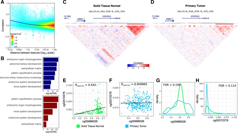
Analysis of DNA methylation from 160 primary tumor samples and 322 normal solid tissue samples assayed on the Illumina 450 K array and mapped to hg38 (Grossman et al., 2016) identified 99 152 clusters of correlated probes at multiple resolutions (Fig. 4). Pairs of probes within $\sim 1$ kb were enriched for being positively correlated compared to more distal probe pairs (Fig. 4A). Due to the massive genome-wide changes in DNA methylation associated with cancer, decorate identified 47 787 clusters comprising 279 540 probes that were differentially correlated between tumor and normal samples at FDR <5%. The genome-wide set of probes in differentially correlated clusters is enriched for kidney development compared to a background of all probes (Fig. 4B). For example, probes near PFKB3, a gene involved in glucose metabolism in cancer cells (Shi et al., 2017), are differentially correlated at FDR = 2.33e−72 (Fig. 4C and D). Visualizing a pair of probes from this cluster shows a large difference in Spearman correlation between normal (R = 0.442) and tumor (R = 0.000965) (Fig. 4E and F) despite the fact that there is no significant difference in magnitude between tumor and normal for these probes (Fig. 4G and H).

Fig. 4.

Analysis of DNA methylation from kidney renal clear cell carcinoma. (A) Pairwise correlation between probes on chr22 versus the distance between them. Color indicates density. Blue line shows non-parametric smooth. (B) Gene set enrichments for clusters with loss (blue) or gain (red) of correlation structure. (C) Correlation structure in normal solid tissue samples. (D) Correlation structure in primary tumor samples. (E) Correlation between two probes in normal tissue. (F) Correlation between same two probes in tumor. (G, H) Compare magnitude of same two probes between normal and tumor samples. (Color version of this figure is available at Bioinformatics online.)

3.4 DNA methylation from schizophrenia brain homogenate

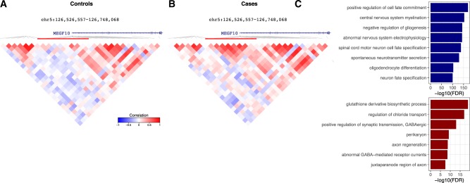
Analysis of DNA methylation from postmortem human brain homogenate from 108 individuals with schizophrenia and 136 controls on the Illumina 450 K array and mapped to hg19 (Jaffe et al., 2016) identified 61 823 clusters of correlated probes (Fig. 5). Decorate identified 49 clusters comprising 554 probes that were differentially correlated between schizophrenia and control samples. For example, probes near MEGF10, a gene involved in phagocytosis of apoptotic neurons in the brain (Iram et al., 2016), are differentially correlated at FDR = 0.031 (Fig. 5A and B). The genome-wide set of probes in differentially correlated clusters is enriched for neuronal and brain function compared to a background of all probes (Fig. 5C).

Fig. 5.

Analysis of DNA methylation from schizophrenia brain homogenate. (A) Correlation structure in control individuals. (B) Correlation structure in schizophrenia individuals. (C) Gene set enrichments for clusters with loss (blue) or gain (red) of correlation structure

3.5 ATAC-seq from schizophrenia brain homogenate

Analysis of ATAC-seq data from postmortem brain homogenate of 127 controls and 126 individuals with schizophrenia (Bryois et al., 2018; Hoffman et al., 2019) reprocessed to hg38 identified 24 572 clusters of correlated features. Decorate identified 7 clusters comprising 38 features that were differentially correlated between schizophrenia and control samples at FDR 10%.

3.6 Histone modification ChiP-seq from FACS-sorted human brain

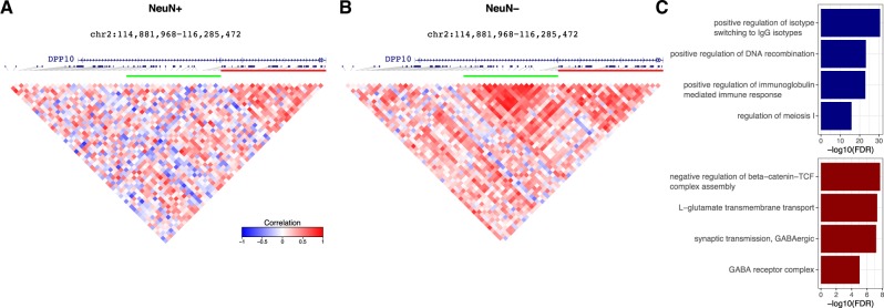
Analysis of histone modification ChIP-seq for H3K4me3 and H3K27ac from human postmortem brain of 17 individuals sorted based on NeuN to give neuronal and non-neuronal cells mapped to hg19 (Girdhar et al., 2018) identified 17 720 clusters of correlated ChIP-seq peaks (Fig. 6). Decorate identified 55 clusters comprising 516 peaks that were differentially correlated between neuronal and non-neuronal cell fractions. For example, peaks near DPP10, a gene associated with voltage-gated potassium channels (Bezerra et al., 2015), are differentially correlated at FDR = 3.2e−4 (Fig. 6A and B). The genome-wide set of peaks in differentially correlated clusters is enriched for neuronal function and cell replication compared to a background of all peaks (Fig. 6C).

Fig. 6.

Analysis of histone modification ChiP-seq from FACS sorted human brain. (A) Correlation structure in NeuN+ (i.e. neuronal) samples. (B) Correlation structure in NeuN− (i.e. non-neuronal) samples. (C) Gene set enrichments for clusters with loss (blue) or gain (red) of correlation structure

4 Conclusion

The decorate package enables statistical testing for differential epigenetic correlation in large-scale DNA methylation, ATAC-seq, histone modification ChIP-seq datasets. Decorate tests differences in the local correlation structure of multiple epigenetic features compared to a variable of interest, it is able to produce novel findings not identified by stand ard differential analysis comparing the magnitude of a single epigenetic feature. The genomic regions showing differential correlation in the datasets analyzed here give insight into the biology of the variable being tested (i.e. disease versus control, or neuronal versus non-neuronal cells). Notably, the number of differentially correlated features varies widely across datasets depending on the variable of interest, the sample size and the number of epigenetic features. Assays with a larger number of features, such as DNA methylation can detect more subtle correlation patterns and also increase power to identify differential correlation. Although, we focus here on comparisons of two subsets of the data, decorate implements tests that are directly applicable to multiple categories (i.e. Box.permute, delaneau and deltaSLE) as well as continuous variables (i.e. delaneau and deltaSLE).

The decorate workflow focuses on identifying differences in local correlation structure. We have illustrated through first principles following from the generative model, biologically realistic simulations and analysis of multiple datasets that accounting for relevant covariates is a key step in the workflow in order to accurately control the false-positive rate and maximize performance to identify differentially correlated clusters of epigenetic features.

Importantly, each analysis presented here took <2 h using 20 CPU cores. The computationally efficient implementation, simple R interface and publication quality visualizations will allow users to apply this analytical framework to a range of epigenetic datasets.

Funding

This work was supported by the National Institute of Mental Health [grants U01MH116442, R01MH109677, R01MH109897, R01MH110921]; the National Investigation Agency [grant R01AG050986]; and Veterans Affairs merit grant [BX002395 to P.R.]. It is partially supported by a NARSAD Young Investigator Award [26313 to G.E.H.] from the Brain and Behavior Research Foundation. This work was supported in part through the computational resources and staff expertize provided by Scientific Computing at the Icahn School of Medicine at Mount Sinai.

Conflict of Interest: none declared.

References

- Ambroise C. et al. (2018) adjclust: Adjacency-Constrained Clustering of a Block-Diagonal Similarity Matrix R package version 0.5.7 https://cran.r-project.org/package=adjclust (1 September 2019, date last accessed).
- Bates D., Maechler M. (2018) Matrix: Sparse and Dense Matrix Classes and Methods R package version 1.2-15.https://cran.r-project.org/package=Matrix (1 September 2019, date last accessed).
- Bezerra G.A. et al. (2015) Structure of human dipeptidyl peptidase 10 (DPPY): a modulator of neuronal Kv4 channels. Sci. Rep., 5, 8769. [DOI] [PMC free article] [PubMed] [Google Scholar]
- Box G.E.P. (1949) A general distribution theory for a class of likelihood criteria. Biometrika, 36, 317–346. [PubMed] [Google Scholar]
- Bryois J. et al. (2018) Evaluation of chromatin accessibility in prefrontal cortex of individuals with schizophrenia. Nat. Commun., 9, 3121. [DOI] [PMC free article] [PubMed] [Google Scholar]
- Chavent M. et al. (2018) ClustGeo: an R package for hierarchical clustering with spatial constraints. Comput. Stat., 33, 1799–1822. [Google Scholar]
- De Jager P.L. et al. (2014) Alzheimer’s disease: early alterations in brain DNA methylation at ANK1, BIN1, RHBDF2 and other loci. Nat. Neurosci., 17, 1156–1163. [DOI] [PMC free article] [PubMed] [Google Scholar]
- Dehman A. et al. (2015) Performance of a blockwise approach in variable selection using linkage disequilibrium information. BMC Bioinformatics, 16, 148. [DOI] [PMC free article] [PubMed] [Google Scholar]
- Delaneau O. et al. (2019) Chromatin three-dimensional interactions mediate genetic effects on gene expression. Science, 364, eaat8266. [DOI] [PubMed] [Google Scholar]
- Eddelbuettel D., Sand erson C. (2014) RcppArmadillo: accelerating R with high-performance C++ linear algebra. Comput. Stat. Data Anal., 71, 1054–1063. [Google Scholar]
- Fromer M. et al. (2016) Gene expression elucidates functional impact of polygenic risk for schizophrenia. Nat. Neurosci., 19, 1442–1453. [DOI] [PMC free article] [PubMed] [Google Scholar]
- Girdhar K. et al. (2018) Cell-specific histone modification maps in the human frontal lobe link schizophrenia risk to the neuronal epigenome. Nat. Neurosci., 21, 1126–1136. [DOI] [PMC free article] [PubMed] [Google Scholar]
- Grossman R.L. et al. (2016) Toward a shared vision for cancer genomic data. N. Engl. J. Med., 375, 1109–1112. [DOI] [PMC free article] [PubMed] [Google Scholar]
- Hoffman G.E. et al. (2019) CommonMind Consortium provides transcriptomic and epigenomic data for Schizophrenia and Bipolar Disorder. Sci. Data, 6, 180. [DOI] [PMC free article] [PubMed] [Google Scholar]
- Iram T. et al. (2016) Megf10 is a receptor for C1Q that mediates clearance of apoptotic cells by astrocytes. J. Neurosci., 36, 5185–5192. [DOI] [PMC free article] [PubMed] [Google Scholar]
- Jaffe A.E. et al. (2016) Mapping DNA methylation across development, genotype and schizophrenia in the human frontal cortex. Nat. Neurosci., 19, 40–47. [DOI] [PMC free article] [PubMed] [Google Scholar]
- Klein H.-U. et al. (2019) Epigenome-wide study uncovers large-scale changes in histone acetylation driven by tau pathology in aging and Alzheimer’s human brains. Nat. Neurosci., 22, 37–46. [DOI] [PMC free article] [PubMed] [Google Scholar]
- Langfelder P., Horvath S. (2008) WGCNA: an R package for weighted correlation network analysis. BMC Bioinformatics, 9, 559. [DOI] [PMC free article] [PubMed] [Google Scholar]
- McLean C.Y. et al. (2010) GREAT improves functional interpretation of cis-regulatory regions. Nat. Biotechnol., 28, 495–501. [DOI] [PMC free article] [PubMed] [Google Scholar]
- Rainer J. et al. (2019) ensembldb: an R package to create and use Ensembl-based annotation resources. Bioinformatics, 35, 3151–3153. [DOI] [PMC free article] [PubMed] [Google Scholar]
- Shi L. et al. (2017) Roles of PFKFB3 in cancer. Signal Transduct. Target. Ther., 2, 17044. [DOI] [PMC free article] [PubMed] [Google Scholar]
- Wickham H. (2009) ggplot2. Springer, New York, NY. [Google Scholar]
- Zhang B. et al. (2013) Integrated systems approach identifies genetic nodes and networks in late-onset Alzheimer’s disease. Cell, 153, 707–720. [DOI] [PMC free article] [PubMed] [Google Scholar]
- Zhu L. et al. (2017) Testing high-dimensional covariance matrices, with application to detecting schizophrenia risk genes. Ann. Appl. Stat., 11, 1810–1831. [DOI] [PMC free article] [PubMed] [Google Scholar]
Associated Data
This section collects any data citations, data availability statements, or supplementary materials included in this article.