

Abstract
Node centralities such as Degree and Betweenness help detecting influential nodes from local or global view. Existing global centrality measures suffer from the high computational complexity and unrealistic assumptions, limiting their applications on real-world applications. In this paper, we propose a new centrality measure, Node Conductance, to effectively detect spanning structural hole nodes and predict the formation of new edges. Node Conductance is the sum of the probability that node i is revisited at r-th step, where r is an integer between 1 and infinity. Moreover, with the help of node embedding techniques, Node Conductance is able to be approximately calculated on big networks effectively and efficiently. Thorough experiments present the differences between existing centralities and Node Conductance, its outstanding ability of detecting influential nodes on both static and dynamic network, and its superior efficiency compared with other global centralities.
Electronic supplementary material
The online version of this chapter (10.1007/978-3-030-47436-2_40) contains supplementary material, which is available to authorized users.
Keywords: Centrality, Network embedding, Influential nodes
Introduction
Social network analysis is used widely in social and behavioral sciences, as well as economics and marketing. Centrality is an old but essential concept in network analysis. Central nodes mined by centrality measures are more likely to help disseminating information, stopping epidemics and so on [19, 21].
Local and global centralities are classified according to the node influence being considered. Local centrality, for instance, Degree and Clustering Coefficient are simple yet effective metrics for ego-network influence. On the contrary, tasks such as information diffusion and influence maximization put more attention on the node’s spreading capability, which need centrality measurements at long range. Betweenness and Closeness capture structural characterization from a global view. As the measures are operated upon the entire network, they are informative and have been extensively used for the analysis of social-interaction networks [11]. However, exact computations of these centralities are infeasible for many large networks of interest today. The approximately calculated centralities also do not perform well in the real-world tasks [2, 6]. Moreover, these global centralities are sometimes unrealistic as their definitions are based on ideal routes, e.g., the shortest path. Yet, the process on the network usually evolves without any specific intention. Compared with the ideal routes, random walks are more realistic and easier to compute. This makes random-walk-based centrality outperforms other metrics in the real-world tasks [19].
We propose a new centrality, Node Conductance, measuring how likely is a node to be revisited in the random walk on the network. Node Conductance intuitively captures the connectivity of the graph from the target-node-centric view. Meanwhile, Node Conductance is more adequate in real applications by relaxing the assumption that information spreads only along ideal paths. Intuitively speaking, Node Conductance merges degree and betweenness centralities. Nodes with huge degree are more likely to be revisited in short random walks, and high betweenness nodes are more likely to be revisited in longer random walks. We further prove the approximability of Node Conductance from the induced subgraph formed by the target node and its neighborhoods. In other words, Node Conductance could be well approximated by the short random walks. This insight helps us calculate Node Conductance on big networks effectively and efficiently.
We then focus on the approximated Node Conductance, which is based on the revisited probability of short random walks on big networks. Specifically, we broaden the theoretical understanding of word2vec-based network embeddings and discover the relationships between the learned vectors, network topology, and the approximated Node Conductance.
In this paper, we positively merge two important areas, node centrality and network embedding. The proposed Node Conductance, taking the advantages of network embedding algorithms, is scalable and effective. Experiments prove that Node Conductance is quite different from the existing centralities. The approximately calculated Node Conductance is also a good indicator of node centrality. Compared with those widely used node centrality measures and their approximations, Node Conductance is more discriminative, scalable, and effective to find influential nodes on both big static and dynamic networks.
Related Work
Node Centrality. Centrality is a set of several measures aiming at capturing structural characteristics of nodes numerically. Degree centrality [1], Eigenvector Centrality [4], and Clustering coefficient [22] are widely used local centralities. Different from these centralities, betweenness [8] and Closeness [9] are somehow centrality measures from a global view of the network. The large computational cost of them limits the use on large-scale networks. Flow betweenness [5] is defined as the betweenness of node in a network in which a maximal amount of flow is continuously pumped between all node pairs. In practical terms, these three measures are sort of unrealistic as information will not spread through the ideal route (shortest path or maximum flow) at most times. Random walk centrality [19] counts the number of random walks instead of the ideal routes. Nevertheless, the computational complexity is still too high.
Subgraph centrality [7], the most similar measure to our work, is defined as the sum of closed walks of different lengths starting and ending at the vertex under consideration. It characterizes nodes according to their participation in subgraphs. As subgraph centrality is obtained mathematically from the spectra of the adjacency matrix, it also runs into the huge computational complexity.
Advance in NLP Research. Neural language model has spurred great attention for its effective and efficient performance on extracting the similarities between words. Skip-gram with negative sampling (SGNS) [16] is proved to be co-occurrence matrix factorization in fact [12]. Many works concerns the different usages and meanings of the two vectors in SGNS. The authors of [13] seek to combine the input and output vectors for better representations. Similarly, in the area of Information Retrieval, input and output embeddings are considered to carry different kinds of information [18]. Input vectors are more reflective of function (type), while output vectors are more reflective of topical similarity.
In our work, we further analyze the relationships between the learned input and output vectors and the network topology, bringing more insights to the network embedding techniques. Moreover, we bridge the gap between node embedding and the proposed centrality, Node Conductance.
Node Conductance (NC)
Conductance measures how hard it is to leave a set of nodes. We name the new metric Node Conductance as it measures how hard it is to leave a certain node. For an undirected graph G, and for simplicity, we assume that G is unweighted, although all of our results apply to weighted graphs equally. A random walk on G defines an associated Markov chain and we define the Node Conductance of a vertex i, NC , as the sum of the probability that i
is revisited at s-th step, where s
is the integer between 1 and
, as the sum of the probability that i
is revisited at s-th step, where s
is the integer between 1 and
 .
.
 |
1 |
The next section demonstrates that the number of times that two nodes co-occur in the random walk is determined by the sub-network shared by these two nodes. Node Conductance is about the co-occurrence of the target node itself and is thus able to measure how dense the connections are around the target node.
The Formalization of NC
The graph G is supposed to be connected and not have periodically-returned nodes (e.g. bipartite graph). The adjacency matrix  is symmetric and the entries equal 1 if there is an edge between two nodes and 0 otherwise. Vector
  , where
  is a
is a  vector of ones, n is the node number, and each entry of
  is the node degree.
  is the diagonal matrix of degree:
  . Graph G has an associated random walk in which the probability of leaving a node is split uniformly among the edges. For a walk starting at node i, the probability that we find it at j after exactly s steps is given by
 |
2 |
NC denotes the sum of the probability that the node is revisited at the step s, s is between 1 and r
 |
3 |
where  is the entry in the i-th row and i-th column of matrix
  .
.
Supposed that r approaches infinity, NC becomes a global node centrality measure. In order to compute the infinite sum of matrix power,
  is added for convenience.
 |
4 |
 , the Laplacian matrix
 of the network, is singular and cannot be inverted simply. We introduce pseudo-inverse.
  , where
  and
and  are the eigenvalue and eigenvector respectively. As vector [1, 1, ...] is always an eigenvector with eigenvalue zero, the eigenvalue of the pseudo-inverse
  is defined as follows.
  only concerns about the diagonal of
  .
.
 |
5 |
where  is the degree of node i, the ith entry of
  .
.
Although Node Conductance is a global node centrality measure, the Node Conductance value is more relevant with local topology. As shown in Eq. 3, in most cases, the entry value of  is quite small when s is large. It corresponds to the situation that the random walk is more and more impossible to revisit the start point as the walk length increases. In the supplementary material, we will prove that Node Conductance can be well approximated from local subgraphs. Moreover, as the formalized computation of Node Conductance is mainly based on matrix power and inverse, the fast calculation of Node Conductance is also required. We will discuss the method in Sect. 4.
Relationships to the Similar Centralities
Node Conductance seems to have very similar definition as Subgraph Centrality (SC) [7] and PageRank (PR) [20]. In particular, Node Conductance only computes the walks started and ended at the certain node. And PR is the stationary distribution of the random walk, which means that it is the probability that a random walk, with infinite steps, starts from any node and hits the node under consideration.  where the agent jumps to any other node with probability
  . The difference between
  and Eq. 4 lies in the random walks taken into account. By multiplying matrix
  , the PR value of node i is the sum of the entries in the i-th row of
  . In Eq. 4, the NC value of node i is the entry of the i-th row and i-th column. In summary, NC is more about the node neighborhood while PR is from a global view. The difference makes PageRank a good metric in Information Retrieval but less effective in social network analysis. After all, social behavior almost have nothing to do with the global influence.
SC counts the subgraphs number that the node takes part in, which is equivalent to the number of closed walks starting and ending at the target node,  The authors later add a scaling factor to the denominator in order to make the SC value converge, but get less interpretive. NC, on the contrary, is easy-to-follow and converges by definition.
Node Embeddings and Network Structure
As the calculation of Node Conductance involves matrix multiplication and inverse, it is hard to apply to large networks. Fortunately, the proof in our Supplementary Material indicates that Node Conductance can be approximated from the induced subgraph  formed by the k-neighborhood of node i. And the approximation error decreases at least exponentially with k. Random walk, which Node Conductance is based on, is also an effective sampling strategy to capture node neighborhood in the recent network embedding studies [10, 21]. Next, we aim at teasing out the relationship between node embeddings and network structures, and further introduces the approximation of Node Conductance.
Input and Output Vectors
word2vec is highly efficient to train and provides state-of-art results on various linguistic tasks [16]. It tries to maximize the dot product between the vectors of frequent word-context pairs and minimize it for random word-context pairs. Each word has two representations in the model, namely the input vector (word vector  ) and output vector (context vector
  ). DeepWalk [21] is the first one pointing out the connection between texts and graphs and using word2vec technique into network embedding.
Although DeepWalk and word2vec always treat the input vector  as the final result, context vector
  still plays an important role [18], especially in networks. (1) Syntagmatic: If word i and j always co-occur in the same region (or two nodes have a strong connection in the network), the value of
  is large. (2) Paradigmatic: If word i and j have quite similar contexts (or two nodes have similar neighbors), the value of
  is high. In NLP tasks, the latter relationship enables us to find words with similar meaning, and more importantly, similar Part-of-speech. That is the reason why only input embeddings are preserved in word2vec. However, we do not have such concerns about networks, and moreover, we tend to believe that both of these two relationships indicate the close proximity of two nodes. In the following, we analyze the detailed meanings of these two vectors based on the loss function of word2vec.
Loss Function of SGNS
SGNS is the technique behind word2vec and DeepWalk, guaranteeing the high performance of these two models. Our discussion of DeepWalk consequently starts from SGNS.
The loss function  of SGNS is as follows [12, 14].
  is the vocabulary set, i is the target word and
  is its context words set,
  is the number of times that j appears in the r-sized window with i being the target word.
  is the times that i appears in the training pairs:
  , where
  and
and  are the input and output vectors of i.
 |
6 |
 is the word sampled based on distribution
  , corresponding to the negative sampling parts, D is the collection of observed words and context pairs. Note that word2vec uses a smoothed distribution where all context counts are raised to the power of 0.75, making frequent words have a lower probability to be chosen. This trick resolves word frequency imbalance (non-negligible amount of frequent and rare words) while we found that node degree does not have such imbalanced distribution in all of the dataset we test (also reported in Fig. 2 in DeepWalk [21]). Thereby, we do not use the smoothed version in our experiments.
Dot Product of the Input and Output Vectors
SGNS aims to optimize the loss function  presented above. The authors of [12] provide the detailed derivation of SGNS as follows. We define
  and find the partial derivative of
  (Eq. 6 ) with respect to x:
  Comparing the derivative to zero, we derive that
  where k is the number of negative samples.
Node Conductance and Node Embeddings
In the above section, we derive the dot product of the input and output vectors. Now as for a certain node i, we calculate the dot product of its input vector and output vector:  Usually, the probability is estimated by the actual number of observations:
 |
7 |
P(i), namely the probability of a node being visited in a random walk, is proportional to the node degree. Thus, we have
 |
8 |
In our experiments, the value of  is used as the relative approximate Node Conductance value of node i. Actually, the exact value of each node’s Node Conductance is not that necessary. Retaining their relative ranks is enough to estimate their centrality.
The variants of DeepWalk also produce similar node embeddings. For example, node2vec is more sensitive to certain local structure [15] and its embeddings has lower capacity of generalization. We only discuss DeepWalk in this paper for its tight connection to random walk, which brings more interpretability than other embedding algorithms.
Implementation Details
DeepWalk generates m random walks started at each node and the walk length is l, sliding window size is w. Node embedding size is d. We set  ,
,  ,
,  , and
, and  . In order to compute the node embeddings, DeepWalk uses word2vec optimized by SGNS in gensim1 and preserves the default settings, where the embeddings are initialized randomly, initial learning rate is 0.025 and linearly drops to 0.0001, epochs number is 5, negative sample number is 5.
The formalized computation of Node Conductance is based on eigen-decomposition, which scales to  , V is the number of nodes. Using DeepWalk with SGNS, the computational complexity per training instance is
  , where n is the number of negative samples, w is the window size and d is the embedding dimension. The number of training instance is decided by the settings of random walks. Usually it is
  .
.
Comparison to Other Centralities
Now that different measures are designed so as to capture the centrality of the nodes in the network, it has been proved that strong correlations exist among these measures [23]. We compute different centrality measures on several small datasets2. NC is computed by Eq. 5. NC
 is computed by DeepWalk with the window size 6. As presented in Table 1, we calculate their correlations by Spearman’s rank correlation coefficient. NC
 and Network Flow Betweenness are not able to be computed on dataset polblog as the graph is disconnected. Apart from the football dataset, Degree, NC
 and PageRank value show significant relation with NC
 on all the rest datasets. Node Conductance is not sensitive to window size on these datasets.
Table 1.
Ranking correlation coefficient between the corresponding centralities and NC , Node Conductance with window size 6 (computed by Eq. 8). Centralities include Degree [1], NC
 (Eq. 5), Subgraph Centrality [7], Closeness Centrality [9], Network Flow Betweenness [5], Betweenness [8], Eigenvector Centrality [4], PageRank value [20], Clustering Coefficient [22].
| Metrics | Karate | Word | Football | Jazz | Celegans | Polblog | Pgp | |
|---|---|---|---|---|---|---|---|---|
| Degree |  |
 |
0.51 |  |
 |
 |
 |
 |
NC
|
 |
 |
0.41 |  |
 |
 |
– |  |
| Subgraph centrality | 0.71 |  |
0.48 | 0.85 | 0.66 |  |
 |
0.31 |
| Closeness centrality | 0.79 |  |
 |
0.84 | 0.45 |  |
 |
0.32 |
| Network flow betweenness |  |
 |
0.01 | 0.82 | 0.81 |  |
– |  |
| Betweenness | 0.84 |  |
 |
0.70 | 0.77 | 0.89 | 0.89 | 0.81 |
| Eigenvector centrality | 0.64 |  |
 |
0.85 | 0.66 | 0.87 |  |
0.30 |
| PageRank |  |
 |
0.48 |  |
0.83 |  |
 |
 |
| Clustering coefficient |  |
0.37 | 0.22 |  |
 |
0.33 | 0.20 | 0.59 |
We visualize the special case, football network, in order to have an intuitive sense of the properties of Degree, Betweenness, and Node Conductance (other centralities are presented in the Supplementary Material). Moreover, we want to shed more light on the reason why Node Conductance does not correlate with Degree on this dataset. Figure 1 presents the football network. The color represents the ranking of nodes produced by different metrics (Low value: red, medium value: light yellow, high value: blue). The values produced by these four metrics are normalized into range [0,1] respectively.
Fig. 1.

Network of American football games. The color represents the ranking of nodes produced by the metrics (Low value: red, medium value: light yellow, high value: blue). (Color figure online)
Comparing Fig. 1a and Fig. 1b with Fig. 1d, it seems that the result provided by Node Conductance (window = 6) synthesizes the evaluations from Degree and Betweenness. Node Conductance gives low value to nodes with low degree (node 36, 42, 59) and high betweenness centrality (node 58, 80, 82). We are able to have an intuitive understanding that Node Conductance captures both local and global structure characteristics.
When the window size is bigger, the distribution of node colors in Fig. 1c basically consistent with Fig. 1d. Some clusters of nodes get lower values in Fig. 1c because of the different levels of granularity being considered.
Application of Node Conductance
We employ Node Conductance computed by DeepWalk to both static network and dynamic network to demonstrate its validity and efficiency. Node Conductance of different window size are all tested and size 6 is proved to be the best choice. We try our best to calculate the baseline centralities accurately, while some of them do not scale to the big network datasets.
Static Network with Ground-Truth Communities (Table 2). We employ the collaboration network of DBLP, Amazon product co-purchasing network, and Youtube social network provided by SNAP3. In DBLP, two authors are connected only if they are co-authors and the publication venue is considered to be the ground-truth communities. DBLP has highly connected clusters and consequently has the best Clustering Coefficient (CC). In Amazon network, an edge means that two products are co-purchased frequently and the ground-truth communities are the groups of products that are in the same category. Users in Youtube social networks create or join into different groups on their own interests, which can be seen as the ground-truth. The link between two users represents their friend relationship. The CC of Youtube network is very poor.
Table 2.
The static network datasets.
| Datasets | Node | Edge |


|
CC 
|
|---|---|---|---|---|
| DBLP | 317K | 1M | 13K | 0.63 |
| Amazon | 335K | 926K | 75K | 0.40 |
| Youtube | 1.1M | 3.0M | 8K | 0.08 |
 Number of communities.
 Clustering Coefficient.
Dynamic Network. Flickr network [17] between November 2nd, 2006 and May 18th, 2007. As shown in Table 3, there are altogether 4 snapshots during this period. This unweighted and undirected network has about 300,000 new users and over 3.8 million new edges.
Table 3.
Snapshots of the Flickr network.
ss 
|
Node | Edge | ss | Node | Edge |
|---|---|---|---|---|---|
| 1 | 1,487,058 | 11,800,425 | 2 | 1,493,635 | 11,860,309 |
| 3 | 1,766,734 | 15,560,731 | 4 | 1,788,293 | 15,659,308 |
 ss stands for the number of snapshot.
Time Cost
The configuration of our computer is: two Intel(R) Xeon(R) CPU E5-2620 at 2.00 GHz, 64 GB of RAM. Node Conductance is calculated by DeepWalk with the setting  ,
,  ,
,  , and
, and  , the same setting in [21]. As Node Conductance is the by-product of DeepWalk, the actual running time of Node Conductance is the same as DeepWalk. As presented in the beginning of the section, Eigenvector centrality and PageRank are approximately calculated and we set the error tolerance used to check convergence in power method iteration to
  . Betweenness are approximately calculated by randomly choosing 1000 pivots. More pivots requires more running time. Subgraph Centrality and Network Flow Betweenness do not have corresponding approximations.
Time costs of some global centralities are listed in Table 4. Approximate Eigenvector, Subgraph Centrality and Network Flow Betweenness are not able to finish calculating in a reasonable amount of time on these three datasets. Node Conductance calculated by DeepWalk is as fast as the approximate PageRank and costs much less time than approximate Betweenness. Comparing with the existing global centralities, Node Conductance computed by DeepWalk is much more scalable and capable to be performed on big datasets.
Table 4.
Running time (seconds) of different global node centralities.
| Datasets | AP
|
NC
|
AB
|
AE
|
SC
|
FB
|
|---|---|---|---|---|---|---|
| DBLP | 914 | 985 | 14268 | – | – | – |
| Amazon | 941 | 988 | 9504 | – | – | – |
| Youtube | 2883 | 3464 | 168737 | – | – | – |
 approximate PageRank.
 Node Conductance.
 approximate Betweenness.
 approximate Eigenvector Centrality.
 Subgraph Centrality.
 Network Flow Betweenness.
Finding Nodes Spanning Several Communities
We use Node Conductance to find nodes spanning several communities. Sometimes, it is called structural hole as well. Amazon, DBLP and Youtube datasets provide the node affiliation and we count the number of communities each node belongs to. In our experiments, nodes are ranked decreasingly by their centrality values.
We first calculate the Spearman ranking coefficient between the ranks produced by each centrality measure and the number of communities. The error tolerance of approximate Eigenvector Centrality is set to be  . Other settings are the same as the Sect. 6.1. Results are shown in Table 5. Node Conductance performs the best and PageRank has a poor performance.
Table 5.
The Spearman ranking coefficient  of each centralities
 .
.
| Datasets |  |
 |
 |
 |
 |
 |
|---|---|---|---|---|---|---|
| DBLP | 0.62 | 0.60 | 0.61 | 0.59 | 0.48 | -0.29 |
| Amazon | 0.28 | 0.27 | 0.17 | 0.15 | 0.23 | 0.007 |
| Youtube | 0.26 | 0.24 | 0.23 | 0.21 | 0.20 | 0.22 |
 Subscript of
  stands for different centralities. D: Degree. Other subscripts are the same as defined in Table 4.
We further explore the differences between the rank of these centralities and plot the communities numbers of nodes (y-axis) in the order of each centrality measure (x-axis). In order to smooth the curve, we calculate the average number of communities node belongs to for every 1000 nodes. For example, point (x, y) denotes that nodes that are ranked from (1000x) to  belong to y communities on average. In Fig. 2, all of the six metrics are able to reflect the decreasing trend of spanning communities number. It is obvious that Node Conductance provides the smoothest curve comparing with the other five metrics, which indicates its outstanding ability to capture node status from a structural point of view. The consistency of performance on different datasets (please refer to the Supplementary Material) demonstrates that Node Conductance is an effective tool for graphs with different clustering coefficient.
Fig. 2.

Number of communities the node belongs to (Amazon dataset) versus node centrality calculated by different measures. The tails of the last two curves are marked as purple in order to emphasize the differences between the curves.
Degree and PageRank seem to have very different performances as shown in the Table 5, Fig. 2. The ground-truth centrality is the number of communities that each node belongs to, which means many nodes have the same centrality rank. Similarly, many nodes have the same degree too. However, under the measurement of the other centralities, nodes have different centrality values and ranks. Thus, degree has advantage to achieve higher ranking coefficient in Table 5 but performs bad as shown in Fig. 2. As for the curves of PageRank, the tails are quite different from the curves of Node Conductance. In Fig. 2e, the tail does not smooth. In other words, PageRank does not perform well for those less active nodes and thus achieves a poor score in Table 5.
The calculation of Node Conductance is entirely based on the topology, while node affiliation (communities) is completely determined by the fields and applications. Node affiliation is somehow reflected in the network topology and Node Conductance has better ability to capture it.
The Mechanism of Link Formation
In this experiment, we focus on the mechanism of network growing. It is well-known that the network growth can be described by preferential attachment process [3]. The probability of a node to get connected to a new node is proportional to its degree.
We consider the Flickr network [17] expansion during Dec. 3rd, 2006 to Feb. 3rd, 2007. Note that the results are similar if we observe other snapshots, and given space limitations, we only show this expansion in the paper. Nodes in the first snapshot are ranked decreasingly by their degree. We also count the newly created connections for every node. Figure 3 presents strong evidence of preferential attachment. However, there exist some peaks in the long tail of the curve and the peak should not be ignored as it almost reaches 50 and shows up repeatedly. Figure 3b presents the relationship between increasing degree and Node Conductance. Comparing the left parts of these two curves, Node Conductance fails to capture the node with the biggest degree change. On the other hand, Node Conductance curve is smoother and no peak shows up in the long tail of the curve. Degree-based preferential attachment applies to the high degree nodes, while for the nodes with fewer edges, this experiment suggests that there is a new expression of preferential attachment—the probability of a node to get connected to a new node is proportional to its Node Conductance.
Fig. 3.
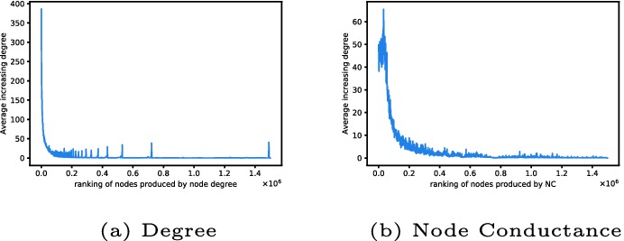
Preferential attachment.
Conclusion
In this paper, we propose a new node centrality, Node Conductance, measuring the node influence from a global view. The intuition behind Node Conductance is the probability of revisiting the target node in a random walk. We also rethink the widely used network representation model, DeepWalk, and calculate Node Conductance approximately by the dot product of the input and output vectors. Experiments present the differences between Node Conductance and other existing centralities. Node Conductance also show its effectiveness on mining influential node on both static and dynamic network.
Electronic supplementary material
Below is the link to the electronic supplementary material.
Acknowledgments
This work is supported by National Key Research and Development Program of China under Grant No. 2018AAA0101902, NSFC under Grant No. 61532001, and MOE-ChinaMobile Program under Grant No. MCM20170503.
Footnotes
Contributor Information
Hady W. Lauw, Email: hadywlauw@smu.edu.sg
Raymond Chi-Wing Wong, Email: raywong@cse.ust.hk.
Alexandros Ntoulas, Email: antoulas@di.uoa.gr.
Ee-Peng Lim, Email: eplim@smu.edu.sg.
See-Kiong Ng, Email: seekiong@nus.edu.sg.
Sinno Jialin Pan, Email: sinnopan@ntu.edu.sg.
Tianshu Lyu, Email: lyutianshu@pku.edu.cn.
Fei Sun, Email: ofey.sf@alibaba-inc.com.
Yan Zhang, Email: zhy@cis.pku.edu.cn.
References
- 1.Albert R, Jeong H, Barabasi AL. Internet: diameter of the world-wide web. Nature. 1999;401(6749):130–131. doi: 10.1038/43601. [DOI] [Google Scholar]
- 2.Bader DA, Kintali S, Madduri K, Mihail M. Approximating betweenness centrality. In: Bonato A, Chung FRK, editors. Algorithms and Models for the Web-Graph; Heidelberg: Springer; 2007. pp. 124–137. [Google Scholar]
- 3.Barabási AL, Albert R. Emergence of scaling in random networks. Science. 1999;286(5439):509–512. doi: 10.1126/science.286.5439.509. [DOI] [PubMed] [Google Scholar]
- 4.Bonacich P. Factoring and weighting approaches to status scores and clique identification. J. Math. Soc. 1972;2(1):113–120. doi: 10.1080/0022250X.1972.9989806. [DOI] [Google Scholar]
- 5.Borgatti SP. Centrality and network flow. Soc. Netw. 2005;27(1):55–71. doi: 10.1016/j.socnet.2004.11.008. [DOI] [Google Scholar]
- 6.Brandes U, Pich C. Centrality estimation in large networks. Int. J. Bifurcat. Chaos. 2007;17(07):2303–2318. doi: 10.1142/S0218127407018403. [DOI] [Google Scholar]
- 7.Estrada E, Rodrigue-Velaquez JA. Subgraph centrality in complex networks. Phys. Rev. E. 2005;71(5):056103. doi: 10.1103/PhysRevE.71.056103. [DOI] [PubMed] [Google Scholar]
- 8.Freeman LC. A set of measures of centrality based on betweenness. Sociometry. 1977;40(1):35–41. doi: 10.2307/3033543. [DOI] [Google Scholar]
- 9.Freeman LC. Centrality in social networks conceptual clarification. Soc. Netw. 1978;1(3):215–239. doi: 10.1016/0378-8733(78)90021-7. [DOI] [Google Scholar]
- 10.Grover, A., Leskovec, J.: node2vec: scalable feature learning for networks. In: Proceedings of KDD, pp. 855–864 (2016) [DOI] [PMC free article] [PubMed]
- 11.Kitsak M, Gallos LK, Havlin S, Liljeros F, Muchnik L, Stanley HE, Makse HA. Identification of influential spreaders in complex networks. Nat. Phys. 2010;6(11):888. doi: 10.1038/nphys1746. [DOI] [Google Scholar]
- 12.Levy, O., Goldberg, Y.: Neural word embedding as implicit matrix factorization. In: Proceedings of NIPS, pp. 2177–2185 (2014)
- 13.Levy, O., Goldberg, Y., Dagan, I.: Improving distributional similarity with lessons learned from word embeddings. In: Proceedings of ACL, pp. 211–225 (2015)
- 14.Li, Y., Xu, L., Tian, F., Jiang, L., Zhong, X., Chen, E.: Word embedding revisited: a new representation learning and explicit matrix factorization perspective. In: Proceedings of IJCAI, pp. 3650–3656 (2015)
- 15.Lyu, T., Zhang, Y., Zhang, Y.: Enhancing the network embedding quality with structural similarity. In: Proceedings of CIKM, pp. 147–156 (2017)
- 16.Mikolov, T., Sutskever, I., Chen, K., Corrado, G.S., Dean, J.: Distributed representations of words and phrases and their compositionality. In: Proceedings of NIPS, pp. 3111–3119 (2013)
- 17.Mislove, A., Koppula, H.S., Gummadi, K.P., Druschel, P., Bhattacharjee, B.: Growth of the flickr social network. In: Proceedings of WOSN, pp. 25–30 (2008)
- 18.Nalisnick, E., Mitra, B., Craswell, N., Caruana, R.: Improving document ranking with dual word embeddings. In: Proceedings of WWW, pp. 83–84 (2016)
- 19.Newman ME. A measure of betweenness centrality based on random walks. Soc. Netw. 2005;27(1):39–54. doi: 10.1016/j.socnet.2004.11.009. [DOI] [Google Scholar]
- 20.Page, L.: The pagerank citation ranking: bringing order to the web. Stanford Digital Libraries Working Paper (1998)
- 21.Perozzi, B., Al-Rfou, R., Skiena, S.: Deepwalk: online learning of social representations. In: Proceedings of KDD, pp. 701–710 (2014)
- 22.Watts DJ, Strogatz SH. Collective dynamics of a small-world networks. Nature. 1998;393(6684):440–442. doi: 10.1038/30918. [DOI] [PubMed] [Google Scholar]
- 23.Wuchty S, Stadler PF. Centers of complex networks. J. Theor. Biol. 2003;223(1):45–53. doi: 10.1016/S0022-5193(03)00071-7. [DOI] [PubMed] [Google Scholar]
Associated Data
This section collects any data citations, data availability statements, or supplementary materials included in this article.