Heterochromatin drives compartmentalization of inverted and conventional nuclei

Abstract

The mammalian cell nucleus displays a distinct spatial segregation of active euchromatic from inactive heterochromatic genomic regions^1,2. In conventional nuclei, microscopy shows that euchromatin is localized in the nuclear interior and heterochromatin at the nuclear periphery^1,2. Hi-C shows this segregation as a plaid pattern of enriched contacts between A (euchromatic) and B (heterochromatic) compartments³. Many mechanisms of compartment formation have been proposed, such as attraction of heterochromatin to the nuclear lamina^2,4, preferential attraction of similar chromatin to each other^1,4–12, higher levels of chromatin mobility in the active chromatin^13–15, and transcription-related clustering of euchromatin^16,17. Still, these hypotheses have remained inconclusive due to the difficulty of disentangling intra-chromatin and chromatin-lamina interactions in conventional nuclei¹⁸. The dramatic re-organization of interphase chromosomes in the inverted nuclei of rods in nocturnal mammals^19,20 provides an opportunity to elucidate mechanisms underlying spatial compartmentalization. Here we combine Hi-C analysis of inverted rod nuclei with microscopy and polymer simulations. We find that attractions between heterochromatic regions are crucial for establishing both compartmentalization and the concentric shells of pericentromeric heterochromatin, facultative heterochromatin, and euchromatin in the inverted nucleus. When interactions between heterochromatin and the lamina are added, the same model recreates the conventional nuclear organization. Models additionally allow us to rule out mechanisms of compartmentalization involving strong euchromatin interactions. Together, our experiments and modeling suggest that attractions between heterochromatic regions are central to phase separation of the active and inactive genome in inverted and conventional nuclei, while interactions with the lamina are essential for building the conventional architecture from these segregated phases.

To test mechanisms of genome compartmentalization, we performed Hi-C in four mouse cell types isolated from primary tissues that have either conventional or inverted nuclear architectures: rod photoreceptors (inverted), non-rod retinal neurons (conventional), wild type (WT) thymocytes (conventional), and lamin B receptor-null (LBR-null) thymocytes^20,21 (inverted) (Fig. 1a,), each with two biological replicates (ED Fig. 1; Table S1). The latter three cell types provide excellent points of comparison to rods: retinal non-rod neurons are similarly post-mitotic but have large conventional nuclei; WT and LBR-null thymocytes are cycling cells with nuclei of a size similar to rods. Nuclear inversion of LBR-null thymocytes is incomplete, most likely due to regular cell divisions (ED Fig. 2). Despite the great differences in nuclear organization evident from microscopy (Fig. 1a), all features of chromatin organization characteristic of conventional nuclei – Topologically Associating Domains (TADs), chromosome territories, and compartments – are present in inverted nuclei, although with quantitative differences (Fig. 1b; ED Fig. 3,4,5).

Figure 1. Microscopy and Hi-C analysis of conventional and inverted nuclei.

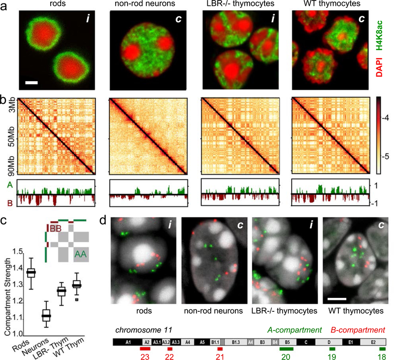
a, Nuclei of non-rod neurons and WT thymocytes are conventional (c) with euchromatin residing in the interior. Rod nuclei are inverted (i) with а single central heterochromatic region (including chromocenter) and euchromatin forming the peripheral shell. Nuclei of LBR-null thymocytes are partially inverted and have several chromocenters. Euchromatin staining with anti-H4K8ac antibody (green); counterstain with DAPI (red), highlighting heterochromatin; single optical sections; scale bar, 2 μm. See ED Fig. 9a3 and 10a for schematic of positioning of euchromatin, heterochromatin and chromocenters.

b, Hi-C contact maps (log10 contact frequency) for an 87 Mb region of chr1 (mm9) and corresponding compartment profiles indicating regions in the A (green) and B (dark-red) compartment (see also ED Fig. 1). Maps are corrected by ICE²², with the matrix sums normalized to one (Methods).

c, Compartmentalization is strongest in rods and weakest in non-rod neurons; schematic indicates how compartmentalization is quantified ((AA+BB)/total). Boxplots show compartmentalization calculated separately for each autosome in two replicas. Centerline shows the median, box shows lower and upper quartiles, whiskers extend to 1.5 times the interquartile range (see also ED Fig. 5).

d, Flipped localization of A and B compartment loci on chromosome 11 in inverted (i) compared to conventional (c) nuclei. Positions of detected compartments are marked with green (A-compartment) and red (B-compartment) bars below the chromosome ideogram. FISH with a BAC cocktail probe; BAC numbers are indicated below the compartment loci. Note the chromocenters seen as bright globules in DAPI staining. Projections of 3 μm confocal stacks; scale bar, 2 μm. The experiment was repeated twice.

We subsequently ask whether major differences in spatial positioning of euchromatin and heterochromatin affect nuclear compartmentalization as seen in Hi-C. We computed compartment profiles from Hi-C maps²² (Fig. 1b) and defined the degree of compartmentalization as the enrichment of contacts between compartments of the same type (Methods). While assignments of individual regions to A/B-compartments are generally cell-type dependent, compartment profiles before and after perturbing lamina association in thymocytes are highly correlated, approaching the correlation of biological replicates (ED Fig. 5b–e). The degree of compartmentalization decreases only slightly in thymocytes upon inversion but becomes stronger in rods (Fig. 1c; ED Fig. 5f). Taken together, our analyses show that the degree of compartmentalization is preserved despite the altered spatial positioning of individual A or B compartments upon inversion (Fig. 1a,d), and suggest that mechanisms of compartmentalization cannot be strictly dependent on the nuclear lamina.

To reconcile the remarkably similar Hi-C compartmentalization of inverted and conventional nuclei with their strikingly different spatial geometries, we sought a mechanism of compartmentalization that satisfied the three following criteria. First, it should reproduce the inverted organization, defined quantitatively with microscopy by the radial positions of different chromatin types and with H-C by the strength of compartmentalization. Second, it should reproduce the conventional organization when attractive interactions between heterochromatin and the nuclear lamina are introduced. The conventional organization is characterized by a similar degree of compartmentalization in Hi-C, but a drastically different spatial location of compartments in microscopy. Third, it should be based on biologically and physically plausible forces. This limited us to short-range attractions between different chromatin types and of chromatin to the nuclear lamina.

To test mechanisms of compartmentalization, we developed an equilibrium polymer model of chromatin that represents chromosomes as block copolymers (Fig. 2a), similar to other phase-separation models of compartmentalization^4–7. Extending previous two-type models, our simulations use 3 types of monomers: euchromatin (A), heterochromatin (B), or pericentromeric constitutive heterochromatin (C). We modeled 8 chromosomes, each consisting of 6000 monomers of ~40kb, confined to a spherical nucleus at 35% volume density²³. The sequence of A and B monomers along the polymer mirrors the sequence of compartments derived from Hi-C data of rods (Fig. 2a; Methods). To represent the satellite repeats of a pericentromeric region²⁴, or chromocenter, which is unmappable by Hi-C, we place a block of C monomers (16% of chromosome length) at the proximal end of each chromosome. All monomers have excluded volume, and experience short-range pairwise attraction depending on their chromatin type. Given six pairwise attraction parameters (A-A, A-B, B-B, B-C, C-C, A-C), all possible permutations of attraction strengths specify 720 (6!) classes of models (see Methods). To constrain the space of possible models, we first quantitatively compared all 720 classes of models to microscopy. Specifically, we computed the radial distributions for A, B, and C monomers, and compared these distributions between simulations and microscopy¹⁹ (Fig. 2b; Methods).

Figure 2. Morphology of the inverted nucleus restricts possible models of compartmentalization.

a, Our approach is to: (i) define mechanistic polymer models with parameters describing chromatin interactions between three types of monomers (A for euchromatin, B for heterochromatin, and C for constitutive heterochromatin), (ii) simulate an ensemble of conformations for each model via Langevin dynamics, and (iii) compare simulations with experiments. To compare to microscopy we compute radial distributions of A, B, and C monomers. Models are characterized by relative attraction strengths between every pair of monomer types, leading to 720 (6!) classes of models. For analysis, other models, see ED Fig. 6.

b. Quantitative comparison of 720 model classes with microscopy via the density peak distance, measuring the euclidean distance between the peaks of the radial distributions for each chromatin class in simulations and experiments (white dot). Simulated densities computed from 50 configurations, experimental data from 24 nuclei¹⁹.

c, Arranging the 720 models according to agreement with experimental data (i.e. density peak distance, Methods). Best 8 models (0–7) indicated in cyan. Other models plotted in black, or pink if representative conformation is shown from that model. Models 8–15 shown in ED Fig. 6a.

d, Heatmap (top, individual models) and barplot (bottom, averaged) of best 8 model parameters show they increase on average as AA ~ AB < AC < BB < BC < CC.

Most model classes do not agree with the concentric geometry of the inverted nucleus seen in microscopy (Fig. 2c). For example, overly strong B-C interactions cause B and C to mix (Fig. 2c, model 8; ED Fig. 6a–c), while relatively weak B-C interactions lead to the expulsion of the C monomer chromocenters from a central mass of B monomers (Fig.2c, model 112). Overly strong A-A interactions tend to encourage the formation of large euchromatic globules (Fig.2c, model 650; ED Fig.6d–f). Importantly, this result argues against activity-related clustering of euchromatic regions^13–16 as the main mechanism underlying compartmentalization.

Only eight classes of models could reproduce the experimentally observed inverted geometry (Fig. 2b,c). These eight classes follow a particular ordering of interaction strengths, on average dominated by heterochromatic interactions: A-A ≤ A-B ≤ A-C ≤ B-B < B-C < C-C (Fig. 2d). We focused on the best fitting class of models and further simplified it by fixing C-C to be high enough to induce a central globule of C monomers, A-A to always be much smaller than B-B (ED Fig. 7d), and all cross terms to be the geometric means of the respective pure terms (e.g. A-B = (A-A × B-B)^1/2), thereby satisfying the Flory-Huggins phase separation criterion²⁵. This leaves the B-B attraction as the only free parameter.

We next tested if the heterochromatin-dominated models that reproduced the inverted organization seen in microscopy could simultaneously reproduce the compartmentalization observed in Hi-C data. Fixing the order of interaction strengths, we found a range of the B-B attractive energy where models could quantitatively reproduce both Hi-C and microscopy (Fig. 3a,b). The central role of attractions between heterochromatic regions revealed by our analyses of inverted nuclei contrasts with suggestions hinging on the importance of interactions between euchromatic regions^13–16 or with the lamina² as the main drivers of compartmentalization. The strength of heterochromatic attractions is consistent with the dominant role of heterochromatin-associated methylation recently identified in the mechanics of mitotic chromosomes²⁶.

Figure 3. Heterochromatin-based mechanisms quantitatively reproduce inverted and conventional nuclei.

a-b, model for the inverted nucleus. Starting with the parameter ordering required to reproduce the morphology of the inverted nucleus (Fig. 2), we then varied B-B interactions to find models that best agree with Hi-C and microscopy data.

a, Compartment strength as a function of B-B attraction (boxes as in Fig. 1c, with 8 simulated chromosomes averaged across 150 conformations). Orange lane shows compartment strength from rod Hi-C (see Fig. 1c). Blue region shows parameter range in agreement with Hi-C. (i ,ii, iii) Simulated Hi-C maps (log10 contact frequency, chr1:50Mb-chr1:150Mb) are shown for indicated values of B-B. Model (ii) agrees best with Hi-C compartment strength. Attracting a small number of B monomers to the nuclear periphery does not disrupt the inverted architecture (ED Fig. 7a).

b, Distance between model and microscopy (as in Fig. 2b,c) as a function of B-B attraction (averaged over 150 conformations, boxes as in Fig. 1c). Purple lane shows agreement with microscopy (Methods) when B-B attraction strength is above 0.4kTAs above, blue region as in (a). Representative conformations shown to the right (i, ii, iii).

c-d, model for the conventional nucleus. The model for conventional nuclei additionally includes interactions of monomers with the nuclear lamina. B monomers are attracted to the lamina with a strength B-Lam and C monomer clusters are pinned to the lamina at random positions.

c, Compartment strength as function of B-B and B-Lam attractions (calculated as in Fig. 3a, over 8 simulated chromosomes). (iv-vii) Simulated Hi-C maps displayed for indicated parameters. Experimental compartment strength (orange outline, for conventional WT thymocytes) can be matched (point vi) even if B-B interactions are costrained to be the same as for inverted nuclei (blue outline, range from Fig. 3a).

d, Distance between microscopy and models (calculated as in Fig. 3b, over 150 simulated conformations). (iv-vii) conformations for indicated parameters. Agreement with microscopy (purple lines) and Hi-C (blue lines) is simultaneously achievable with B-B attraction strength from our inverted nucleus model (iv). Attracting a small number of A monomers to the periphery, or tethering a fraction of chromocenters to the interior does not alter our conclusions (ED Fig. 7).

To extend our model to conventional nuclei, we represented heterochromatin-lamina interactions with a short-ranged attraction^2,20 (B-Lam attraction, Fig. 3c,d). To model distinct chromocenters seen experimentally, we pinned C-monomer clusters to random positions along the lamina. Pinning is not necessary to maintain distinct chromocenters for a period of time, but is needed to keep them separated in equilibrium simulations (Supplementary Video 1). By sweeping B-B and B-Lam attractions, we found that our model can simultaneously reproduce both the spatial positioning of active and inactive chromatin as observed in microscopy. While reproducing microscopy requires sufficiently strong B-Lam without further constraining these parameters, simultaneously reproducing the compartmentalization observed in Hi-C data on WT thymocytes narrows down the range of B-Lam and B-B attraction (Fig. 3c,d). Interestingly, the region of best-fitting B-B attraction for conventional nuclei includes the best-fitting B-B attraction for inverted nuclei. Since histone modifications remain associated with the same type of chromatin in inverted and conventional nuclei^20,21, we parsimoniously assume that B-B attraction remains the same in both nuclear types. With this constraint, we can narrow the range of possible B-Lam values (~0.3 kT, Fig. 3c) and find that B-Lam attraction should be comparable to B-B attraction. Taken together, our simulations argue that compartmentalization in both inverted and conventional nuclei is primarily controlled by heterochromatin-heterochromatin attractions, while heterochromatin-lamina attraction controls the global spatial morphology.

To test our proposed mechanism of compartmentalization, we simulated a time-course of nuclear inversion (Fig. 4a–b). For this, we turned off lamina-heterochromatin interactions in simulated conventional nuclei and observed spontaneous inversion (Fig. 4b1). Remarkably, the simulated time-course mirrored key events during rod differentiation in vivo^19,20 (Fig. 4b2). B and C monomer droplets underwent irreversible liquid-like fusion in simulations, similar to in vitro phase-separated systems^10,11 (Fig. 4b; ED Fig. 8a,c; Supplementary Video 2). In simulations, although compartmentalization transiently dips after heterochromatin moves away from the lamina (Fig. 4a2), compartments remain separated during the whole process of inversion. In agreement with simulations, individual genomic loci reposition along with chromatin of their own compartment type during the entire process of rod nuclear inversion in vivo (ED Fig. 9). For example, the rhodopsin locus (Fig. 4c1) remains associated with euchromatin (A compartment), and the rhodopsin receptor remains expressed throughout the process of inversion (Fig. 4c2).

Figure 4. The time-course and maintenance of compartment strength during nuclear inversion in the model and experiment.

a, Simulated nuclear inversion. Configurations indicated by numerals and thin lines are displayed in (b). Solid vertical line indicates the time at which interactions with the lamina are eliminated. (a1) C monomers move towards the nuclear interior following removal of lamina interactions. Light lines are computed from individual simulations, dark lines show their average. (a2) Compartment strength is maintained during inversion, showing only a transient dip.

b, Representative conformations from simulations (b1; see also ED Fig. 8a) mirror changes in chromatin architecture during rod differentiation in vivo (b2) detected by FISH with probes for Long Interspersed Nuclear Elements (LINEs, L1, red), Short Interspersed Nuclear Elements (SINEs, B1, green) and major satellite (blue). The progression of geometries remains unchanged when simulated inversion is accompanied by volume decrease (ED Fig. 8c) in accordance with in vivo observations ¹⁹.

c1, In the process of nuclear inversion, the rhodopsin locus (red) within chromosome 6 (green) changes position from internal (empty arrowheads) to peripheral (solid arrowhead) but remains within the A compartment (see ED Fig. 9 for other genomic regions). c2, despite this dramatic relocation, Rhodopsin gene expression, which starts at P6, continues at an increasing rate. OS, outer segments of rods positive for rhodopsin staining (green); ONL, outer nuclear layer containing rod perikarya.

Single confocal sections (b2) and projections of 2 μm confocal stacks (c1, c2). Scale bars, 5 μm (b2, c1) and 50 μm (c2). P0-P21, and Ad indicate postnatal days and adult (3.5 months) in panels b1, c1, c2.

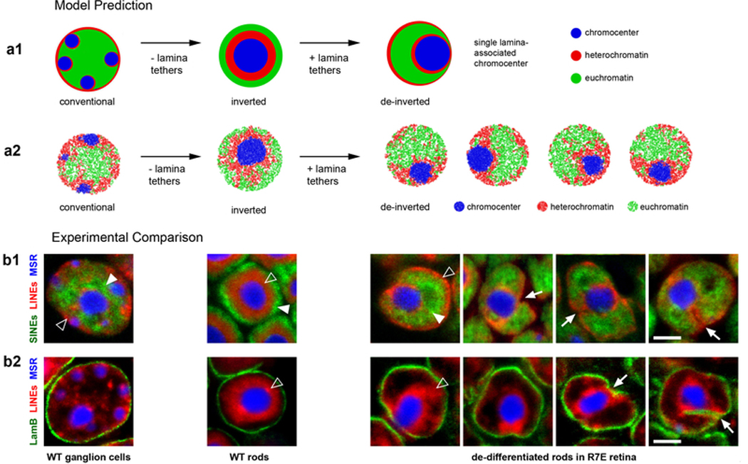
To further test our proposed mechanism of compartmentalization, we initialized simulations from an inverted geometry and re-introduced lamina-heterochromatin interactions. These simulations predicted only partial de-inversion: while B monomers replaced A monomers at the periphery of the nucleus, C monomers remained as a single large globule surrounded by B monomers and associated with the lamina (ED Fig. 10a). We tested these predictions experimentally by imaging de-differentiating rods of R7E mice that express polyQ-expanded ataxin-7²⁷. Rods in these mice start lamin A/C expression after their nuclear inversion is completed²⁰ and acquire partially de-inverted morphologies remarkably similar to simulations (ED Fig. 10b).

Together, our results show the central role of interactions between heterochromatin in establishing compartmentalization by phase separation. Using polymer simulations to reconcile microscopy and Hi-C data, we find that: (i) interactions between heterochromatic regions lead to phase separation of chromatin, and are essential for the compartmentalization of conventional and inverted nuclei; (ii) euchromatic interactions are dispensable for compartmentalization; and (iii) lamina-heterochromatin interactions are dispensable for segregation of eu- and heterochromatin, but central in establishing the conventional nuclear architecture. While we narrow the search for key molecular determinants of compartmentalization to heterochromatin-associated molecules, making predictions for perturbations to particular molecular determinants remains a limitation of our current study. Candidates for mediators of heterochromatin-heterochromatin interactions include affinity between homotypic repetitive elements^1,9,28 or modified histones, and heterochromatin-associated proteins (e.g. HP1)^10,11. Future work should consider the interplay between the mechanisms considered here and other chromosomal processes, such as non-equilibrium decondensation after mitosis²⁹ and loop extrusion⁸. Broadly, our results indicate that the inverted nucleus conceptually represents the default nuclear architecture imposed by the mechanism of compartmental interactions, and the conventional nucleus requires additional lamina-heterochromatin interactions. Since most eukaryotic nuclei have a conventional organization, our work raises the question about the functional relevance of heterochromatin positioning at the nuclear periphery.

Methods

Cryosections and immunostaining

Cryosections.

Retina was sampled from CD1 mice at P0, P3, P6, P13, P21, P28, and 3.5 months. Samples of retinas from R7E mice were kindly provided by D.Devys, IGBMC, University of Strasbourg. For detailed protocol of tissue fixation and cryosection preparation, see⁴². Briefly, tissues were fixed with 4% formaldehyde in PBS for 20–24 h, washed with PBS, incubated in sucrose with increasing concentrations (10%, 20% and 30%) and transferred into embedding molds (Peel-A-Way® Disposable Embedding Molds, Polysciences Inc., USA) filled with Jung freezing medium (Leica Microsystems). Tissue cryoblocks were frozen by immersing the molds into a −80°C ethanol-bath, and stored at −80°C. Cryosections with a thickness of 16–20 μm were cut using a Leica Cryostat (Leica Microsystems), collected on SuperFrost microscopic slides (SuperFrost Ultra Plus, Roth, Germany), immediately frozen and stored at −80°C before use.

Immunostaining.

Rhodopsin expression during rod differentiation was studied with antibodies to rhodopsin (RET-P1, Abcam). Nuclear architecture of retinal cells in degenerating retina of R7E mice was studied using antibodies for the euchromatin marker histone modification H3K9ac (kindly donated by H.Kimura, Tokyo Institute of Technology, Yokohama), ATAXN7 (kindly provided by D.Devys, IGBMC, University of Strasbourg) and lamin A/C (kindly provided by H.Herrmann, DKFZ, Heidelberg). Secondary antibodies were conjugated to Alexa 488, Alexa 555, Alexa 594 or Alexa 647 (Invitrogen). For detailed description of the immunostaining protocol, see⁴³. Briefly, sections were incubated with primary and secondary antibodies diluted in blocking solution (1% BSA + 0.1% TritonX100 + 0.1% saponin) under glass chambers for 18–20 h at RT. Washings (3 × 30 min) in-between and after antibody incubations were performed with 0.05% TritonX100/PBS at 37°C. For the nuclear counterstaining, DAPI was added to the secondary antibody solution to a final concentration of 2 mg/ml.

FISH and microscopy

FISH.

FISH on cryosections was performed according to the previously published protocol⁴². Briefly, cryosections were dried up for 30 min at RT, re-hydrated in 10 mM sodium citrate buffer (pH 6.0) and heated in the same buffer for 30 min at 80°C for antigen retrieval. After equilibration with 2xSSC buffer and incubation with 50% formamide/2xSSC for 30 min, probes were loaded on cryosections under small glass chambers, sealed with rubber cement and preincubated on a hot block at 45°C for 1 h. Tissue and probe DNA were denatured simultaneously on a hot block at 80°C for 3–5 min. Hybridization was carried out at 37°C for 2 days. After posthybridization washings with 2xSSC at 37°C and 0.1xSSC at 61°C, sections were counterstained with 2 μg/ml DAPI for 1h and mounted in Vectashield antifade medium (Vector Laboratories).

FISH probes.

BAC clones used in the study were purchased from BACPAC Resources (Childreńs hospital Oakland). For coordinates of all BACs see Supplementary Table S2. BAC DNA was amplified from a miniprep using GenomiPhi kit (GE Healthcare, UK), labeled by nick translation with fluorochrome-conjugated nucleotides and purified using QIAquick Nucleotide Removal Kit 50 (Qiagen). dUTPs were labeled with FITC, Cy3, TexasRed or Cy5 according to the published protocol⁴⁴. To verify BAC clones and exclude those that cross-hybridize to other chromosomes, all BAC probes were first labeled with Dig-dUTP and co-hybridized with a respective chromosome paint labeled with Bio-dUTP to mouse metaphase spreads. Hybrids were detected with anti-Dig antibody conjugated to FITC (Jackson Immuno Research) and avidin conjugated to Alexa555 (Invitrogen Molecular Probes). Mouse chromosome paints were a kind gift from Johannes Wienberg (University of Cambridge). The paints were first amplified and then labeled with Biotin-dUTP or Cy3-dUTP by DOP-PCR using 6MW primer (5´-CCG-ACTCGA-GNN-NNN-NAT-GTG-G-3´, Eurogentec). For FISH probe preparation, 4 μg of labeled BAC or 6 μg of a chromosome paint, were mixed with 10 μg of salmon sperm DNA and 50 μg of mouse Cot1 DNA, ethanol precipitated and dissolved in 10 μl of hybridization mixture consisting of 50% deionized formamide (Sigma–Aldrich), 10% dextran sulphate (Amersham Biosciences) and 1xSSC⁴². Probes for FISH with SINEs (B1) and LINEs (LINE1) and major satellite repeat are described in Solovei et al (2009)¹⁹.

Immuno-FISH.

For the nuclear lamina staining after FISH, sections were equilibrated in PBS and stained as described above using antibodies for lamin B1 (Santa Cruz, sc-6217), or lamin A/C and LBR (both kindly provided by H.Herrmann, DKFZ, Heidelberg).

Microscopy and image analysis.

Image stacks were acquired using Leica TCS SP5 confocal microscope equipped with Plan Apo 63×/1.4 NA oil immersion objective and lasers for blue (405 nm), green (488 nm), orange (561 nm), red (594 nm) and far-red (633 nm) fluorescence. Multichannel image stacks were corrected for chromatic shift and processed using a dedicated ImageJ plugin “Stack Groom”⁴⁵.

Animals

Mice used for tissue sampling were obtained from Charles River Laboratories, housed at the Biocenter, Ludwig Maximilians University of Munich (LMU) and treated according to the standard protocol approved by the Animal Ethics Committee of LMU.

Tissue sampling for Hi-C

Retinas from CD1 and C3H adult mice (retired breeders) were dissociated into single cell suspension using Papain Dissociation System (Worthington Biochemical Corporation) as described elsewhere⁴⁶. 4 retinas from 2 mice were used for one biological replica. To obtain a pure population of rod photoreceptors, retina suspensions were sorted based on standard forward and sideward scatter settings using FACS Aria II (Becton Dickinson) and yielded about 1 mln rod perikarya (Supplementary Fig. S1). Retinas of C3H mice, lacking the entire outer nuclear layer, were used to obtain the non-rod population of retinal neurons. Each biological replica of non-rod neurons contained ca. 10 mln cells. Thymocytes from WT CD1 mice and LBR-null mice⁴⁷ were extracted from thymuses of young adult animals, P26 and P28, respectively. Thymuses were minced, small tissue pieces were gently pipetted and the resulting single cell suspension was pressed through a Cell Strainer Snap Cap with a mesh size of 35 μm. Each biological replica of thymocytes contained 25–30 mln cells. Images of microscopic controls of isolated rods, non-rod neurons and thymocytes are shown in Supplementary Fig. S2. All cells were fixed with 1% formaldehyde (Fisher Scientific, cat # 10532955) for 10 min at RT. Fixation was quenched with 0.1M glycine for 5 min at RT and then for 15 min at 4ºC. Fixed cells were pelleted, snap-frozen and kept at −80ºC until use.

Hi-C

Hi-C was performed as described ⁴⁸ with modifications.

Cell lysis and chromatin digestion.

450 000 formaldehyde cross-linked rod nuclei and up to 5 mln of other cell types were incubated in 1ml of cold lysis buffer [1 ml 10 mM Tris-HCl pH8.0, 10 mM NaCl, 0.2% (v/v) Igepal CA630, mixed with 100 μl protease inhibitors (Sigma P8340) immediately before use] on ice for 15–20 minutes. Next, samples were lysed with a Dounce homogenizer and pestle A (KIMBLE Kontes # 885303–0002) by moving the pestle slowly up and down 25 times, incubating on ice for one minute followed by 10 more strokes with the pestle. The suspension was centrifuged for 5 minutes at 9,800 rpm (rod nuclei) and 4,500 rpm (all other samples) at RT using a table top centrifuge (Centrifuge 5810R, (Eppendorf). The supernatant from rod nuclei sample was carefully removed and spun second time (9,800 rpm 5min) and then both pellets were combined. Pellets were washed twice with ice cold 500 μl 1x NEBuffer 2 (NEB). After the second wash, each pellet was resuspended in 1x NEBuffer 2 in a total volume of 352 μl, chromatin was solubilized by addition of 38 μl 1% SDS per tube, the mixture was resuspended and incubated at 65°C for 10 minutes. Tubes were placed on ice and 44 μl of 10% Triton X-100 was added. Chromatin was subsequently digested by adding 400 Units HindIII (NEB) at 37°C for 15h with continuous slow rocking in parafilm-sealed tubes. Digested chromatin solution was spun shortly, transferred to ice and used for generating Hi-C libraries.

Biotin marking of DNA ends and blunt end ligation.

The HindIII DNA ends were filled in and marked with biotin by adding 70 μl fill-in mix [2 μl 10 mM dATP, 2 μl 10 mM dGTP, 2 μl 10 mM dTTP, 42 μl 0.4 mM biotin-14-dCTP (Invitrogen #19518–018), 7 μl 10x NEBuffer 2, and 15 μl 5U/μl Klenow polymerase (NEB M0210L)] followed by incubation at 37°C for 4 hours on rocking platform at 50 rpm. Klenow polymerase was inactivated by adding 96 μl 10% SDS followed by incubation at 65°C for 30 minutes. Tubes were then placed on ice immediately afterwards; the content of each of the tube was transferred to 15 ml conical tube containing 7.58 ml ligation mix [820 μl 10% Triton X-100, 758 μl 10x ligation buffer (500 mM Tris-HCl pH7.5, 100 mM MgCl2, 100 mM DTT), 82 μl 10 mg/ml BSA, 82 μl 100 mM ATP and 5.84 ml water]. 50 μl 1U/μl T4 DNA ligase (Invitrogen #15224) was added and mixed by inverting tubes; ligation was performed at 16°C overnight. For DNA purification, 50 μl of 10 mg/ml Proteinase K (Invitrogen # 25530–031) was added to each tube and samples were incubated at 65°C for 4 hours followed by a second addition of 50 μl of 10 mg/ml Proteinase K solution and 8 hours incubation at 65°C. Tubes were cooled to RT and DNA samples were transferred to 50 ml conical tubes. The DNA was extracted by adding an equal volume of phenol pH8.0 (Fisher BP1750I-400), vortexing for 3 minutes and spinning for 10 minutes at 4,000 rpm in a table top centrifuge (centrifuge 5810R, Eppendorf). The supernatants were transferred to new 50 ml conical tubes. Another two extractions were performed with an equal volume of phenol, pH8.0 : chloroform (1:1). Next, supernatants with HiC libraries were concentrated and desalted on 30 kDa Amicon Ultra-15 columns (Fisher UFC903024) by spinning for 10 minutes at 4,000 rpm in a table top centrifuge (centrifuge 5810R, Eppendorf) once. The flow through was discarded and each column was washed once with 5ml of mQ water. Then samples were dissolved in 1mL of 1 x TE buffer, transferred to 30 kDa Amicon Ultra 0.5 ml columns (Fisher UFC5030BK) and spun at 10 000rpm, in a microfuge. The flow through was discarded. Columns were washed twice with 450 μl TE. After the final wash, the Hi-C library was dissolved in 100 μl of water. Aliquots of Hi-C libraries were run on gel to estimate the amount of DNA in the samples: 5 μl of rods Hi-C libraries and 2 μl for all other libraries.

Biotin removal from un-ligated ends.

Hi-C libraries were treated with T4 DNA polymerase to remove biotinylated ends that did not ligate (dangling ends). The reactions were assembled as follows: Hi-C library (up to 5 μkg DNA), 1.3 μl 10 mg/ml BSA, 13 μl 10x NEBuffer 2, 0.325 μl 10 mM dATP, 0.325 μl 10 mM dGTP and 30 Units T4 DNA polymerase (NEB # M0203L) in a total volume of 130 μl. Reactions were mixed in a single tube then split between wells on PCR plate and incubated at 20°C for 5 hours. Samples were pooled and the reaction was stopped by addition of 5.2 μl 0.5 M EDTA pH8.0.

DNA fragmentation.

The DNA was sheared to a size of 100–400 bp (with the majority of molecules around 200 bp) using a Covaris S2 instrument (Covaris, Woburn, MA). The settings were as follows: Duty cycle 10%, Intensity 5, Cycles per burst 200, Set mode - Frequency sweeping, Process time 60 sec per process, Cycles number 3. DNA size was checked by running an aliquot on an 2.5% agarose gel and samples were sonicated for an additional half-cycle when deemed necessary, which allowed to avoid library size selection. The DNA samples were purified using DNA MinElute columns (Qiagen, 5 μg DNA per column) and PB buffer (Qiagen). Elution was done in two steps with hot (65°C) EB buffer so that total volume of each Hi-C library was about 70 μl. DNA amount was estimated as 5 – 9 μg of DNA per library by running aliquots on 2.5% agarose gel along 100 ng of Low Molecular Weight DNA Ladder (NEB # N3233L).

End repair and ‘A’ tailing.

A single DNA end repair reaction per Hi-C library was performed by adding 10 μl of 10x ligation buffer (NEB # B0202S), 1.6 μl 25 mM dNTP mix, 5 μl T4 DNA polymerase (3U/ μl, NEB # M0203L), 5 μl T4 polynucleotide kinase (10 u/ μl, NEB #M0201S), 1 μl Klenow DNA polymerase (5 U/μl, NEB #M0210S) and water up to 100 μl. The reaction was incubated at 20°C for 1 hour followed by purification of the DNA with a Qiagen MinElute column (Qiagen, up to 5 μg DNA per column). The DNA was twice eluted with 25 μl hot EB buffer (Quiagen). The eluates for each single column were pooled. Next A-tailing reaction which adenylates the 3’ ends of the fragments was done by incubation with 7.5 μl 10x NEBuffer2, 15 μl 1 mM dATP, 4.5 μl Klenow (exo-) (NEB #M0212L) and water to 75 μl. The reaction was incubated at 37°C for 1 hour followed by incubation at 65°C for 20 minutes to inactivate Klenow polymerase. The reactions were cooled on ice, all tubes for a library were pooled and the volume adjusted to 200 μl with 1x TLE buffer (10 mM Tris pH8.0, 0.1 mM EDTA).

Streptavidin pull-down of biotinylated Hi-C ligation products.

All subsequent steps were performed in DNA LoBind tubes (Eppendorf #22431021 Westbury, NY) and each step was performed in a fresh tube. 100 μl of streptavidin Dynabeads (MyOne Streptavin C1 Beads, Invitrogen #650–01) were washed twice with 400 μl Tween Wash Buffer (TWB) (5 mM Tris-HCl pH8.0, 0.5 mM EDTA, 1 M NaCl, 0.05% Tween20) by incubating for 3 minutes at RT with rotation, reclaiming against a magnetic separation rack (Genscript # M00140) for 1 minute and removing all supernatant. Next, reclaimed beads were resuspended in 200 μl 2x Binding Buffer (BB) (10 mM Tris-HCl pH8.0, 1 mM EDTA, 2 M NaCl) and combined with 200 μl Hi-C DNA from the previous step. The mixture was incubated at RT for 30 minutes with rotation. The supernatant was removed and the DNA-bound Streptavidin beads were washed once with 400 μl 1x BB. The beads were then washed with 100 μl 1x ligation buffer (Invitrogen 5x buffer) with extra ATP (4μM final concentration), and then resuspended in 38.8 μl of 1x ligation buffer.

Paired-end adapter ligation.

Ligation reaction was set-up as follows: 38.8 μl Hi-C library on beads, 6 μl Illumina paired end adapters (Illumina, San Diego, CA), 2.25 μl 5x ligation buffer (Invitrogen, supplied with T4 DNA ligase), 3 μl T4 DNA ligase (Invitrogen #15224). The reaction was incubated at RT for 5 hours. The beads with bound ligated Hi-C DNA were collected by holding against a magnetic separation rack (Genscript # M00140), washed twice with 400 μl 1x TWB for 5 min on rocking platform, once with 200 μl 1x BB, twice with 200 μl 1x NEBuffer2 to remove non-ligated Paired End adapters and resuspended in 18 μl 1x NEBuffer 2.

Library amplification.

6 PCR reactions per library were set up, each containing 3 μl Dynabead-bound Hi-C library, Illumina PE1.0 and PE2.0 PCR primers (0.7 μl of each; corresponding to 17.5 pmol each), 0.4 μl 25mM dNTPs, 1 μl Pfu Ultra II Fusion DNA polymerase (Stratagene #600670), 5 μl 10x Pfu Ultra buffer and 39.2 μl water. The temperature profile during the PCR amplification was 30 seconds at 98°C followed by 9 cycles of 10 seconds at 98°C, 45 seconds at 65°C, 30 seconds at 72°C and a final 7-minute extension at 72°C. The PCR reactions were pulled together, Streptavidin beads were collected on magnetic separation rack for 2 min and supernatants transferred to new tubes. Hi-C libraries were purified from the supernatants using Ampure XP beads (Becman Coulter # A63881) as follows: 1.8 x volumes of the beads were added to Hi-C samples, briefly vortexed, incubated at RT for 10 min and then collected on magnet rack for 5 min. Supernatant was discarded and beads were washed twice with 1 ml of freshly made 70% ethanol. Air dried beads were resuspend in 35 μl of TLE buffer, incubated at RT for 15 min with tapping the tubes every 1–2 min and collected on magnetic rack for 5 min. Supernatants were transferred to fresh tubes. Quality of Hi-C libraries was confirmed by NheI restriction digest of 8 μl of each Hi-C library. Digested samples were run in parallel with undigested samples on 2% agarose gel. More than 50% of each Hi-C library was digested, and all libraries were qualified for sequencing on an Illumina GAII paired-end sequencing platform.

Data analysis for Hi-C

Hi-C data processing:

We map our reads to the mm9 genome assembly, and subsequently filter and correct with ICE as previously²². We remove bins with less than half of the bin sequenced, in addition to bins at the lowest 1% of coverage. We truncate the top 0.05% of trans contacts, likely PCR blowouts. Read statistics can be found in Supplemental Table S1, with comparison to other primary tissue datasets.

Compartment Profile:

In order to define a compartment strength, it is necessary to have a particular assignment of Hi-C bins to compartments. For simulations, we know the sequence of A and B monomers along our simulated chromosomes. Hence, we can make the choice that a bin in our simulated Hi-C map is an A(B)-compartment bin if the majority of monomers belonging to that bin are A(B) monomers. For experimental data, the process is more involved. For each chromosome, we take the cis-contact map, and following iterative correction and removal of distance decay to produce an “observed over expected” matrix²², we compute eigenvectors of the mean-centered observed-over-expected matrix. The eigenvector with the largest magnitude eigenvalue is the “compartment signal.” However, the mathematics of this operation leaves the sign of the eigenvector ambiguous, though the partitioning of the genome into two separate compartments it implies is not. The established convention is that the sign of this eigenvector is chosen such that the compartment signal correlates positively with GC content²² or TSSs density⁴⁹. In this convention, B compartment bins are those where the compartment signal is negative, and A compartment bins are those where the compartment signal is positive.

Saddle-plots:

For each chromosome, we sort the compartment eigenvector from lowest value to highest. We then re-shuffle the observed-over-expected map of the chromosome according to this ordering. We coarse-grain the resulting map into a 50-by-50 matrix, where the element (i,j) is the average value in the re-shuffled map between bins of the i^th 50-cile and the j^th 50-cile. The saddle-plot is the average of these coarse-grained maps over all chromosomes in both replicates. Analysis was performed at a resolution of 50kb per bin.

Compartment strength:

Given an assignment of bins to compartments, we define compartment strength first on a per-bin level. The compartment strength of bin i (CS_i) is the average number of contacts it makes with other bins of the same compartment type in the observed over expected heat map, divided by the average number of contact it makes with any bin in the observed over expected heat map. The compartment strength of the total data set is then <CS_i>, where the average is taken over all bins, weighted equally. Note that this metric is independent of the orientation of the compartment profile, since the two compartments are treated symmetrically. If there is no compartmentalization, the metric is 1, while any pattern of compartmentalization yields a compartment strength greater than 1.

TAD Strength (ED Fig. 3b):

Based on calls from Nora et al.³², each TAD was re-scaled such that it was a 30-by-30 bin heatmap, and then averaged together with other TADs within the same chromosome. For each of these re-scaled TADs, we computed their observed over expected maps, and compared the sum of their corners to the average of the two triangles adjacent to the corner. The side of each triangle was 12 bins. This is illustrated in the schematic of ED Fig. 3b. TAD strength was then computed as the average of these values.

TAD Strength (ED Fig. 3f):

TADs were called using corner score, implemented in the package lavaburst https://github.com/nvictus/lavaburst with default parameters. Average enrichments of TADs were then calculated as described in ⁵⁰. For each TAD call, we took a matrix 3 times the size of a TAD, with a TAD being in the center of the matrix. The matrix was then rescaled to a 90×90 matrix, with the tad occupying the central (30:60, 30:60) square. Average TAD was obtained by averaging these 90×90 matrices. TAD strength was calculated similarly to Flyamer⁵⁰ as well. It was defined as a ratio (2 * within TAD) / (between TAD), where “within TAD” is the sum of counts inside the TAD, (30:60, 30:60) in the rescaled 90×90 matrix. “Between TADs” is a sum of the counts between the TAD, and the regions before/after of the same length: (0:30, 30:60), and (30:60, 60:90) in the 90×90 matrix.

Insulation Profiles:

Insulation profiles are calculated following ⁵¹, removing 2 diagonals from each side of the main diagonal. Loci within 2 bins of a bad bins were also excluded. A window of size 200 kb was used with data at a resolution of 20 kb.

Cis Contact Fraction:

To quantify the territoriality of our data, we divided the number of cis (same chromosome, greater than 20kb apart) reads by the sum of cis and trans (different chromosome) reads.

P(s) curves:

The decay of contact probability as a function of distance from the diagonal is computed at the fragment level. P(s) curves were normalized such that they cross at 1 mb.

Simulations

We perform Langevin dynamics of our coarse-grained model via a lab-developed wrapper for OpenMM^52,53, a high-performance GPU-assisted MD API. Our chromosomes are constructed from equally sized spherical monomers with diameters defined to be of unit length. A rough estimate for how many base pairs each monomer represents is based on the identification of each polymer with one mouse chromosome.

Our simulations represent multiple copies of mouse chr1 and chr2. The first thousand monomers proximal to the centromere region of each chromosome were assigned to be C monomers. The subsequent 5000 monomers were A and B monomers mimicking the assignment of compartments in chr1. We digitized the compartment eigenvector of chr1, binned at 200kb, and assigned five monomers to each of the first 1000 bins to be A(B) monomers if the corresponding eigenvector value was positive(negative). chr2 was represented similarly in simulations, except starting with the eigenvector of chr2. To improve averaging of simulation observables, our full system consisted of four copies of the chr1- and four copies of the chr2derived sequences. Each monomer therefore represents 40kb.

Unless otherwise noted, polymers were initialized as random walks. Preliminary simulations to determine orderings of parameter strengths were run for 2*10⁶ time steps. Conventional parameter sweep simulations were run for 1.1*10⁷ time steps, inverted parameter sweep simulations were run for 2.1*10⁷ time steps, to allow for equilibration of compartment strength. Inversion simulations were initialized as the final configurations of conventional nuclei simulations, and were run for 0.9*10⁷ time steps, with removal of the lamina occurring a quarter of the way through, after 2.25*10⁶ time steps. Simulations of alternative models were run for 4.5*10⁶ time steps, and de-inversion simulations were run for 2*10⁷.

We used six different energies in our equilibrium simulations: a stretching energy between pairs of adjacent monomers, a harmonic bending energy for triplets of monomers, spherical confinement, short-range attraction of B and C monomers to the lamina, a short-range inter-monomer attraction of varying strength, and a pining of C monomers to the lamina. Details and functional forms can be found in Supplementary Information S1.

Simulated Hi-C heatmaps were generated by counting contacts between pairs of loci over multiple simulation snapshots from multiple simulations. A contact was registered if the centers of two monomers were closer than 2.5 monomer diameters. For both the inverted and conventional model parameter sweeps, each data point represented contacts from the final 125 configurations of three separate simulations, with each configuration separated by 3000 time steps. For enrichments over the inversion process, each data point was calculated from contacts obtained from 60 configurations drawn from eight separate simulations. For comparison with HiC, after tallying contacts for the full simulation, any corresponding to contacts with C monomers were removed as those represent regions that are not assayed in Hi-C due to low mappability. The resulting simulated Hi-C heatmaps were then iteratively corrected and compartment strengths were computed in the same way as for experimental data.

For particular points in parameter space where we wanted to display simulated Hi-C maps (Fig. 3b,e), 250 configurations from 50 simulations (for a total of 12500 configurations) were necessary to smoothly sample the entire map.

Simulated configurations were compared quantitatively to microscopy through the distributions of each monomer type as a function of nuclear radius. For each monomer, we calculated its radial distance, normalized by the radius of the nucleus, and then binned according to the binning used in Solovei et al. 2009¹⁹. Thus, for any configuration or group of configurations, we produced three distributions of monomer density as a function of nuclear radius, one for each of the three monomer types. For each distribution calculated in this way, we identified the radial distance at which the distribution achieved its maximum. We then computed the Euclidean distance between our models’ peaks and the peaks of the density functions found in Solovei et al. 2009¹⁹, to quantitatively compare the performance of our models with respect to microscopy data. In figures, we refer to this metric as “density peak distance.”

To ensure that our results are not sensitive to the choice of metric, we compare our density peak distance to two other measures of probability distribution function distance (Supplementary Fig. S5). These are the well-known Kullback-Leibler (KL) Divergence (with reference distribution the experimentally determined distribution), and the L² norm of the difference between the two distributions. Specifically, for each model class, and each monomer type, we compute the radial distributions, and then concatenate the three monomer type distributions together. These are then compared (either with the L² norm or KL Divergence) to the similarly concatenated experimentally determined distribution. Good agreement with experiment was defined as being below the minimum value of density peak distance achieved in the parameter sweep plus 1.6 times the standard deviation at that minimum value point

Various geometrical aspects of the inversion process were quantified as well. In Fig 4, we track the average distance of the chromocenters from the nuclear center, and normalize by the radius of the nucleus. In ED Fig. 8, we track the average pairwise distance of all the chromocenters, normalized by the maximum pairwise distance. In both figures, we show the individual traces, computed from just one configuration, and then the average of the traces over 10 replicate simulations. For ED Fig. 8c, we increased density from .15 to .55 in increments of .02, restarting our simulation every 225,000 time steps.

Choosing parameters for model space exploration (Fig. 2b,c):

To explore the 6dimensional space of our copolymer framework, we selected 6 energies and permuted them in terms of their assignments to the 6 possible attractions. The energies we chose were .02, .10, .20, .26, .34, and .44 (in units of kT). We selected these values such that for a sequence XX, XY, YY: XY < (XX+YY)/2, thereby satisfying the Flory-Huggins criterion for demixing of XX and YY. Thus, we expect that for any model class (which we define as a particular ordering of the attractions) the phase separation between XX and YY can take place.

Data availability

Hi-C maps are available at HiGlass browser http://mirnylab.mit.edu/projects/invnuclei/ and at a public server http://higlass.io/app/?config=JLOhiPILTmq6qDRicHMJqg. They can additionally be found in the GEO repository, accession number GSE111032.

Code availability

Software used to store and analyze Hi-C data can be accessed at https://bitbucket.org/mirnylab/hiclib and https://bitbucket.org/mirnylab/mirnylib. Data was also stored using the Cooler³⁰ software (https://github.com/mirnylab/cooler).

Extended Data

Extended Data Figure 1. Hi-C replicates show reproducible features.

Hi-C maps are qualitatively similar between replicates. Hi-C maps (plotted log₁₀) for an 87 MB region of chromosome 1; compartment profiles indicating regions in the A (green) and B (red-brown) compartments are shown above. Full maps are available to browse on HiGlass (http://higlass.io/app/?config=JLOhiPILTmq6qDRicHMJqg). For quantitative comparison, see ED Figs 3, 4, and 5.

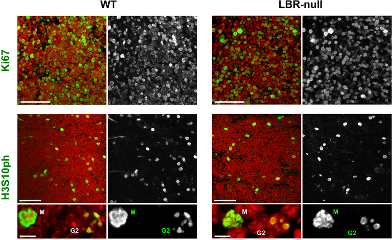
Extended Data Figure 2. The majority of thymocytes are actively cycling cells in both WT (left column) and LBR-null (right column) mice.

Thymus cryosections are immunostained with antibodies for Ki67, a marker of cycling cells, and for phosphorylated H3S10, a marker for G2 and mitotic cells. Note, that in agreement with a seemingly normal immune system of LBR-null mice³¹, the number of cycling thymocytes in their thymuses is comparable to that of WT mice.

M, mitotic cells; G2, cells in mid/late G2. Ki67 staining: projections of 5 μm confocal stacks. H3S10ph staining: projections of 10 μm (for overviews) or 3 μm (for zoomed areas) confocal stacks. Antibodies: mouse anti-H3S10ph (Abcam, ab14955) and rabbit anti-Ki67 (Abcam, ab15580). Immunostaining and microscopy were performed as described in Methods.

Extended Data Figure 3. Quantitative analysis of TADs.

a, Average TADs, based on domain calls from ESC (embryonic stem cells)³². Ticks indicate start and end of TADs. The visual suggestion is that TADs are weakest in rods and strongest in non-rod neurons, with the thymocytes intermediate.

b, TAD strength is weakest in rods and strongest in non-rod neurons. TAD strength is the ratio of average contacts within the TAD (pink triangle on the inset) to average contacts between TADs (blue triangles). TAD strength is calculated separately for each autosome in two replicas. (n=38 chromosomes, centerline is median, box is between lower and upper quartiles, whiskers extend to 1.5 times the interquartile range).

c, Spearman correlation of insulation profiles across multiple mouse cell types (data from references^33,34, first author indicated in row/column label, GEO accession numbers GSE35156, GSE63525), clustered hierarchically.

d, Average insulation profile (Methods) around TAD boundaries called in ESC³². The minimum insulation score of each profile is set to zero. We symmeterize noise by reflecting around the TAD boundary and averaging the reflected and original profiles.

e, Decay of contact probability, P(s), as a function of genomic separation, s. Shaded areas are bounded by P(s) curves for biological replicas. All P(s) curves are normalized to their value at 10kb. For rods, the steeper slope below 1Mb and lack of a rollover in contrast to the other three cell types is indicative of weaker TADs, as in Schwarzer et al.³⁵

f, TAD strength as a function of cell type (columns) and cell type from which TADs are called (rows) (data from references^32,34,35, first author indicated in row/column label, GEO accession numbers GSE98671, GSE63525, GSE93431). Note that rods cluster with cell types with demonstrated weaker TADs. TAD strength is computed differently than in ED Fig. 3b (Methods).

g, Average insulation profile (Methods) oriented around top 10⁴ scoring CTCF motifs. For scoring, we used the FIMO algorithm³⁶, with a position weight matrix for the M1 motif as in Schmidt et al.³⁷ The minimum insulation score of each profile is set to zero, and the CTCF motif points to the left. This provides a TAD-call independent method of inferring TAD strength, given that CTCF is frequently present at the borders of TADs.

h, Snapshot of Hi-Glass³⁸ view of the four data sets, close to the diagonal (chr12:77,538,523–85,180,785 & chr12:79,240,367–82,837,977, 32kb resolution). Rods are almost completely lacking TADs and non-rod neurons have very strong TADs, upon inspection. Datasets can be browsed in a more in-depth fashion on a public server (http://higlass.io/app/?config=JLOhiPILTmq6qDRicHMJqg)

Extended Data Figure 4. Quantitative analysis of territories.

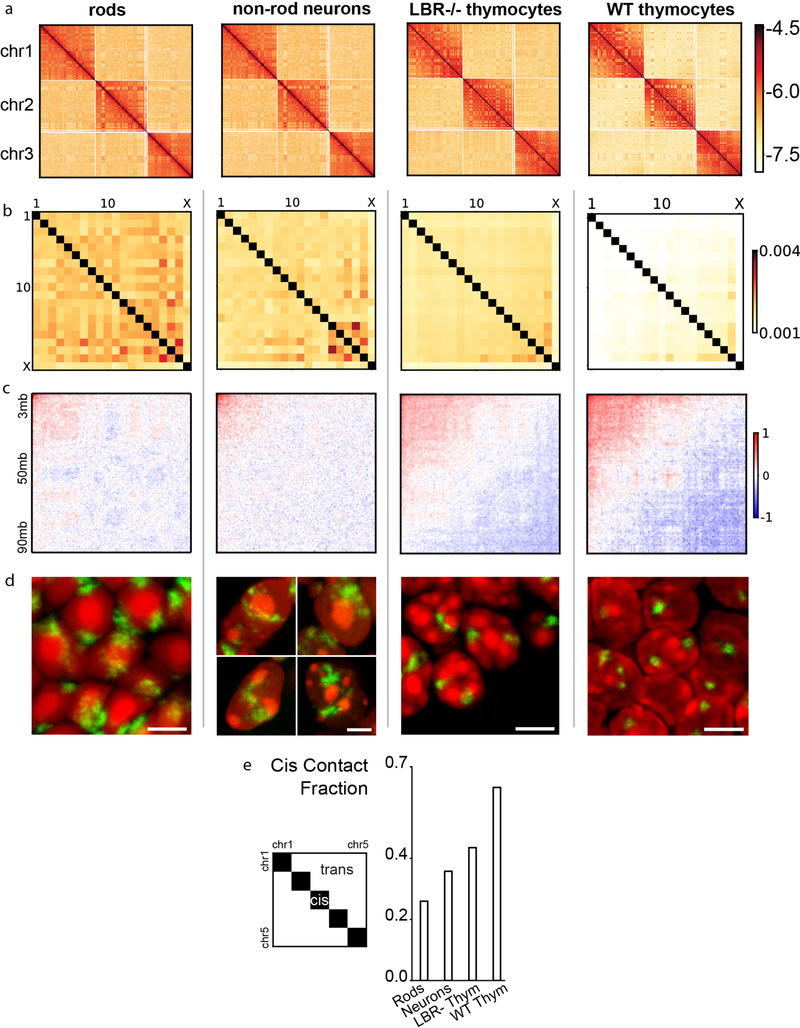
a, Hi-C contact maps for chromosomes 1, 2, and 3 show both a checkerboard pattern in cis (within a chromosome) and trans (between chromosomes), reflecting compartmentalization, and more frequent cis than trans contacts, reflecting chromosome territoriality. Views are shown for the second biological replicate, binned at 500kb.

b, Average number of contacts between pairs of chromosomes. Average cis contacts are much higher than trans contacts. Maps are normalized by their sums.

c, Average contacts in trans. For every unique pair of chromosomes, we average the first 60Mb, binned at 500kb resolution. Maps are normalized to their means, and plotted in log-space. There is evidence of weak enrichment among chromocenter-proximal regions in trans, independent of inversion status.

d, Consistent with the low cis contact fraction revealed by Hi-C, chromosome 11 visualized by FISH (green) has a more diffuse territory in postmitotic rods and non-rod neurons in comparison to cycling thymocytes of both genotypes. Projections of 2 μm confocal stacks; scale bars, 5 μm. The chromosome painting was performed in four independent experiments.

e, Chromosome territoriality, measured as the ratio of cis contacts to cis+trans contacts, is weaker in rods and non-rod neurons in comparison to conventional and inverted thymocytes. The schematic illustrates the compared regions.

i, Scatterplot of compartmentalization and territoriality. The two metrics are not necessarily related.

Extended Data Figure 5. Quantitative analysis of compartments.

a, Saddle plots²² (see Methods) displaying contact frequency enrichment show the extent of compartmentalization across cell types in cis.

b, Spearman correlation of compartment profiles across multiple mouse cell types (data from references^33,39,40, first author indicated in row/column label, GEO accession numbers GSE35156, GSE35519, GSE40173), clustered hierarchically. Spearman’s r(LBR1,WT1)=.95, p<10⁻¹⁰, n=4780; r(LBR1,LBR2)=.98, p<10⁻¹⁰, n=4780; r(WT1,WT2)=.99, p<10⁻¹⁰, n=4780. P-values are from two-sided tests. Positions of compartments are almost exactly the same between thymocytes and LBR−/− thymocytes, approaching that of biological replicas, which allows us to infer that inversion does not change compartment positions per-se.

c-e, Fraction of loci which remain the same comparing two different cell types, as well as fractions of loci switching from B to A and from A to B. The sequence of cell types is taken from the clustering of their compartment profiles.

f, Compartment strength across multiple mouse cell types (calculated separately for each autosome, n=19 for datasets not considered in main text, n=38 for two replicates of main text datasets. Centerline is median, box is between lower and upper quartiles, whiskers extend to 1.5 times the interquartile range).

Extended Data Figure 6. Exploring the space of model classes reveals only a small fraction can reproduce the inverted nuclear geometry.

a, Even the second-best group of models do not display the ring-like structure characteristic of the inverted nucleus (the eight models, indicated in pink, after the 8 best models shown in the main text, indicated in gold). Densities are computed from 50 simulated configurations.

b, In agreement with Flory-Huggins theory, we find that if the cross-type attraction (e.g. A-B) is greater than both of the same-type attractions (A-A and B-B), the two monomer types will not segregate. For models 8, 11, and 15, this is true of both A-B and B-C terms, and as expected, there is mixing between A and B monomers, and B and C monomers in simulation. Similarly, models 9 and 10 have mixed A and C monomers and high A-C attraction; models 12 and 13 have mixed A and B monomers and higher A-B attraction; and model 14 has mixed B and C monomers, with high B-C attraction.

c, Averaging the parameter orders of the second best models classes reveals that they depart from the best-performing models, in aggregate.

d, We illustrate particular models with strong euchromatic interactions to show that such models do not compare well with microscopy, even on a quantitative level. In particular, we show the four worst-performing models (pink dots, models 716–719), all of which are characterized by strong euchromatic interactions (b). We also show the best performing model with AA as its strongest interaction (gold dot, model 250) and the best performing model with AA as its second strongest interaction (gold dot, model 61). Neither of these models compare well with experimental microscopy results. Densities are computed from 50 simulated configurations.

e, All of the poorly-performing models discussed above are characterized by strong AA interactions.

f, Averaging the worst four models shows that they are characterized by strong AA interactions.

Extended Data Figure 7. The heterochromatin-dominated model is robust to perturbations and outperforms a variety of alternative models.

a, Adding in a fraction of B monomers attracted to the lamina, in analogy to trace amounts of peripheral heterochromatin in rods⁴¹, does not significantly change agreement with microscopy. Representative configurations as this fraction is increased are shown. Boxes indicate density peak distance with whiskers extending to 1.5 times the interquartile range (n=50, number of time points sampled across 3 simulation replicates).

b, Adding in small fractions of A monomers attracted to the lamina (below 20%) does not significantly change the conventional morphology of simulated nuclei. Representative configurations as this fraction is increased are shown. Quantities plotted as in (a). This simulation reflects a potential phenomenon of association between highly transcribed genes and nuclear pores. Of note, we have not observed this phenomenon in nuclei of mouse cells, including rod cells, in which all euchromatin is adjacent to the nuclear lamina (Supplemental Fig. 2). (n=8 simulated chromosomes)

c, Average compartment strength across simulated chromosomes (n=8) as a function of B-B and B-Lam attractions. The zone of parameter space where simulated Hi-C compartment strength agrees with experimental compartment strength is virtually unchanged for simulations with some interior chromocenters, compared to simulations with no interior chromocenters. Representative configurations of each of these models are displayed below. Orange outline indicates regions in parameter space where simulated Hi-C has compartmentalization in agreement with experimental Hi-C data (+/− one standard deviation of the median for WT thymocytes).

d, For BB = .5 and all other parameters as in the main text, increasing the ratio of AA to BB results in worse agreement with microscopy. This is particularly visible above AA/BB = .5. Representative configurations as this fraction is increased are shown. Quantities plotted as in (a). (n=8 simulated chromosomes) Additional models are considered in Supplemental Fig. 6.

Extended Data Figure 8. Chromocenters merge during nuclear inversion and pass through a partially inverted morphology.

a, Distance between chromocenters decreases once interactions with the lamina have been removed, quantitatively showing the fusion of C monomer droplets. To see this, we find the center of mass of the C monomer blocks on each of the eight chromosomes in our simulation. We then compute the average distance between all possible pairs of the eight center of masses, and normalize by the maximum possible total separation in the nucleus, i.e. the diameter of the nucleus times the number of chromosome pairs; light blue lines show individual trajectories, dark blue shows average over trajectories. Following release from the lamina (vertical black line), this metric drops, quantitatively conforming what we see visually in the associated configurations (roman numerals).

b, Following three representative simulations starting from an initial condition where chromosomes are in mitotic-like condensed cylindrical conformations, we find that our inverted nucleus model reaches its equilibrium configuration via a pathway that passes through a state highly reminiscent of the partial inversion seen in LBR-null thymocytes. As a proxy for detailed mechanistic modelling of the complexities of mitotic exit, we begin from cylinders that are randomly oriented, as opposed to aligned. Scale bar, 2 μm.

c, Distance between chromocenters decreases once interactions with the lamina have been removed, while the overall volume of the nucleus shrinks at the same time. Quantities plotted as in (a), with an additional black line for volume decrease relative to initial volume. We see that the qualitative trends in morphology remain the same as in the constant volume case (Fig. 4a).

Extended Data Figure 9. Small chromosome segments faithfully localize to and move together with chromatin of their own compartment during nuclear inversion.

The nuclear positions of short chromosome segments of different gene densities belonging to either A or B compartment were studied using FISH with a cocktail of BAC probes on retinal cryosections at six developmental stages: P0, P6, P13, P21, P28 and adult (AD, 3.5 months). For the analysis of BAC signal distribution, three stages were considered: P0 with conventional nuclei of rod progenitors, P13 with rod nuclei in a transient state of inversion and adult with fully inverted rod nuclei. Cells with conventional nuclear organization in the inner nuclear layer (INL) of adult retina were used as a control. Between 100 and 120 alleles per chromosomal region were analyzed.

a, Immuno-FISH experiment showing how FISH signals were classified according to their localization in the three major nuclear zones - euchromatin (EC), heterochromatin (HC) and constitutive heterochromatin (cHC) (a3; see ¹ for definitions of these three types of chromatin). BAC 12 maps to the most peripheral euchromatic shell of the rod nucleus stained with antiH3K4me3 antibody (a1). This nuclear zone is adjacent to the nuclear periphery and contains the genic part of the mouse genome (see Supplementary Figure S2). BACs 2 and 11 are located in the heterochromatic zone of the nucleus encircling the chromocenter and stained with antiH4K20me3 antibody (a2). Thus, classification of BAC signals based on DAPI staining is justified by immunostaining of histone modifications and enables the signal distribution analysis described in b-d. Top panels show localization of BAC signals (blue, white arrows) and histone modifications (green) in DAPI counterstained nuclei (red). Numbers in the lower left corners indicate the BAC numbers (for their coordinates see Methods). Bottom panels show grey-scale images of DAPI and positions of the BAC signals (red arrows) represented by false-colored mask.

b, c, d, Analysis of BAC signal positions after FISH with BAC cocktail probes mapping to selected chromosome regions. b1, c1, d1, Schematics of the chromosome regions on MMU1, MMU2 and MMU6, respectively. The differentially colored segments differ in their gene content and assignment to either A or B compartment. The striped boxes with numbers below indicate the BACs used for FISH. b2, c2, d2, Graphs showing the distribution of the segments within rod nuclei at the three developmental stages and adult INL cells. The bars represent the proportion of signals in each nuclear zone: adjacent to constitutive heterochromatin (cHC, dark grey), within heterochromatin (HC, light grey) and within euchromatin (EC, white). b3, c3, d3, Schematics, showing typical segment distribution of the studied regions. b4, c4, d4, Representative nuclei after 3-color (b4) or 4-color FISH (c4,d4). The images are maximum intensity projections of short (1.4 – 2 μm) stacks. False colors assigned to segments correspond to the color code used for b1–3, c1–3 and d1–3. The experiment was repeated twice.

For an example of the localization of a single gene and its movement together with chromatin of the A compartment during nuclear inversion, see Supplementary Figure S3.

Extended Data Figure 10. Coalescence of individual chromocenters into a large central chromocenter is irreversible.

a1, Our model predicts that once nuclei invert and all individual chromocenters merge into a single central chromocenter, the reverse process, re-splitting into smaller chromocenters, will not take place after reintroduction of lamina attractions. While we expect B monomers to redistribute to the nuclear lamina, we do not expect C monomers of a single globule to reorganize into smaller globules. In this sense, our model predicts that inversion and formation of the central chromocenter are irreversible.

a2, Simulations of de-inversion of inverted nuclei via the introduction of B-Lam and C-Lam attractions with strengths equal to the optimal B-Lam value from Fig. 3f. Note, that according to our prediction, de-inverted nuclei only partially return to the conventional geometry. Slices with thickness of 5% of the nuclear diameter are shown.

b1, b2, In agreement with the model prediction, de-inverted nuclei do not return to a typical conventional architecture, as can be seen in de-differentiated rods of R7E mice expressing polyQ-expanded ataxin-7 (see Supplementary Figure 5a,b for description of the phenotype). FISH with probes for major satellite repeat (MSR, blue), LINE-rich heterochromatin (red) and SINE-rich euchromatin (green) demonstrates that although euchromatin returns to the nuclear interior (solid arrowheads) and heterochromatin repositions to the lamina (empty arrowheads), a single large chromocenter remains and is typically positioned at the nuclear periphery (b1, arrows). Remarkably, in ca. 30% of the nuclei, the large chromocenter does not relocate to the nuclear periphery but the nuclear lamina (green) makes deep narrow invaginations, contacting the chromocenter (b2, arrows; see also Supplementary Figure 5c). The remaining bulky chromocenter is surrounded by LINE-rich chromatin (empty arrowheads) and is often (71% of nuclei) in contact with the nuclear periphery as a result of nuclear shape deformation (for more examples, see Supplementary Figure 5c). For comparison, the two left columns show conventional nuclei of ganglion cells and inverted rod nuclei from a WT mouse. Images are single optical sections; scale bar, 2 μm. Probes, FISH and microscopy are described in the Methods section. Each experiment was repeated three times.

References

- 1.Solovei I, Thanisch K & Feodorova Y. How to rule the nucleus: divide et impera. Curr. Opin. Cell Biol 40, 47–59 (2016). [DOI] [PubMed] [Google Scholar]
- 2.van Steensel B. & Belmont AS Lamina-Associated Domains: Links with Chromosome Architecture, Heterochromatin, and Gene Repression. Cell 169, 780–791 (2017). [DOI] [PMC free article] [PubMed] [Google Scholar]
- 3.Bonev B. & Cavalli G. Organization and function of the 3D genome. Nat. Rev. Genet 17, 661–678 (2016). [DOI] [PubMed] [Google Scholar]
- 4.Jerabek H. & Heermann DW How chromatin looping and nuclear envelope attachment affect genome organization in eukaryotic cell nuclei. Int. Rev. Cell Mol. Biol 307, 351–381 (2014). [DOI] [PubMed] [Google Scholar]
- 5.Jost D, Carrivain P, Cavalli G. & Vaillant C. Modeling epigenome folding: formation and dynamics of topologically associated chromatin domains. Nucleic Acids Res. 42, 9553– 9561 (2014). [DOI] [PMC free article] [PubMed] [Google Scholar]
- 6.Lee SS, Tashiro S, Awazu A. & Kobayashi R. A new application of the phase-field method for understanding the mechanisms of nuclear architecture reorganization. J. Math. Biol 74, 333–354 (2017). [DOI] [PMC free article] [PubMed] [Google Scholar]
- 7.Di Pierro M, Zhang B, Aiden EL, Wolynes PG & Onuchic JN Transferable model for chromosome architecture. Proc. Natl. Acad. Sci. U. S. A 113, 12168–12173 (2016). [DOI] [PMC free article] [PubMed] [Google Scholar]
- 8.Nuebler J, Fudenberg G, Imakaev M, Abdennur N. & Mirny L. Chromatin Organization by an Interplay of Loop Extrusion and Compartmental Segregation. (2017). doi: 10.1101/196261 [DOI] [PMC free article] [PubMed] [Google Scholar]
- 9.van de Werken HJG et al. Small chromosomal regions position themselves autonomously according to their chromatin class. Genome Res. 27, 922–933 (2017). [DOI] [PMC free article] [PubMed] [Google Scholar]
- 10.Larson AG et al. Liquid droplet formation by HP1α suggests a role for phase separation in heterochromatin. Nature 547, 236–240 (2017). [DOI] [PMC free article] [PubMed] [Google Scholar]
- 11.Strom AR et al. Phase separation drives heterochromatin domain formation. Nature 547, 241–245 (2017). [DOI] [PMC free article] [PubMed] [Google Scholar]
- 12.Machida S. et al. Structural Basis of Heterochromatin Formation by Human HP1. Mol. Cell 69, 385–397.e8 (2018). [DOI] [PubMed] [Google Scholar]
- 13.Ganai N, Sengupta S. & Menon GI Chromosome positioning from activity-based segregation. Nucleic Acids Res. 42, 4145–4159 (2014). [DOI] [PMC free article] [PubMed] [Google Scholar]
- 14.Grosberg AY & Joanny J-F Nonequilibrium statistical mechanics of mixtures of particles in contact with different thermostats. Phys. Rev. E Stat. Nonlin. Soft Matter Phys 92, 032118 (2015). [DOI] [PubMed] [Google Scholar]
- 15.Smrek J. & Kremer K. Small Activity Differences Drive Phase Separation in Active-Passive Polymer Mixtures. Phys. Rev. Lett 118, 098002 (2017). [DOI] [PubMed] [Google Scholar]
- 16.Stevens TJ et al. 3D structures of individual mammalian genomes studied by single-cell Hi-C. Nature 544, 59–64 (2017). [DOI] [PMC free article] [PubMed] [Google Scholar]
- 17.Hilbert L. et al. Transcription establishes microenvironments that organize euchromatin. bioRxiv (2017). doi: 10.1101/234112 [DOI] [Google Scholar]
- 18.Zheng X. et al. Lamins organize the global three-dimensional genome from the nuclear periphery. bioRxiv 211656 (2017). doi: 10.1101/211656 [DOI] [PMC free article] [PubMed] [Google Scholar]
- 19.Solovei I. et al. Nuclear architecture of rod photoreceptor cells adapts to vision in mammalian evolution. Cell 137, 356–368 (2009). [DOI] [PubMed] [Google Scholar]
- 20.Solovei I. et al. LBR and lamin A/C sequentially tether peripheral heterochromatin and inversely regulate differentiation. Cell 152, 584–598 (2013). [DOI] [PubMed] [Google Scholar]
- 21.Eberhart A. et al. Epigenetics of eu-and heterochromatin in inverted and conventional nuclei from mouse retina. Chromosome Res. 21, 535–554 (2013). [DOI] [PubMed] [Google Scholar]
- 22.Imakaev M. et al. Iterative correction of Hi-C data reveals hallmarks of chromosome organization. Nat. Methods 9, 999–1003 (2012). [DOI] [PMC free article] [PubMed] [Google Scholar]
- 23.Ou HD et al. ChromEMT: Visualizing 3D chromatin structure and compaction in interphase and mitotic cells. Science 357, (2017). [DOI] [PMC free article] [PubMed] [Google Scholar]
- 24.Andy Choo KH The Centromere. (Oxford University Press, 1997). [Google Scholar]
- 25.Rubinstein M. & Colby RH Polymer physics. 23, (Oxford University Press; New York, 2003). [Google Scholar]
- 26.Biggs R, Stephens AD, Liu P. & Marko JF Effects of altering histone posttranslational modifications on mitotic chromosome structure and mechanics. doi: 10.1101/423541 [DOI] [PMC free article] [PubMed] [Google Scholar]
- 27.Helmlinger D. et al. Glutamine-expanded ataxin-7 alters TFTC/STAGA recruitment and chromatin structure leading to photoreceptor dysfunction. PLoS Biol. 4, e67 (2006). [DOI] [PMC free article] [PubMed] [Google Scholar]
- 28.Tang S-J Chromatin Organization by Repetitive Elements (CORE): A Genomic Principle for the Higher-Order Structure of Chromosomes. Genes 2, 502–515 (2011). [DOI] [PMC free article] [PubMed] [Google Scholar]
- 29.Rosa A. & Everaers R. Structure and dynamics of interphase chromosomes. PLoS Comput. Biol. 4, e1000153 (2008). [DOI] [PMC free article] [PubMed] [Google Scholar]
- 30.Abdennur N. & Mirny L. Cooler: scalable storage for Hi-C data and other genomicallylabeled arrays. BioRxiv (2019). [DOI] [PMC free article] [PubMed] [Google Scholar]
Methods and ED References
- 31.Shultz LD Mutations at the mouse ichthyosis locus are within the lamin B receptor gene: a single gene model for human Pelger-Huet anomaly. Hum. Mol. Genet 12, 61–69 (2003). [DOI] [PubMed] [Google Scholar]
- 32.Nora EP et al. Targeted Degradation of CTCF Decouples Local Insulation of Chromosome Domains from Genomic Compartmentalization. Cell 169, 930–944.e22 (2017). [DOI] [PMC free article] [PubMed] [Google Scholar]
- 33.Dixon JR et al. Topological domains in mammalian genomes identified by analysis of chromatin interactions. Nature 485, 376–380 (2012). [DOI] [PMC free article] [PubMed] [Google Scholar]
- 34.Rao SSP et al. A 3D map of the human genome at kilobase resolution reveals principles of chromatin looping. Cell 159, 1665–1680 (2014). [DOI] [PMC free article] [PubMed] [Google Scholar]
- 35.Schwarzer W. et al. Two independent modes of chromatin organization revealed by cohesin removal. Nature 551, 51–56 (2017). [DOI] [PMC free article] [PubMed] [Google Scholar]
- 36.Grant CE, Bailey TL & Noble WS FIMO: scanning for occurrences of a given motif. Bioinformatics 27, 1017–1018 (2011). [DOI] [PMC free article] [PubMed] [Google Scholar]
- 37.Schmidt D. et al. Waves of retrotransposon expansion remodel genome organization and CTCF binding in multiple mammalian lineages. Cell 148, 335–348 (2012). [DOI] [PMC free article] [PubMed] [Google Scholar]
- 38.Kerpedjiev P. et al. HiGlass: Web-based Visual Exploration and Analysis of Genome Interaction Maps. bioRxiv 121889 (2018). doi: 10.1101/121889 [DOI] [PMC free article] [PubMed] [Google Scholar]
- 39.Zhang Y. et al. Spatial organization of the mouse genome and its role in recurrent chromosomal translocations. Cell 148, 908–921 (2012). [DOI] [PMC free article] [PubMed] [Google Scholar]
- 40.Lin YC et al. Global changes in the nuclear positioning of genes and intra- and interdomain genomic interactions that orchestrate B cell fate. Nat. Immunol 13, 1196–1204 (2012). [DOI] [PMC free article] [PubMed] [Google Scholar]
- 41.Kizilyaprak C, Spehner D, Devys D. & Schultz P. In vivo chromatin organization of mouse rod photoreceptors correlates with histone modifications. PLoS One 5, e11039 (2010). [DOI] [PMC free article] [PubMed] [Google Scholar]
- 42.Solovei I. Fluorescence in situ Hybridization (FISH) on Tissue Cryosections. in Methods in Molecular Biology 71–82 (2010). doi: 10.1007/978-1-60761-789-1_5 [DOI] [PubMed] [Google Scholar]
- 43.Eberhart A, Kimura H, Leonhardt H, Joffe B. & Solovei I. Reliable detection of epigenetic histone marks and nuclear proteins in tissue cryosections. Chromosome Res. 20, 849–858 (2012). [DOI] [PubMed] [Google Scholar]
- 44.Cremer M. et al. Multicolor 3D fluorescence in situ hybridization for imaging interphase chromosomes. Methods Mol. Biol 463, 205–239 (2008). [DOI] [PubMed] [Google Scholar]
- 45.Walter J. et al. Towards many colors in FISH on 3D-preserved interphase nuclei. Cytogenet. Genome Res 114, 367–378 (2006). [DOI] [PubMed] [Google Scholar]
- 46.Feodorova Y, Koch M, Bultman S, Michalakis S. & Solovei I. Quick and reliable method for retina dissociation and separation of rod photoreceptor perikarya from adult mice. MethodsX 2, 39–46 (2015). [DOI] [PMC free article] [PubMed] [Google Scholar]
- 47.Cohen TV et al. The lamin B receptor under transcriptional control of C/EBPepsilon is required for morphological but not functional maturation of neutrophils. Hum. Mol. Genet 17, 2921–2933 (2008). [DOI] [PMC free article] [PubMed] [Google Scholar]
- 48.Naumova N. et al. Organization of the mitotic chromosome. Science 342, 948–953 (2013). [DOI] [PMC free article] [PubMed] [Google Scholar]
- 49.Heinz S. et al. Simple combinations of lineage-determining transcription factors prime cis-regulatory elements required for macrophage and B cell identities. Mol. Cell 38, 576–589 (2010). [DOI] [PMC free article] [PubMed] [Google Scholar]
- 50.Flyamer IM et al. Single-nucleus Hi-C reveals unique chromatin reorganization at oocyte-to-zygote transition. Nature 544, 110–114 (2017). [DOI] [PMC free article] [PubMed] [Google Scholar]
- 51.Crane E. et al. Condensin-driven remodelling of X chromosome topology during dosage compensation. Nature 523, 240–244 (2015). [DOI] [PMC free article] [PubMed] [Google Scholar]
- 52.Eastman P. et al. OpenMM 4: A Reusable, Extensible, Hardware Independent Library for High Performance Molecular Simulation. J. Chem. Theory Comput 9, 461–469 (2013). [DOI] [PMC free article] [PubMed] [Google Scholar]
- 53.Eastman P. et al. OpenMM 7: Rapid development of high performance algorithms for molecular dynamics. PLoS Comput. Biol 13, e1005659 (2017). [DOI] [PMC free article] [PubMed] [Google Scholar]
Associated Data
This section collects any data citations, data availability statements, or supplementary materials included in this article.
Supplementary Materials
Data Availability Statement