Supervised and unsupervised machine learning for automated scoring of sleep–wake and cataplexy in a mouse model of narcolepsy

Abstract

Despite commercial availability of software to facilitate sleep–wake scoring of electroencephalography (EEG) and electromyography (EMG) in animals, automated scoring of rodent models of abnormal sleep, such as narcolepsy with cataplexy, has remained elusive. We optimize two machine-learning approaches, supervised and unsupervised, for automated scoring of behavioral states in orexin/ataxin-3 transgenic mice, a validated model of narcolepsy type 1, and additionally test them on wild-type mice. The supervised learning approach uses previously labeled data to facilitate training of a classifier for sleep states, whereas the unsupervised approach aims to discover latent structure and similarities in unlabeled data from which sleep stages are inferred. For the supervised approach, we employ a deep convolutional neural network architecture that is trained on expert-labeled segments of wake, non-REM sleep, and REM sleep in EEG/EMG time series data. The resulting trained classifier is then used to infer on the labels of previously unseen data. For the unsupervised approach, we leverage data dimensionality reduction and clustering techniques. Both approaches successfully score EEG/EMG data, achieving mean accuracies of 95% and 91%, respectively, in narcoleptic mice, and accuracies of 93% and 89%, respectively, in wild-type mice. Notably, the supervised approach generalized well on previously unseen data from the same animals on which it was trained but exhibited lower performance on animals not present in the training data due to inter-subject variability. Cataplexy is scored with a sensitivity of 85% and 57% using the supervised and unsupervised approaches, respectively, when compared to manual scoring, and the specificity exceeds 99% in both cases.

Statement of Significance.

This is, to the best of our knowledge, the first set of algorithms created to specifically identify pathological sleep in narcoleptic mice. Currently available sleep-scoring algorithms are trained on wild-type animals with normal sleep/wake behavior and exhibit low accuracies for scoring pathological sleep. Our supervised and unsupervised classifiers provide valuable tools that can greatly facilitate and expedite behavioral-state-scoring in narcoleptic mice. Both methods successfully score EEG/EMG data and can be manually corrected as necessary. All algorithms implemented in this work (including example datasets) can be made available upon request.

Introduction

Narcolepsy type 1 (narcolepsy with cataplexy, NT1) is a neurological disorder characterized by sleep–wake fragmentation, intrusion of rapid-eye-movement sleep (REMS) during wake, and cataplexy—an abrupt loss of muscle tone typically triggered by strong emotion. Narcolepsy with cataplexy results from an autoimmune-mediated loss of orexin/hypocretin neurons in the hypothalamus, affecting about 1:2000 people at any age. There is no cure for narcolepsy and morbidity results from excessive daytime sleepiness, nocturnal sleep disturbance, cataplexy, and medication side-effects.

Currently validated rodent models of NT1 provide a means of exploring neurobiology and novel treatments for this disorder [1–5]; however, many experimental paradigms using NT1 rodent models laboriously manually score vigilance states from videography and/or electrophysiological data. This slow process is thus the main bottleneck in executing such studies. At present, automated sleep-scoring algorithms that use EEG/EMG have not been validated in narcolepsy models [6–8] and are typically restricted to supervised approaches (i.e. requiring previously scored data on which to train) [9–11]. As narcolepsy remains one of the most intensively studied sleep disorders, developing approaches to analyze abnormal patterns of sleep–wake, including cataplexy, will alleviate the experimental bottleneck of manual scoring and demonstrate a proof-of-principle for the automatic scoring of models of sleep disorders.

In general, the task of classification within traditional supervised machine learning requires a significant amount of data pre-processing, as well as human-expert selection of a number of potential features that could be useful for classification. Modern deep learning, relying on multi-layer neural networks, offers an alternative approach based on the concept of feature learning [12] (although it does not obviate the need for judicious filtering to avoid aliasing and other errors). Given a family of transformations, feature learning allows a mapping of the input space to a feature space that encodes the relevant information for the task at hand. Feature learning is particularly manifested within a class of artificial neural networks, called convolutional neural networks (CNNs). In the context of supervised learning, CNNs are trained to search for patterns through a process of network training in which a collection of filters is constructed, making learning more computationally tractable. The main limitation of the supervised learning approach is that it requires accurately labeled examples from which to learn.

In contrast, unsupervised learning, on the other hand, addresses the task of identifying any underlying structure, similarities, or patterns within unlabeled data. Two complementary components of unsupervised learning are manifold learning, which is directly related to data dimensionality reduction, and clustering, which groups together data of high similarity.

With respect to previously published literature, our supervised approach consisting of CNNs exhibits some similarities with a recently published neural network architecture trained on several very large cohorts of human NT1 data [12]. Similar approaches based on CNNs, leveraging the availability of large datasets, have become increasingly popular in other sleep-related applications as well, such as arousal detection [13]. With a large dataset from thousands of patients, one would be able to train a far more complicated CNN structure than the one proposed in our work, with trainable parameters in the order of millions. The objective then is not to perform well on a given, particular patient, but rather to obtain a single, universal classifier with high, robust performance across a multitude of test subjects. Because the data come from thousands of patients, a sophisticated network architecture can take into account and be made resistant to inter-patient variability. Instead, in our work, we aimed to develop a set of tools useful for animal sleep labs that may seek to analyze data from a smaller number of subjects. While we still employed deep CNNs, there are some significant differences: we developed a lower-capacity (much smaller number of trainable parameters) neural network architecture that is geared toward small dataset sizes, and focused on performance by subject (i.e. when each classifier is customized for the particular subject whose data it is being trained on). Subject-customized CNN models generalize well on unseen data, as long as they stem from an animal whose data were provided during training. This approach is tailored to an unmet need for the more efficient processing of large amounts of data, even if this has been generated from small groups of animal subjects. With respect to the unsupervised method, some similarities are present with the Fully Automated Sleep sTaging method via EEG/EMG Recordings (FASTER) algorithm [8], which uses Principal Component Analysis (PCA, a linear dimensionality reduction method) followed by clustering. The PCA dimensionality reduction component is substituted in our work with t-Distributed Stochastic Neighbor Embedding (t-SNE) [14], a nonlinear and more powerful method than PCA, which may offer an advantage in datasets where a low-dimensional representation that exhibits separation into clusters is difficult to obtain. Another relevant approach is the SCOPRISM open source software [15], a relatively simple algorithm relying on only two features, namely EEG θ − ∆ ratio and EMG (root mean square).

In this work, we compare both supervised and unsupervised learning approaches applied to the scoring of sleep, wake, and cataplexy in an animal model of narcolepsy. Specifically, we propose a CNN classifier that learns to distinguish states using the raw neural time series recording as input. We benchmark the proposed CNN classifier against Support-Vector Machines (SVMs), which were extremely popular at the time of their initial development (1990s), and are still considered as a standard approach that is very effective in many practical applications [16].

We then propose an unsupervised learning algorithm that uses frequency domain information, performs dimensionality reduction using t-SNE first, and then clusters the reduced dimensionality data into groups using Density-Based Spatial Clustering of Applications with Noise (DBSCAN). These groups were hypothesized to correlate with behavioral states, and match at a high percentage with human-expert labels, despite the latter being hidden from the algorithm. The proposed unsupervised approach is benchmarked against the published SCOPRISM algorithm.

Materials and Methods

This study was approved by the Institutional Animal Care and Use Committee (IACUC) of Emory University and was performed in accordance with the National Institutes of Health Guide for the Care and Use of Laboratory Animals. All algorithms implemented in this work (including example datasets) can be made available via the Google Colab environment upon request, and are capable of running through a simple web browser (no installation of software necessary).

Mice

Orexin/ataxin-3 hemizygous transgenic narcoleptic mice (HCRT-MJD 1Stak, backcrossed to C57Bl6J, The Jackson Laboratory; n = 7, 6 females, adult aged 3–6 months), and wild-type mice (C57Bl6J, The Jackson Laboratory, n = 7, 2 females, aged 3–6 months) were used for all experiments. Genotypes of all subjects were confirmed by polymerase chain reaction with DNA primers as previously described [4]. Phenotype of transgenic mice were further confirmed in all narcoleptic subjects by nocturnal infrared videography of individual subjects and expert review for presence of cataplexy behavior as previously described [5].

Following anesthesia induction using isoflurane, mice were head-fixed in a stereotaxic frame (Kopf Instruments) and implanted with the following: two stainless steel EMG pads (Catalog #E363/76//NS/SPC, 0.125”, 50 mm, Plastics1, Preclinical Research Components) in neck muscle for EMG recording; and two stainless steel screws (Catalog #8403, 0.10” electrode with wire lead, Pinnacle Technology, Inc.) at brain surface for surface frontal–contralateral–parietal EEG recording (Bregma + 1.20 mm, right 2.20 mm, and Bregma −3.00 mm, left 2.50 mm, respectively), and one grounding screw (Bregma −7.30 mm). Electrodes were soldered to a Pinnacle Technology, Inc. headmount (Catalog #8431S-M). Dental cement (3M Ketac Cem Aplicap Capsule Permanent Glass Ionomer Luting Cement) was applied to hold instrumentation. Following surgery, mice were individually housed in clear acrylic cages under temperature-, humidity-, and light-controlled conditions (12-h light–dark schedule) with ad libitum food and water. After 2 days of recovery, the affixed headmount was connected to a custom preamplifier (Catalog #8406, ‘”SL” configuration, Pinnacle Technology, Inc). Mice recovered for 7 days before recordings began.

Data collection

Time-locked EEG, EMG, and infrared video of freely behaving mice were simultaneously recorded using the aforementioned custom head-stage preamplifier and a standard acquisition system (Catalog #8408, Pinnacle Technology, Inc.). EEG/EMG were acquired at a 2 kHz sample rate and band-pass filtered online at 0.5 Hz high pass (hardware resistor-capacitor) and 1 kHz low pass (digital), with a preamplifier gain of 100. Data from wild-type mice were provided from the Pedersen lab and were acquired using Spike 2 software, Version 9.04a, Cambridge Electronic Design, Cambridge UK) in conjunction with Pinnacle preamplifier (8406-SE31M) and an analog adapter (8442-PWR-K).

Expert behavioral-state scoring

Rodent sleep was manually scored in 10-s-epochs (a duration typical in rodent sleep studies [2]) in Spike2 (Cambridge Electronic Design, Ltd.) by applying standard criteria for nonrapid eye movement sleep (N), rapid eye movement sleep (R), wakefulness (W), and cataplexy (C), using a combination of EEG, EMG, and video as described previously [17]. Cataplexy was defined as meeting all of the following criteria for at least 10 seconds: (1) abrupt cessation of purposeful waking activity (i.e. eating, vigorous grooming, and ambulating), (2) relative nuchal atonia, (3) increased 7–8 Hz (theta) power in frontal–contralateral–parietal EEG, and (4) relative immobility throughout the episode. Non-REM sleep was defined by 2–3 Hz (delta) predominance in EEG, attenuation of EMG, and behaviorally preceded by typical sleep preparation (i.e. quiet grooming, body/tail curling). REM sleep was defined as theta predominance and relative nuchal atonia preceded by non-REM sleep. If an epoch consisted of more than one state, the predominant state (≥5 s) was scored.

Machine learning methods

Supervised learning—CNN

The core concept behind neural networks is a cascade of layers featuring nonlinear processing units. The output of each layer is fed as an input to the next layer, thus undergoing some transformation. During the training phase of the network, the transformation parameters are altered to best capture the relationship between the input and output data presented to the network. In particular, for the task of multiclass classification, the neural network is merely a universal function approximator that performs the assignment

$${\displaystyle \begin{array}{l}{\displaystyle y=F(x;\theta )}\end{array}}$$

wherein $x$ is the input (neural time series data) and θ are the trainable network parameters. The output, $y$ is a 3-dimensional vector that takes values in the interval 0 to 1 and denotes a probability distribution (or “match percentage”) of the sample x to each of the three classes (W, N, and R). The generic architecture of a CNN is depicted in Figure 1.

Figure 1.

Supervised learning—the CNN architecture. An input sample consists of a 2-s-long segment of EEG/EMG. The sample is fed to the network which then outputs a probability distribution (match percentage) over classes, as shown in example.

Due to a relatively limited amount of data used for training (compared to that available in large cohort studies), we had to exercise caution in avoiding overfitting—a phenomenon in which the neural network is fitted to perfectly match the training data but fails to generalize on test data. This was accomplished by keeping the number of the CNN trainable parameters relatively low (around 70,000 as opposed to several million, which is typically the case in large-scale deep learning applications), as well as implementing overfitting counter-measures such as batch normalization [18], dropout [19], and early stopping (i.e. stopping the training of the network prematurely, before it enters the overfitting regime; this is done by tracking its performance after each epoch of training on a separate, withheld validation set). The CNN architecture in this work consisted of eight convolution layers (number of filters: [16,16,16,16,32,32,64,64], filter size 1 × 5), 5 max-pooling layers (window of 2) and 2 dense layers of 256 and 128 (artificial) neurons, respectively. All activations were rectified linear units (ReLUs), except for the output layer, in which a softmax activation was used for multiclass classification. While this network architecture is loosely inspired by typical CNNs for image recognition tasks, there are some key differences, as we do not perform convolution across channels (i.e. convolving EEG and EMG together) and furthermore the total number of parameters is kept low due to the relatively small size of our datasets. The network was trained on the categorical cross-entropy objective function for 200 epochs using the Adam optimizer [20] with a batch size of 16 samples. All implementation used Keras [21] and TensorFlow [22] libraries.

Given labeled segments of neural activity, we constructed a classifier that learns to categorize a segment into one of three classes: Wake (W), Non-REM (N), and REM (R). Cataplexy (C) is not discriminated from R until a post-processing layer is applied to the output of the artificial neural network that distinguishes C as a fourth class (see Automatic Scoring of Cataplexy Section). All datasets were prepared by downsampling the EEG at 100 Hz (using the resample command, MATLAB R2018a, The MathWorks, Inc., Natick, MA) and dividing the epochs into 2-s bins. The input to the CNN consisted of the separate EEG and EMG time-series with a 2-channel × 200-sample input for each data sample, and convolution was performed only across the second axis (i.e. across time, not across channel). The choice of a 2-s window for the CNN input was made after we empirically determined it to be advantageous to average the CNN output of several 2-s inputs in order to get a label of 10 s duration, rather than to feed the entire 10-s input to the CNN (as a 10-s long input would have the dimensionality of 2 × 1000). As the manual scoring window is 10 s, the actual behavioral state transition is not necessarily time-locked with the assigned label transition. Thus, to avoid contaminating the classes with state-transition periods, epochs at the end of one state and beginning of another state were discarded during training. Because labels within a dataset are unbalanced and depend on time of day/light cycle (typically around 55% W, 35% N, 8% R, and 2% C, averaged over a 24-h period), a balanced dataset was created for training by utilizing 80% of the R data and adding an equal number of data from the rest of the classes (except for C, which was excluded as a class from training) via random subsampling. Thus, approximately 15% of the total dataset was used for training, leaving the rest for validation. Separate datasets were used exclusively for testing.

To generate model-predicted labels, the dataset is streamed through the trained classifier in a 2-s window, with 1-s step, thus generating a classifier output every second—a vector of probability distributions over states. Every 10 s (an arbitrary interval used by the experts to score files; we used the same interval for the algorithm in order to compare the algorithm’s output to the expert scores), the average probability of each state within that time interval is calculated, and the state with the highest mean probability obtains the label for that scoring interval.

Supervised learning—SVM

An SVM is a classifier that aims to separate classes by constructing a decision boundary where data from each class lie at a maximum margin from it. The data samples most closely located to the decision boundary form the basis of the boundary’s construction and are called support vectors. In contrast to our CNN approach, which acts directly on the raw time series signal, SVMs act on features that are calculated from the time series. Further, the class assignment using SVMs is “hard” rather than probabilistic (as it is the case for CNNs), meaning that the output of the SVM classifier is simply the class assignment itself and carries no information about uncertainty in the assignment, or similarity to other classes.

For dataset preparation, the EEG time series data were divided into segments of 10 s each. The power spectrum in the frequency range 1–50 Hz with 1 Hz resolution was calculated via multitapers using the mtspectrumc command of the Chronux [23] MATLAB toolbox, yielding a total of 49 frequency bins, and each value normalized by the total power in the entire 1–50 Hz range. For the EMG channel, we extracted the signal variance within each 10-s-segment, normalized the values into zero mean, and divided by 4 times their standard deviation. Thus, concatenating the features of the EEG/EMG, each particular sample consists of a 50-dimensional vector. As is customary in supervised learning, we separated the dataset of interest into training, validation, or testing subsets. and balanced the training dataset using the same procedure as described in the previous section.

Unsupervised learning (tSNE+DBSCAN)

In contrast to classification using supervised learning, which requires examples (labeled data) from which to learn, unsupervised learning investigates the presence of underlying structure, similarities, or patterns within the data without considering labels. Our proposed approach for unsupervised learning consists of two components, which address two distinct tasks. The first component is manifold learning, which is a form of nonlinear dimensionality reduction. The fundamental idea behind manifold learning is that the dimensionality of many datasets is only artificially high, and that data can be sufficiently represented in a space of much lower dimensionality. We expected that the 50 dimensions of the input vector (see Supervised Learning—SVM Section) are highly redundant and could likely be reduced to two dimensions.

The second component of the proposed approach is clustering, the process of separating the transformed data into groups of high similarities. There is a wide range of clustering methods available (e.g. the K-means algorithm); for the present application, however, we found the Density-Based Spatial Clustering of Applications with Noise (DBSCAN) [24] algorithm to be the most successful (DBSCAN outperformed both the K-means and the spectral clustering algorithm in recovering behavior-related clusters in all our datasets.). The proposed unsupervised learning approach is summarized in Figure 2. All algorithms were implemented using the sklearn [25] Python library.

Figure 2.

Unsupervised learning—An input sample consists of a 10-s-long segment of EEG/EMG. The EEG is transformed into the frequency domain via Fast Fourier Transform (FFT) and is fed along with the EMG variance (Var) in the t-SNE algorithm, which reduces the dimensionality of the input vector from 50 to 2. Clustering is then performed using the DBSCAN algorithm.

As previously described, unsupervised learning does not require data to be separated into training, validation, and testing subsets. Therefore, we applied the same procedure as described in Supervised Learning—SVM Section on the entire dataset of interest (without balancing classes).

Note that the distinction in the way data are presented to each algorithm (time-domain data for the CNN, as opposed to frequency domain data for the SVM and the unsupervised approach) is a direct consequence of the algorithm’s characteristics. CNNs are by construction designed to search for patterns/features in the raw signal. The time–series data are fed through the convolutional layers of the CNN, which act as trainable filter banks to extract features; these features are then fed in the final two hidden layers of the CNN (which are fully connected as opposed to convolutional) for the final classification. In contrast, SVMs and the unsupervised approach do not act on raw time–series, but instead on some set of features that needs to be extracted from the signal. That is why we use spectral information in this case.

Automatic scoring of cataplexy

Cataplexy was scored in a post-processing layer in which the temporal ordering of each class (i.e. W, N, R) was taken into account, and is henceforth referred to as cataplexy scoring layer (CSL). The input to the CSL is a sequence of labels, obtained from either the supervised or the unsupervised approach, and the output is a modified sequence of labels of the same length. The modifications to the labels are done according to the following six physiological/algorithmic rules that follow from consensus criteria [17]:

1. Extended Wake Prerequisite: A bout of REM sleep can only be labeled as cataplexy when it is preceded by at least 4 epochs (40 s) of wakefulness. This rule is enforced to ensure that labels following a brief arousal during a normal sleep bout (e.g. an arousal during REM sleep) are not labeled as cataplexy.

2. Direct Cataplexy: REM that directly follows wake is labeled as cataplexy.

3. Indirect Cataplexy: A sleep bout that begins with less than or equal to 3 epochs (30 s) of non-REM sleep (potentially including brief arousals) and is subsequently followed by REM sleep is labeled as cataplexy.

4. Prevent Cataplexy to REM Transition: If a cataplexy label is followed by a REM label, the latter is labeled as cataplexy. This rule propagates the cataplexy label on a sequence of REM labels once the first label of the sequence has been identified as cataplexy according to either one of the previous three rules.

5. Brief Arousals/Non-REM during Cataplexy: If a brief arousal or non-REM intrusion (less than or equal to 2 epochs, i.e. 20 s) occurs during a cataplexy bout, sleep epochs (N, R) in the entire bout are labeled as cataplexy (i.e. are not subject to Rule 1).

6. Drowsiness Correction: If a sleep bout begins with up to 3 epochs (30 s) of cataplexy but is then followed by at least 3 epochs (30 s) of non-REM sleep, the cataplexy is relabeled as non-REM. This is a correction to account for transitional periods, drowsiness, and possible sleep-onset REM in the beginning of a normal sleep bout that is sometimes erroneously identified as cataplexy by the algorithm.

We note that the order in which those rules are enforced in the process of modifying the labels is critical, and that some rules must be applied more than once. The operations that constitute the CSL and their order of application are summarized in Algorithm 1; in short, we applied Rule 2 and Rule 3 under the condition of Rule 1, then Rule 4, Rule 5, Rule 4 again, and finally Rule 6.

Algorithm 1.

The Cataplexy Scoring Layer takes the 3-class labels from any of the presented approaches as input and outputs 4-class labels that include cataplexy by applying the rules of Automatic Scoring of Cataplexy section.

Performance metrics

Mean accuracy

Mean accuracy is defined as the percentage of agreement between the model-predicted labels and those labeled by human experts.

Mean confidence (CNN only)

The mean probability for each scoring interval corresponds to the confidence of the classifier for the predicted label in that particular scoring interval. The mean classifier confidence is a metric of how “certain” the classifier is about its predictions for the entire dataset and is calculated by averaging all confidence values for each scoring interval.

Sensitivity/specificity/precision/F1-score

Due to the fact that the cataplexy label occurs infrequently in the data (approximately 2% of the total labels, with some datasets containing <0.05%), the accuracy of the proposed methods in detecting cataplexy can be obscured. To this end, we additionally report the sensitivity, specificity, precision, and F1-score metrics for cataplexy labels. They are defined as follows:

$${\displaystyle \begin{array}{l}{\displaystyle Sensitivity=\frac{TP}{TP+FN}}\end{array}}$$

$${\displaystyle \begin{array}{l}{\displaystyle Specificity=\frac{TN}{FP+TN}}\end{array}}$$

$${\displaystyle \begin{array}{l}{\displaystyle Precision=\frac{TP}{TP+FP}}\end{array}}$$

$${\displaystyle \begin{array}{l}{\displaystyle F1=\frac{2TP}{2TP+FP+FN}}\end{array}}$$

where the quantities TP, FP, TN, and FN stand for the counts of true positives, false positives, true negatives, and false negatives, respectively.

Three-class vs. four-class

The results are reported in two formats: “3-class” and “4-class.” Each classifier described above yields labeled data in a 3-class format (W, N, R). To obtain data in four classes (i.e. include cataplexy as a state), the CSL, which takes the temporal order of samples into account, is applied to the output of interest. Although we are interested detecting cataplexy, we also report 3-class accuracy values in order to compare our algorithm’s output with the SCOPRISM software [15].

Results

Channel contributions to CNN performance

To address the relative contribution of EEG versus EMG for classification using our CNN method, we considered: (a) EEG only, (b) EMG only, and (c) both. For each animal, a CNN classifier was trained on ~15% of 24 h of data from day 1 (D1) and tested on 24 h of data from day 2 (D2). The mean 4-class accuracy for each of the cases are given in Figure 2. A representative example of the output (match percentages and predicted labels) of the channels is depicted in Figure 3. As shown, the EEG channel clearly differentiated between sleep states but had difficulty distinguishing between wake and REM sleep (Figure 3, middle), while the EMG channel distinguished between wake and sleep but poorly separated sleep states (Figure 3, top). When the EEG/EMG channels were combined, the best classification of states was resulted (Figure 3, bottom, see also Figure 4), and both channels were used subsequently.

Figure 3.

Example recording segment (ATA312) that is streamed through the trained CNN classifier. The figure shows a comparison between classifiers relying only on EMG data (top), only on EEG data (middle), and on both EEG/EMG (bottom). HL: human expert label; PL: predicted label; Conf: prediction confidence. Colors blue, red, and green correspond to W, N, and R, respectively. Cataplexy is not represented in this example segment.

Figure 4.

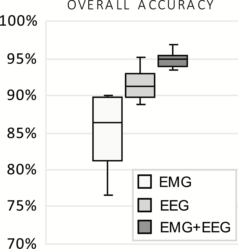
Mean four-class accuracy for the predicted labels of the CNN relying on EEG only, EMG only, and their combination for narcoleptic mice, n = 7. Each classifier is trained on Day 1; results shown are from test sets Day 2 and compared against manual scores.

CNN classifier generalization across animals

We investigated whether a single CNN classifier could be trained to classify labels on datasets originating from multiple animals and be generalized to animals whose data were not included in the classifier training (cross-subject generalization). To address this question, we trained a classifier on approximately 15% of the D1 data pooled from three animals (ATA289, ATA299, and ATA302). The trained classifier was then tested on datasets withheld from training (D2) of the same three animals, in addition to two datasets (D1 and D2) from four novel animals (ATA254, ATA287, ATA301, and ATA312). Note that all the animals used for the study of this Section were narcoleptic, and that the animal group partitioning was done randomly. The results are summarized in Table 1.

Table 1.

Classifier generalization

Animal/ recording	4-Class accuracy (%)	Confidence (%)	Cohen’s kappa
Group I: Training data (~15%)
ATA289/D1	93.5	84.3	0.89
ATA299/D1	95.0	87.4	0.91
ATA302/D1	93.6	87.4	0.89
Average Group I	94.0	86.4	0.90
Group II: Test data—familiar animals
ATA289/D2	92.9	82.5	0.88
ATA299/D2	93.1	86.8	0.88
ATA302/D2	93.6	87.5	0.89
Average Group II	93.2	85.6	0.88
Group II: Test data—novel animals
ATA254/D1	90.2	81.4	0.82
ATA254/D2	88.7	81.4	0.80
Average ATA254	89.5	81.4	0.81
ATA287/D1	63.0	82.5	0.44
ATA287/D2	71.8	82.5	0.54
Average ATA287	67.4	82.5	0.49
ATA301/D1	88.4	82.9	0.80
ATA301/D2	85.8	82.2	0.75
Average ATA301	87.1	82.6	0.78
ATA312/D1	85.4	86.3	0.73
ATA312/D2	92.2	88.9	0.86
Average ATA312	88.8	87.6	0.80

Single classifier trained on multiple datasets: Mean 4-class accuracy, mean predictive confidence, and Cohen’s kappa for each dataset. A single classifier was trained only on approximately 15% of the pooled data of the first group. The rest of the datasets (Groups II and III) were entirely excluded from training. Recording codes D1: Day 1, D2: Day 2. Group III consists of novel animal subjects not included in training. All animal subjects here were narcoleptic and class assignment was done at random.

Unsupervised learning

For illustration, the best and worst performing datasets from our tSNE+DBSCAN algorithm are shown in Figure 5. Note that there is no cluster distinction between R and C, as the unsupervised learning algorithm does not identify separate clusters for R and C. Instead, both R and C appear, in their majority, within the same cluster. Overall accuracy for tSNE+DBSCAN and SCOPRISM as a 3-class classifier is illustrated in Figure 6. The sole modification we made to the SCOPRISM algorithm was adjusting the scoring window from 4 to 10 s for direct comparison to our expert labels.

Figure 5.

Two examples best performing [top panel] vs. worst performing [bottom panel] performance) of the tSNE+DBSCAN method. (Left) t-SNE reduced dimensionality data, superimposed with the human expert labels (which remain hidden to the algorithm). (Right) t-SNE reduced dimensionality data, clustered with DBSCAN. The colors maroon, yellow, and purple denote W, N, and R/C, respectively. Core samples are denoted by a larger circle, regular samples by a smaller circle. The 3-class agreement between human expert labels and clusters is 95.0% for ATA312/Day 1 and 87.8% for ATA299/Day 1. The shape of the clusters is irrelevant to performance; instead, performance can be visualized by the degree of separation between clusters.

Figure 6.

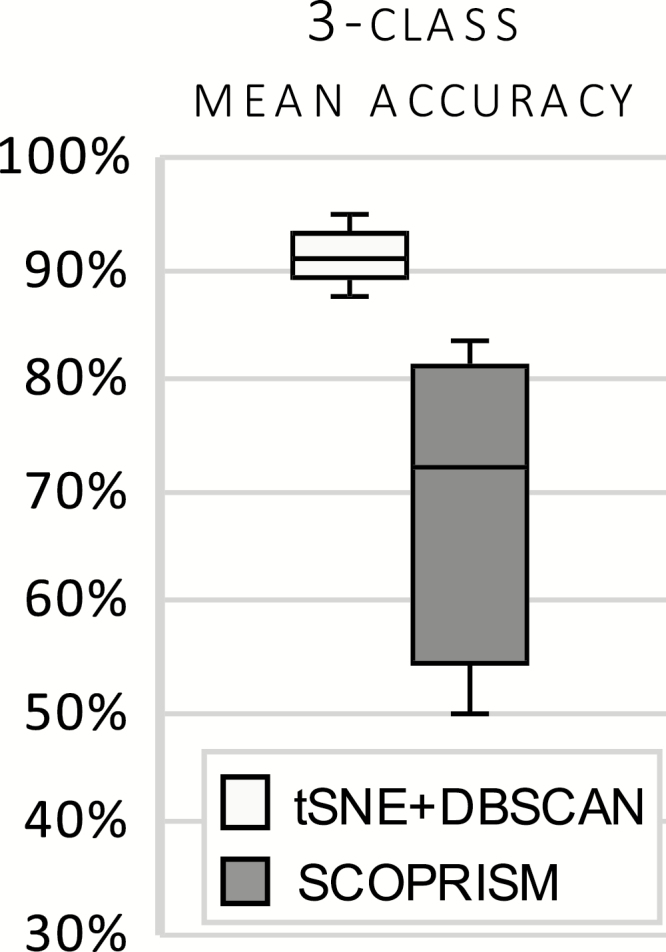
Mean accuracy of 3-class unsupervised classifiers for narcoleptic mice, n = 7. t-SNE+DBSCAN is the proposed unsupervised approach and is benchmarked against SCOPRISM.

Performance across states

The gross performance (mean accuracy) and performance by state of the two proposed classifiers and their respective benchmarks is shown in Figure 7. It should be noted that the CSL was applied to the output of each classifier to achieve a four-class accuracy. As shown, the CNN classifier exhibits superior performance compared to the SVM and the unsupervised methods.

Figure 7.

Gross and class-specific accuracy for each test dataset for narcoleptic mice, n = 7. Each classifier is trained on Day 1; results shown are from test sets Day 2 and compared against manual scores. Overall, the CNN performed best across states. Circle represents a statistical outlier.

Algorithm performance with respect to cataplexy

Cataplexy is the rarest label, with an approximate mean prevalence of 2%, which can obscure the algorithms’ performance for this specific state. As such, we performed further analysis for cataplexy using the methods described in Sensitivity/Specificity/Precision/F1-Score Section. Performance metrics with respect to cataplexy labels for narcoleptic mice across all classifiers are illustrated in Figure 8.

Figure 8.

Performance metrics for cataplexy with respect to each classfier. Each classifier is trained on Day 1; results shown are from test sets of Day 2 and compared against manual scores, n = 7. Circles represent statistical outliers.

Algorithm performance on wild-type mice

To address the algorithm performance on non-narcoleptic mice, we employed the proposed framework on datasets from wild-type mice. For each wild-type mouse, datasets D1 were used for training of the classifier and datasets D2 for testing (i.e. algorithms were trained on wild-type data). Accuracy across vigilance states and number of false-positive results are shown in Figure 9. All methods exhibit similar performance as with the narcoleptic mice, with the CNN yielding the lowest number of cataplexy false-positive labels per 24 h recording.

Figure 9.

Gross and class-specific accuracy of each classifier for wild-type mice, n = 7. Each classifier is trained on Day 1; results shown are from test sets Day 2 and compared against manual scores, n = 7. Cataplexy false positives represent the percent of incorrectly defined 10-s epochs over a 24-h recording.

Discussion

We presented two methods (along with their respective bases of comparison) for the scoring of vigilance states from EEG/EMG data. Scoring of wakefulness, non-REM sleep and REM sleep is performed by either a supervised classification or unsupervised clustering, whereas scoring of cataplexy is implemented by a post-processing layer.

Our supervised approach is based on a CNN architecture that takes raw time series data (down sampled to 100 Hz) and outputs labels and probability distributions (match percentages) for each state. Although the CNN requires previously scored data for training, it produces the most accurate labels (mean of 95%) when applied on test data compared to the other methods. Performance is optimal when a separate classifier is trained for each animal subject. As shown in CNN Classifier Generalization Across Animals Section, a single supervised classifier can be trained on data originating from several different animal subjects, and performs well on familiar-animal data; however, its performance on novel-animal data depends on the inter-subject variability and seems to be generally lower than the unsupervised approach. Thus, deploying a supervised classifier outside the animal (or group of animals) on which it was trained is not advisable. No matter how standardized the implantation procedure is, there are always differences in the obtained signal, which may be substantial enough to deteriorate the performance of a classifier which has not been trained on that animal (e.g. ATA287 in Table 1). Signal quality and variability between animals is an issue also encountered in human scoring, a fact which our human scorers had to deal with in our datasets as well. Potentially, greatly increasing the number of subjects (to the order of hundreds or thousands) available for the training of a single classifier would provide enough “diversity” in the data profiles for the network to be made robust to such variability. However, this is one of the caveats in dealing with the small number of subjects which may be studied at any given time in an animal sleep lab. This pronounced inter-subject variability within cohorts that lead to poor generalization across animals was also the reason why we did not investigate cross-cohort generalization. Variability in performance across different datasets/subjects is actually a common issue within machine learning in general, and an open area of research (transfer learning) [26].

The main advantages of the CNN are its high accuracy and ease of implementation, as well as the ability of a trained classifier to be deployed online for real-time scoring during the data acquisition process. Another advantage is the presence of the probability distribution over states, which not only offers a measure of classifier confidence, but also can be informative on the pathophysiology of cataplexy. Indeed, as shown in Figure 10, cataplexy is characterized by either a clear, sharp transition from W to R, or by a temporary mixture of states; this mixture of states during cataplectic events has also been reported using a similar computational approach in human narcolepsy patients [27].

Figure 10.

Examples of CNN detection of cataplexy (a-d), compared to a normal sleep bout (e). Colors blue, red, green, and teal correspond to W, N, R, and C, respectively. Cataplexy is characterized by either a clear, sharp transition from W to R (c), or by a temporary “mixing of states”, followed by R (a,b,d). HL: human expert label; PL: predicted label; Conf: prediction confidence.

Our unsupervised approach (tSNE+DBSCAN) transforms the EEG time series to the frequency domain (1–50 Hz range in 1 Hz resolution) and calculates of the variance of the EMG signal for each 10 s segment. The resulting 50-dimensional feature vectors are then mapped to a 2-dimensional population via t-SNE, and DBSCAN is employed for subsequent clustering. The main advantages of using tSNE+DBSCAN are that it does not require any prior knowledge on all or part of the data, such as human expert-labeling, and that it can be deployed individually for each dataset without assigning separate portions of it for training. Notably, our application of the unsupervised approach failed to identify a separate cluster for cataplexy, suggesting that the electrophysiology of cataplexy is insufficiently distinct from REM. Indeed, as illustrated in Figure 11, samples scored by human experts as cataplexy seem to typically overlap with those scored as REM sleep. This implies that if the temporal ordering of samples is ignored (in particular, the transitions between W, N, and R), the difference (if any) in frequency content between cataplexy and REM sleep samples must be rather subtle, thus overshadowed by the differences between the rest of the behavioral states. This observation is consistent with a clinical understanding of cataplexy, which defines it by the subjective experience of the patient (i.e. a symptom) rather than by electrophysiological criteria alone, and makes it challenging to study in a clinical sleep laboratory.

Figure 11.

Example trace of CNN classifier’s ability to accurately score cataplexy without the use of video. Colors blue, red, green, and teal correspond to W, N, R, and C, respectively. HL_A: Labels scored by a human expert using only EEG/EMG are scored as a normal sleep transition from non-REM to REM. With the addition of video, however, the EEG/EMG is scored as cataplexy due to clear behavioral arrest (HL_B, human label using a combination of EEG/EMG/Video). The CNN identifies the entire episode as cataplexy with some uncertainty in only the first two epochs (PL, predicted label by CNN). In this example, the algorithm is superior at detecting REM sleep than an expert scorer.

The advantages of the unsupervised method come at the cost of reduced accuracy (an average of 91%), and the inability to be deployed as an online (real time) scoring tool in the algorithm’s current form. Additionally, there is some increased complexity of use compared to the supervised approach, as the values of clustering parameters for DBSCAN are especially sensitive to the quality of the EEG/EMG signal and may require hand-tuning. The quality of the EEG signal in particular is critical for good performance and may explain why the herein reported performance values of SCOPRISM are so different from the ones reported in the original paper.

Another general issue with this method is the interpretation of clusters. If there is an electrophysiological artifact or natural process exhibited over a large number of samples which has an intensity that overshadows electrophysiological differences between behavioral states, a distinct cluster will form that is not necessarily attributable to a behavioral state. Thus, caution needs to be taken in the interpretation of clusters.

We note that we scored both the narcoleptic and the wild-type cohort separately and with both approaches. We used the supervised and unsupervised approach independently of each other in order to be able to evaluate the accuracy of each approach separately. While, in the absence of labels obtained from a human scorer, one could first obtain labels using the unsupervised approach and then employ the supervised approach utilizing these obtained labels, such an employment of the two methods in series would “entangle” the performance of both approaches without giving a clear picture of their individual accuracies, which we sought to provide here.

With respect to the performance metrics of the post-processing CSL, there is a clear advantage of the supervised learning approach compared to the unsupervised approach in the scoring of cataplexy, which can be attributed to the CNN’s superior ability to distinguish labels of REM sleep that are later converted to cataplexy labels by the CSL. Indeed, as seen in Figure 6(c) and (d), the unsupervised method faces some difficulty in separating between non-REM and REM sleep, tending to underestimate the REM label population. This, in turn, excludes many cases of cataplexy during the application of the CSL. This behavior explains why the unsupervised approach, combined with the CSL, typically tends to under-report cataplexy as seen in Figure 9. In contrast, the supervised approach has a much more robust performance across datasets, detecting virtually all cases of cataplexy which can be safely identified solely by means of EEG/EMG. Almost all cases of misclassification of cataplexy in the supervised approach were cases in which the algorithm reported non-REM sleep; however, upon inspection of those particular signal segments of the EEG/EMG, experts agreed that the signals indeed displayed all characteristics of non-REM sleep, and it was only the animal behavior as seen in the video recording that prompted the assignment of a cataplexy label (Figure 12). Thus, there are cases of cataplexy, at least as labeled by some experts, in which the EEG/EMG alone are insufficient to determine the label (Figure 12). Nevertheless, there were also cases in which the algorithm was able to pick up subtle abnormalities in the EEG/EMG that were not visible to the human scorer, and lead to the scoring of cataplexy based only on electrophysiology, despite the scorer having to rely on video (Figure 11). Despite the shortcomings due to the lack of video source information in the automated scoring of cataplexy, the CSL nevertheless displays very high specificity values, indicating that it is capable of detecting a very rare label with very few false positives. Anecdotally, another benefit of the algorithm was that it identified some episodes of cataplexy that were missed by the expert during the initial review.

Figure 12.

Example trace of cataplexy identified only by use of video. Colors blue, red, green, and teal correspond to W, N, R, and C, respectively. HL_A: Labels scored by a human expert using only EEG/EMG are scored as Non-REM to REM. HL_B: Labels scored by a human expert using EEG/EMG/Video are scored as cataplexy due to behavior. PL: Predicted label scored by CNN as non-REM sleep with some uncertainty throughout the episode.

All algorithms were tested on wild-type mice data to validate the CSL specificity. Cataplexy false positives are associated with misclassifications of REM sleep by each classifier, that are then modified into cataplexy labels by the CSL. Both proposed methods (CNN and t-SNE+DBSCAN) yielded a very low false-positive rate, less than 0.2%. Furthermore, the performance of all methods in classifying each behavioral state was consistent with the performance exhibited on narcoleptic data, with the CNN achieving the best performance. This demonstrates that the proposed methods can also be deployed in the scoring of wild-type mice.

With either approach presented, results may be manually corrected by experts as needed. Future efforts toward behavioral state scoring based upon animal and human electrophysiological data may be greatly facilitated and expedited by supervised and unsupervised machine learning. All algorithms implemented in this work (including example datasets) can be made available upon request.

Funding

This work has been supported by a Sleep Research Society Foundation Career Development Award to JTW, an Emory University Research Committee Award to JTW, a Pilot Translational and Clinical Studies Program Award of the Georgia Clinical & Translational Science Alliance to JTW, NIH NINDS grant K0NS8105929 to NPP, and a BRAIN Initiative UG3/UH3 to REG, grant 1UG3NS100559-01.

Conflict of interest statement: none declared.

References

- 1. Anaclet C, et al. Orexin/hypocretin and histamine: distinct roles in the control of wakefulness demonstrated using knock-out mouse models. J Neurosci. 2009;29(46):14423–14438. [DOI] [PMC free article] [PubMed] [Google Scholar]
- 2. Diniz Behn CG, et al. Abnormal sleep/wake dynamics in orexin knockout mice. Sleep. 2010;33(3):297–306. [DOI] [PMC free article] [PubMed] [Google Scholar]
- 3. Fujiki N, et al. Specificity of direct transition from wake to REM sleep in orexin/ataxin-3 transgenic narcoleptic mice. Exp Neurol. 2009;217(1):46–54. [DOI] [PMC free article] [PubMed] [Google Scholar]
- 4. Hara J, et al. Genetic ablation of orexin neurons in mice results in narcolepsy, hypophagia, and obesity. Neuron. 2001;30(2):345–354. [DOI] [PubMed] [Google Scholar]
- 5. Willie JT, et al. Distinct narcolepsy syndromes in Orexin receptor-2 and Orexin null mice: molecular genetic dissection of non-REM and REM sleep regulatory processes. Neuron. 2003;38(5):715–730. [DOI] [PubMed] [Google Scholar]
- 6. Libourel PA, et al. Unsupervised online classifier in sleep scoring for sleep deprivation studies. Sleep. 2015;38(5):815–828. [DOI] [PMC free article] [PubMed] [Google Scholar]
- 7. Kreuzer M, et al. Sleep scoring made easy-semi-automated sleep analysis software and manual rescoring tools for basic sleep research in mice. MethodsX. 2015;2:232–240. [DOI] [PMC free article] [PubMed] [Google Scholar]
- 8. Sunagawa GA, et al. FASTER: an unsupervised fully automated sleep staging method for mice. Genes Cells. 2013;18(6):502–518. [DOI] [PMC free article] [PubMed] [Google Scholar]
- 9. Brankack J, et al. EEG gamma frequency and sleep-wake scoring in mice: comparing two types of supervised classifiers. Brain Res. 2010;1322:59–71. [DOI] [PubMed] [Google Scholar]
- 10. Rytkönen KM, et al. Automated sleep scoring in rats and mice using the naive Bayes classifier. J Neurosci Methods. 2011;202(1):60–64. [DOI] [PubMed] [Google Scholar]
- 11. Gao V, et al. Multiple classifier systems for automatic sleep scoring in mice. J Neurosci Methods. 2016;264:33–39. [DOI] [PMC free article] [PubMed] [Google Scholar]
- 12. Goodfellow I, et al. Deep Learning. Cambridge, MA: MIT Press; 2016. [Google Scholar]
- 13. Ghassemi MM, et al. You Snooze, You Win: the PhysioNet/Computing in Cardiology Challenge. 2018. [DOI] [PMC free article] [PubMed] [Google Scholar]
- 14. Van Der Maaten L, Hinton G. Visualizing Data Using T-SNE. Vol 9; 2008. http://www.jmlr.org/papers/volume9/vandermaaten08a/vandermaaten08a.pdf. Accessed June 5, 2019. [Google Scholar]
- 15. Bastianini S, et al. SCOPRISM: a new algorithm for automatic sleep scoring in mice. J Neurosci Methods. 2014;235:277–284. [DOI] [PubMed] [Google Scholar]
- 16. Murphy KP. Machine Learning: A Probablistic Perspective. Cambridge, MA: The MIT Press; 2012. https://dl.acm.org/citation.cfm?id=2380985. Accessed July 10, 2019. [Google Scholar]
- 17. Scammell TE, et al. ; International Working Group on Rodent Models of Narcolepsy A consensus definition of cataplexy in mouse models of narcolepsy. Sleep. 2009;32(1):111–116. [PMC free article] [PubMed] [Google Scholar]
- 18. Ioffe S, et al. Batch normalization: accelerating deep network training by reducing internal covariate shift. Proc Int Conf Learn Represent. 2015;37:448–456 http://proceedings.mlr.press/v37/ioffe15.pdf. Accessed June 5, 2019. [Google Scholar]
- 19. Srivastava N, et al. Dropout: a simple way to prevent neural networks from overfitting. J Mach Learn Res. 2014;15(1):1929–1958. [Google Scholar]
- 20. Kingma DP, Lei Ba J. Adam: a method for stochastic optimization. In: Proceedings of the International Conference on Learning Representations (ICLR).; 2015. https://arxiv.org/pdf/1412.6980.pdf. Accessed June 5, 2019.
- 21. Chollet F, others. Keras. 2015. [Google Scholar]
- 22. Abadi M, et al. TensorFlow: Large-Scale Machine Learning on Heterogeneous Distributed Systems. www.tensorflow.org. Accessed June 5, 2019.
- 23. Mitra P, others. Chronux. [Google Scholar]
- 24. Ester M, et al. A density-based algorithm for discovering clusters in large spatial databases with noise. In: Proceedings of the Conference on Knowledge Discovery and Data Mining (KDD); 1996:226–231.
- 25. Pedregosa F, et al. Scikit-learn: machine learning in python. J Mach Learn Res. 2011;12:2825–2830. [Google Scholar]
- 26. Pan SJ, et al. A survey on transfer learning. IEEE Trans Knowl Data Eng. 2010;22(10):1345–1359. [Google Scholar]
- 27. Stephansen JB, et al. Neural network analysis of sleep stages enables efficient diagnosis of narcolepsy. Nat Commun. 2018;9(1):5229. [DOI] [PMC free article] [PubMed] [Google Scholar]