Backbone reconstruction in temporal networks from epidemic data

Abstract

Many complex systems are characterized by time-varying patterns of interactions. These interactions comprise strong ties, driven by dyadic relationships, and weak ties, based on node-specific attributes. The interplay between strong and weak ties plays an important role on dynamical processes that could unfold on complex systems. However, seldom do we have access to precise information about the time-varying topology of interaction patterns. A particularly elusive question is to distinguish strong from weak ties, on the basis of the sole node dynamics. Building upon analytical results, we propose a statistically-principled algorithm to reconstruct the backbone of strong ties from data of a spreading process, consisting of the time series of individuals' states. Our method is numerically validated over a range of synthetic datasets, encapsulating salient features of real-world systems. Motivated by compelling evidence, we propose the integration of our algorithm in a targeted immunization strategy that prioritizes influential nodes in the inferred backbone. Through Monte Carlo simulations on synthetic networks and a real-world case study, we demonstrate the viability of our approach.

I. INTRODUCTION

In the past few decades, network science has experienced significant developments, providing researchers with an array of powerful tools to represent and analyze complex biological, social, and technological systems [1]. Besides improving our knowledge on the very structure of complex systems, network science has contributed new paradigms to study dynamical processes unfolding on a complex system. These paradigms have shed light on the intertwining between structure and dynamics in the spread of epidemic diseases [2], diffusion of innovation [3], and opinion formation [4].

Empirical studies suggest that patterns of interactions between nodes in many complex networks evolve ceaselessly in time [5,6]. These interactions can be categorized into two main classes [7]. One class corresponds to interactions that are recurrently formed between node pairs, following dyadic relationships that are called strong ties [8]. Interactions in the workplace or family ties belong to this class, which forms the backbone of the network [9,10]. The second class encompasses interactions that are based on features of the nodes, which are not attributable to dyadic ties with other nodes. For instance, interactions among people queuing in a line or sitting on a plane belong to this class, whereby interactions are triggered by individual attributes such as extroversion in talking to strangers. These relationships are called weak ties [8]. Strong and weak ties concur in shaping the dynamic behavior of complex networks [11–13].

Activity driven networks (ADNs) have emerged as a valuable framework for temporal networks [14], allowing for modeling the coevolution of the network structure and the unfolding nodal dynamics at comparable timescales. The temporal nature of the network is captured through a single parameter that measures the node propensity to generate interactions. The distribution of this parameter, called activity, can be inferred from real-world data [14]. The potential of ADNs has been demonstrated through the study of several network problems, including epidemics [15–19], diffusion of innovation [20], opinion formation [21], and percolation [22].

In their fundamental incarnation, ADNs are an ideal tool to model weak ties, whereby the whole process of network assembly is driven by a node-specific attribute, the activity. Routed ADNs (RADNs) have been recently proposed to include strong ties within the ADN paradigm [23,24]. In this model, temporal connections are wired according to a stochastic rule that encapsulates both the topological information of strong ties and the unstructured connections of weak ties. RADNs share similarities with other approaches to include strong ties in ADNs, such as the superimposition of a static network [25,26], and the inclusion of memory mechanisms in the link wiring process [27,28].

The use of RADNs in real-world scenarios rely on accurate knowledge of the activity distribution and the topology of the backbone. While activities can be estimated following the literature on ADNs [14,29], the inference of the backbone of strong ties remains an open challenge. Preliminary efforts in this direction can be found in Ref. [30]. Therein, the authors have proposed a method to reconstruct the backbone of a temporal network from the direct observation of the pattern of interactions over an accessible time-window. Particularly elusive is the problem of distinguishing strong from weak ties from observations of node dynamics, which is typically the only knowledge available in real epidemiological settings [31].

In the technical literature, the problem of link reconstruction and prediction has been studied from a variety of angles, mostly relying on the direct observations of contacts [32–34]. Dealing with observations of nodal dynamics, several methods have been proposed to reconstruct patterns of interactions [35], including the use of similarity [36], information theory [37], belief propagation [38], likelihood maximization [39,40], compressed sensing [41,42], optimization [43], nonparametric Bayesian methods [44], and data-driven approaches [45,46]. However, these strategies are of limited use when strong and weak ties coexist, thereby presently challenging the inference of backbone networks from observations of node dynamics.

Drawing inspiration from Refs. [47,48], here we design a backbone detection algorithm that identifies strong ties from node dynamics, in the form of empirical data about a spreading process. Because of its widespread use in the study of epidemic outbreaks, we adopt the epidemiological lexicon throughout the paper when referring to the spreading dynamics. However, the application of our algorithm should not be considered limited to the epidemiological field, since spreading processes in temporal networks are widely used to model other phenomena, including diffusion of innovation in social groups [20] and information flow in brain networks [49–51].

Our algorithm is based on the intuition that strong ties should leave a distinguishable footprint on the temporal evolution of an epidemic outbreak. We analytically characterize such a footprint in terms of the probability for a node to contract the disease, given knowledge about the health state of other nodes. Building upon this analytical result, we formulate a statistically-principled algorithm to reconstruct the backbone topology. An extensive performance analysis is carried out by means of numerical simulations to demonstrate the effectiveness of the algorithm and identify potential limitations. Finally, we demonstrate the possibility of implementing the algorithm to inform immunization strategies that target influential nodes of the backbone. The effectiveness of the proposed technique is evaluated through Monte Carlo simulations both on synthetic networks and real-world data of face-to-face interactions in a high school [52].

II. MATHEMATICAL BACKGROUND

We provide mathematical details of the models herein used to study temporal networks with a backbone structure of strong ties, along with dynamical process.

A. Routed ADNs

We consider a network of $n$ nodes, each belonging to the node set $V=\{1,\cdots ,n\}$. Temporal undirected links are represented through time-varying adjacency matrix $A_t\in {\{0,1\}}^{n\times n}$, where $t\in {\mathbb{Z}}_{+}$ is the discrete time index. The adjacency matrix is assembled so that ${\left(A_t\right)}_{ij}=1$ if and only if node $i$ is connected with node $j$ at time $t$. We denote by $N_t^i$ the neighborhood of node $i$ at time $t$, that is, the set of other nodes to which $i$ is connected at time $t$.

Both strong and weak ties contribute to the evolution of $A_t$. Strong ties are described by an undirected and time-invariant adjacency matrix $G\in {\{0,1\}}^{n\times n}$. We indicate with $d_i$ the degree of node $i$ in the backbone network. Degrees are gathered in the degree vector $d\in {\mathbb{N}}^n$. Empirical evidence from real-world observations suggests that real-world backbones are often sparse [1] and nodes have bounded degree [53]. Without loss of generality, we assume that the backbone network does not contain isolated nodes, that is, $d_i\ge 1$, for all $i\in V$ [54].

Following Ref. [24], each node $i\in V$ is characterized by an activity parameter $a_i\in [0,1]$. At each time, node $i$ activates with probability $a_i$ and generates an undirected link with another node. The selection of which node to connect to is probabilistically dictated by a row-stochastic [55] matrix $P\in {\mathbb{R}}_{\ge 0}^{n\times n}$ such that

$$P=(1-\gamma )\frac{1}{n-1}J+\gamma \mathrm{diag}{\left(d\right)}^{-1}G,$$ (1)

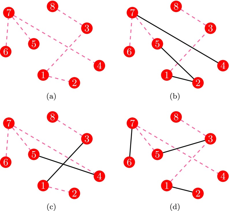
where $\gamma \in [0,1]$ is a constant parameter and $J$ is the $n\times n$ matrix of all ones, except the diagonal entries, which are set to 0. The generic entry $P_{ij}$ represents the probability that $i$ connects with $j$. The first term on the right hand side of Eq. (1) accounts for the weak ties, while the second summand models strong ties in the backbone. The parameter $\gamma \in [0,1]$ weights the role of strong versus weak ties in the formation of temporal links. When $\gamma =0$, the model reduces to a standard ADN [14], such that strong ties are uninfluential; when $\gamma =1$, the probability of a connection mirrors the adjacency matrix of the backbone network. A realization of an RADN is shown in Fig. 1.

FIG. 1.

Illustration of a backbone network (a) along with three consecutive realizations of an RADN (b–d) at time $t=0,1,2$, respectively. Red dashed links are the strong ties in the backbone, and black solid links are temporal links generated from nodes' activity.

To generate a temporal network from $t=0$, up to time $T$, we implement the following steps:

• (1)the temporal adjacency matrix is initialized as ${\left(A_t\right)}_{ij}=0$, for all $i,j\in V$;
• (2)each node $i\in V$ activates with probability $a_i$, independent of the others;
• (3)for each node $i$ that is active, a node $j$ is selected with probability $P_{ij}$, and we set ${\left(A_t\right)}_{ij}={\left(A_t\right)}_{ji}=1$; and
• (4)the time index $t$ is incremented by 1; if $t\ge T$, the algorithm is terminated, otherwise it is resumed to step 1.

B. Susceptible–infected–susceptible model

We focus on a susceptible–infected–susceptible (SIS) epidemic model [56]. In an SIS model, each node of the network is characterized by a binary health state. Specifically, at time $t$, node $i\in V$ is either susceptible to the disease ($X_t^i=0$) or infected ($X_t^i=1$). At each time, two contrasting mechanisms govern the evolution of the epidemic process: propagation and recovery. Each susceptible node can contract the disease through interactions with infected nodes.

The propagation of the disease may occur with probability $\lambda \in [0,1]$ along each link of the RADN independently of the others, such that

$$\mathbb{P}\left(X_{t+1}^i=1|X_t^i=0\right)=1-{(1-\lambda )}^{{\sum }_{j\in N_t^i}{X}_t^j}.$$ (2)

Following the recovery mechanism, instead, each node $i$ that is infected at time $t$, recovers at time $t+1$ with probability $\mu \in [0,1]$, becoming again susceptible to the epidemics. The generality of our theoretical approach suggests that our algorithm could be extended to more complex epidemic models on ADNs [29,57].

III. BACKBONE DETECTION ALGORITHM

We present here the main technical contribution of this work, which consists of an algorithm to detect the backbone of strong ties in a temporal network from epidemic data. Our method is based on the exact computation of the probability of a node to contract the disease given the health states of other nodes. Building on the knowledge about neighbors, we are able to pinpoint the effect of the presence of strong ties through a statistical test.

A. Conditional probabilities for RADNs

Given two nodes, $i$ and $j$, observed from the initial time 0 over a time-window of duration $T$, we define the following quantity:

$$\begin{array}{ccc}\hfill {\mathcal{P}}_{j\to i}& :=& {\displaystyle \frac{1}{T}\sum _{t=0}^{T-1}[\mathbb{P}\left(X_{t+1}^i=1|X_t^i=0,X_t^j=1\right)}\hfill \\ & & {\displaystyle -\mathbb{P}\left(X_{t+1}^i=1|X_t^i=0\right)].}\hfill \end{array}$$ (3)

The quantity ${\mathcal{P}}_{j\to i}$ summarizes the extent by which the infection of node $i$ over the time-window $0,\cdots ,T$ is explained by the disease propagation from node $j$ [58]. Intuition suggests that such a quantity is larger when $i$ and $j$ are connected by a strong tie, such that the infection of nodes connected by the backbone network will increase the chance of contracting the infection. For the considered RADN and a SIS process, mathematical analysis of this quantity, detailed in the Appendix, confirms this intuition.

Specifically, we demonstrate that, in the asymptotic limit of large time-windows, if there exists a strong tie between $i$ and $j$, that is, if $G_{ij}=1$, then

$$\begin{array}{ccc}\hfill {\displaystyle \underset{T\to \infty }{lim}{\mathcal{P}}_{j\to i}}& \ge & {\displaystyle \frac{\mu \lambda \gamma {\left[\left(1-\lambda \frac{a_i}{d_i}\right)\left(1-\lambda \frac{a_M}{d_m}\right)\right]}^{d_i-1}}{\lambda \left(a_i+\left(1-\gamma \left(1-\frac{d_i}{d_m}\right)\right)a_M\right)+\mu }\frac{1}{e^{\lambda (1-\gamma )(a_i+a_M)}}}\hfill \\ & & \times \left(\frac{a_i}{d_i}+\frac{a_j}{d_j}-\gamma \lambda \frac{a_i{a}_j}{d_i{d}_j}\right)>0,\hfill \end{array}$$ (4a)

almost surely, for any network size, where $a_M$ and $d_m$ are the maximum activity and the minimum backbone degree over the node set, respectively. However, if the two nodes are disconnected in the backbone, that is, if $G_{ij}=0$, then we find that in the asymptotic limit of large networks,

$$\underset{n\to \infty }{lim}{\mathcal{P}}_{j\to i}=0.$$ (4b)

As a consequence, if the size of the network is sufficiently large, the probability that a node becomes infected is not influenced by the health state of another, unless they share a strong tie. Based on this analytical result, we construct our identification algorithm, which starts from empirical observations of the disease dynamics to detect strong ties.

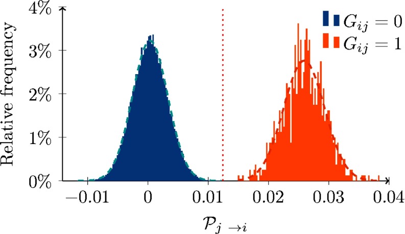
Figure 2 compares the empirical estimation of ${\mathcal{P}}_{j\to i}$ for pairs of nodes that share (orange) or not (blue) a strong tie. These simulations validate our analytical results and suggest that ${\mathcal{P}}_{j\to i}$ is close to its asymptotic expressions in Eq. (4), also for a reasonably small population size (that is, starting from $200–300$ nodes, according to our numerical simulations) and an observation window of limited duration. In fact, while the empirical distribution of the entries of ${\mathcal{P}}_{j\to i}$ that correspond to strong ties (in orange) is shifted and bounded away from 0, the empirical distribution of the entries that do not correspond to strong ties is centered at 0.

FIG. 2.

Empirical estimation of ${\mathcal{P}}_{j\to i}$ in a realization of an RADN with $n=200$ nodes, $\gamma =0.95, \lambda =0.9, \mu =0.1$, and $a_i=0.3$ for all nodes, over all the pairs of nodes $(i,j)\in V\times V$. The orange distribution relates to nodes that share a strong tie and the blue one to the opposite case. The backbone network is a 4-regular random graph. The network is simulated for $35000$ time steps. The figure suggests that conditioning on the state of node $j$ affects the infection probability for nodes that share a strong tie with $j$, confirming our analytical results. The red dotted line is the lower bound on ${\mathcal{P}}_{j\to i}$ in the presence of the strong tie $\{i,j\}$, computed using Eq. (4a).

By comparing our analytical bound from Eq. (4a) (dotted red line) with the empirical observation, we propose that our estimation, albeit conservative, yields an accurate estimate of the order of magnitude of ${\mathcal{P}}_{j\to i}$. The two empirical distributions are well separated and both of them can be accurately fitted by a Gaussian distribution (dashed blue and orange, respectively) with means equal to 0.000 and 0.026, respectively, and standard deviations both equal to 0.003. This evidence suggests that a central limit theorem should hold for ${\mathcal{P}}_{j\to i}$, which is defined as an average over $T$. As a consequence, we may conjecture that the length of the time-window $T$ plays a key role in shaping the two distributions and, consequently, in determining whether strong and weak ties are statistically distinguishable. More details to support our conjecture can be found in Sec. IV and in the Appendix.

B. Statistical test

Building on our analytical results, we put forward a statistically-principled analysis to determine the presence of a strong tie between the two nodes for a network of conveniently large size. To perform such an analysis, for any pair of nodes $i$ and $j$, we measure the following four quantities over the observation time-window of duration $T$:

• (a)the number of time steps in which node $i$ is susceptible, denoted as $s_i$;
• (b)the number of transitions of node $i$ from susceptible to infected, denoted as $i_i$;
• (c)the number of time steps in which node $i$ is susceptible and node $j$ is infected, denoted as $n_{ij}$; and
• (d)the number of transitions of node $i$ from susceptible to infected with node $j$ being infected at the previous time, denoted as $q_{ij}$.

From the first two quantities, we compute the ratio $r_i=i_i/s_i$, which measures the sampling probability that a susceptible node $i$ at time $t$ becomes infected at $t+1$.

According to Eq. (4b), if $i$ and $j$ do not share a strong tie, then the probability that $i$ contracts the infection should not be influenced by $j$, that is, $q_{ij}$ should be a realization of a Bernoulli trial with expected value equal to $r_i{n}_{ij}$. We set this as the null hypothesis of our statistical test, which is rejected if $q_{ij}$ is significantly larger than $r_i{n}_{ij}$. We associate with the node pair a $p$ value, coming from the binomial cumulative distribution, equal to

$${\pi }_{ij}=1-\sum _{h=0}^{q_{ij}-1}\left(\genfrac{}{}{0pt}{}{n_{ij}}{h}\right)r_i^h{\left(1-r_i\right)}^{n_{ij}-h}.$$ (5)

This procedure generates a set of $n-1$ statistical tests for each node, that is, $n(n-1)$ tests, overall. Hence, a multiple comparison correction should be implemented to assess whether each one of the null hypotheses can be rejected. We adopt the Benjamini–Hochberg procedure to control the false discovery rate, which offers a less conservative criterion with respect to the standard Bonferroni criterion [59]. This method is implemented as follows.

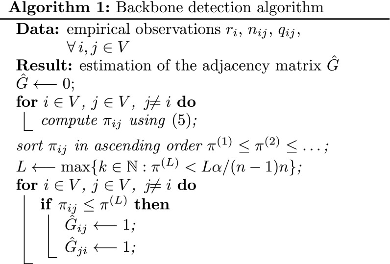
First, we set the level of significance $\alpha \in [0,1]$. The quantity $\alpha$ measures the largest admissible probability that at least one of the null hypotheses is erroneously rejected and it is typically set to a small quantity, to ensure the test significance. Then, the $n(n-1) p$ values are sorted in ascending order and denoted as ${\pi }^{\left(1\right)}<{\pi }^{\left(2\right)}<\cdots <{\pi }^{\left(\right(n-1\left)n\right)}$. Let $L$ be the largest integer for which it holds ${\pi }^{\left(L\right)}<L\alpha /(n-1)n$. Then, the null hypothesis is rejected for all the pairs of nodes associated with a $p$ value smaller than ${\pi }^{\left(L\right)}$. If the null exists hypothesis is rejected for $i$ and $j$, then we estimate that there exists a link in the backbone network between nodes $i$ and $j$. Hence, we set the corresponding element of the estimated backbone adjacency matrix $\widehat{G}$ as ${\widehat{G}}_{ij}={\widehat{G}}_{ji}=1$. We note that this is the step that requires the highest computational effort, since the $n(n-1) p$ values should be computed and sorted in ascending order. The algorithm can be implemented according to the pseudo code below.

Algorithm 1: Backbone detection algorithm

Examining more in depth the analytical results in Eq. (4a), we foresee some issues that might hinder the applicability of our algorithm, yielding a small value of ${\mathcal{P}}_{j\to i}$, even though a strong tie connecting $i$ to $j$ exists. In particular, this can occur in two cases. First, if both degrees $d_i$ and $d_j$ are large, such that the two nodes have a large degree centrality in the backbone network. Second, if both activities $a_i$ and $a_j$ are small. In the following, we present detailed numerical simulations with different parameter choices to demonstrate the accuracy of the algorithm.

IV. NUMERICAL VALIDATION

We validate our backbone detection algorithm on several synthetic datasets, to illustrate its applicability in real-world scenarios and identify potential limitations. These synthetic datasets consist of benchmark networks with $n=200$ nodes, generated according to the RADN paradigm described in Sec. II A. We consider different distributions for the nodes' activities and backbone degrees. Specifically, the latter follows a configuration model [1]. The epidemic process is simulated using the SIS model illustrated in Sec. II B with $\lambda =0.9$ and $\mu =0.1$. Unless otherwise specified, we set the significance level of the statistical test to $\alpha =0.05$ and the parameter $\gamma =0.95$.

A. Homogeneous activity distribution and homogeneous backbone

We first examine the possibility of identifying regular networks of strong ties against weak ties generated using a common activity value for the all nodes. In this scenario, the backbone is chosen to be a 4-regular random network and the activity is equal to $a_i=0.3$, for all $i\in V$.

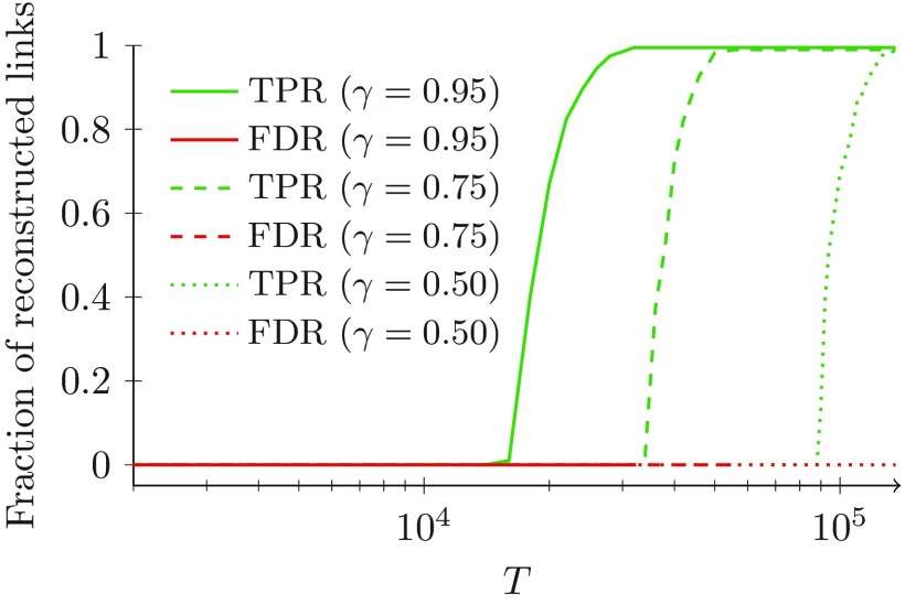
In Fig. 3, we plot the true positive rate (TPR), which is the fraction of links that the algorithm is able to correctly predict (green); and the false discovery rate (FDR), which is the ratio between the number of times it fails to properly identify a link and the number of links in the backbone (red). Perfect reconstruction is attained when the number of true positives is equal to the total number of positives ($\mathrm{TPR}=1$) and the number of false positives is equal to zero ($\mathrm{FDR}=0$). The computations are carried out for different values of $T$, such that larger values of $T$ imply access to a longer time-window for the estimation of the probabilities of transitions in the algorithm.

FIG. 3.

Fraction of strong ties identified by our algorithm in the scenario with both homogeneous activity distribution and backbone degrees, for different values of the parameter $\gamma$. The backbone is a 4-regular network with 200 nodes. The other parameters are $\lambda =0.9, \mu =0.1$, and $a_i=0.3$, for all the nodes.

For sufficiently large values of $T$, our algorithm is successful in exactly reconstructing the topology of the backbone, for any choice of the parameter $\gamma$. As suggested by the analytical expression in Eq. (4a), where $\gamma$ appears as a multiplicative coefficient, the smaller $\gamma$, the larger values of $T$ are required by our algorithm. Choosing small values of $T$ may hamper the correct identification of links, but it rarely results into the identification of false positives (for instance, only four false positives are overall identified for $\gamma =0.95$). Thus, increasing $T$, we progressively improve the detection of strong ties, attributing a very small quantity of wrong links to the backbone. This is an important feature of the algorithm, whereby all the links it discovers can be relied upon with an extremely high confidence. When few data is available, that is, for small $T$, the output of our algorithm could be poor. A possible strategy to circumvent the issue of limited data could be to not perform the multiple comparison correction, which, however, could beget a larger number of erroneous identifications.

B. Heterogeneous activity distribution and homogeneous backbone

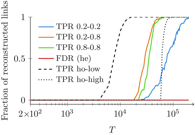
To better proxy a real-world setting, we release the assumption that all the nodes have the same activity. As a stepping stone, we consider the case in which nodes are randomly divided into two activity classes with 100 nodes each: low-activity nodes ($a_i=0.2$) and high-activity nodes ($a_i=0.8$). Similar to the previous analysis, the backbone is a 4-regular random network. To help teasing out the role of heterogeneity, we also simulate the scenarios in which all the nodes are either in the low- or high-activity classes.

Again, we examine the effect of $T$ on true and false positives, with respect to the number of positives. Results in Fig. 4 confirm those from Fig. 3, whereby the fraction of correctly identified links increases with $T$ and the fraction of misclassified links is always negligible. Comparing the three scenarios, we observe that large values of the activity have a negative effect on the performance of the algorithm. In fact, an increased observation window is required to detect strong ties in the homogeneous case with high activity, with respect to the scenario with low activity.

FIG. 4.

Fraction of strong ties correctly identified by our algorithm for both heterogeneous (“he”) and homogeneous (“ho”) activity distributions, and for homogeneous degree in the backbone. The backbone is a 4-regular network with $n=200$ nodes. The other parameters are $\gamma =0.95, \lambda =0.9$, and $\mu =0.1$. Three cases for the activity distribution are examined: all the nodes have the same activity $a_i=0.2$ (ho-low, dashed), $a_i=0.8$ (ho-high, dotted), and half the nodes have $a_i=0.2$ and half have $a_i=0.8$ (he, colored). For the last case of heterogeneous activities, the TPR curve is plotted with respect to links between nodes with low activity (blue), links between nodes of different activity (orange), and links between nodes with high activity (green). Only one FDR curve is plotted for all the cases, since they are practically indistinguishable (he, red).

Heterogeneity further reduces performance, hampering the detection of strong ties between low-activity nodes. Even though networks with a heterogeneous activity distribution require a longer window to correctly detect all the strong ties, we observe that, for sufficiently large $T$, our algorithm is able to correctly reconstruct the backbone, with a negligible fraction of erroneous identifications. Overall, these results are in agreement with the theoretical analysis in the Appendix, whereby decreasing the activities causes a reduction in the probability difference in Eq. (4a).

C. Homogeneous activity distribution and heterogeneous backbone

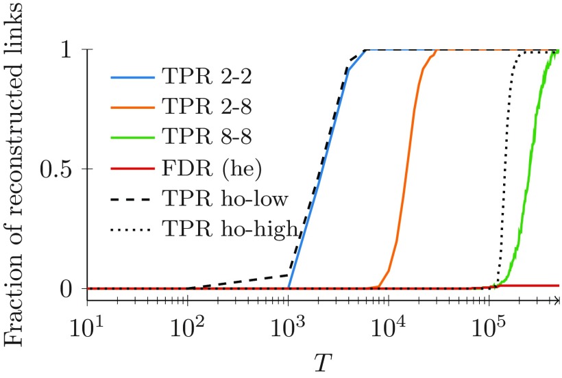
Next, we examine a backbone where the degree of the nodes is not held constant throughout the network. Specifically, we consider a network in which nodes are partitioned into two classes of 100 nodes each with low- ($d_i=2$) or high-degree ($d_i=8$). To avoid confounding, we maintain the activity at a common value of $a_i=0.3$, similar to results in Fig. 3. Once again, to facilitate the assessment of the effect of a heterogeneous degree distribution on the algorithm performance, we analyze two control cases in which all the nodes have the same low- or high-degree.

Figure 5 illustrates the fraction of links predicted as a function of $T$ for three considered settings. Consistently with our previous results, we observe that increasing the length of the observation steadily benefits the algorithm precision in inferring strong ties, as shown in Fig. 5. The number of false positives is always negligible, even for small values of $T$, confirming that the algorithm can be reliably utilized for backbone inference.

FIG. 5.

Fraction of strong ties correctly identified by our algorithm for both heterogeneous (“he”) and homogeneous (“ho”) backbones, and homogeneous activities $a_i=0.3$, for all the nodes. The other parameters are $n=200, \gamma =0.95, \lambda =0.9$, and $\mu =0.1$. Three cases for the backbone are examined: all the nodes have the same low-degree $d_i=2$ (ho-low, dashed); all the nodes have the same high-degree $d_i=8$ (ho-high, dotted); and half the nodes have $d_i=2$ and half have $d_i=8$ (he, colored). For the last case of heterogeneous degrees, the TPR curve is plotted with respect to links between nodes with low degree (blue), links between nodes of different degree (orange), and links between nodes with high degree (green). Only one FDR curve is plotted for all the cases, since they are practically indistinguishable (he, red).

Comparing the two homogeneous cases of low- and high-degree distributions, we register an expected decrease in performance when dealing with higher degrees. In this case, the value of added knowledge regarding the state of health of one node is diluted by the presence of many other neighbors that could have triggered the infection. Analytical results in the Appendix provide a theoretical basis for this explanation, whereby increasing the values of the degree causes a reduction in the probability difference in Eq. (4a).

As one might expect, the performance of the algorithm toward the inference of the heterogeneous network is in between the two cases of homogeneous networks. To gain further insight into the relationship between topological features and successful reconstruction, we can isolate the specific links that are first detected by the algorithm for small values of $T$. In agreement with our analytical result in Eq. (4a), the links that require shorter observations are incident to low-degree nodes. These links encompass both strong ties between low-degree nodes and strong ties between nodes with high and low degrees that might exemplify dissortative structures of real networks [60,61]. Longer time-windows are required for detecting links that connect pairs of high-degree nodes.

D. Highly heterogeneous activity distribution and backbone

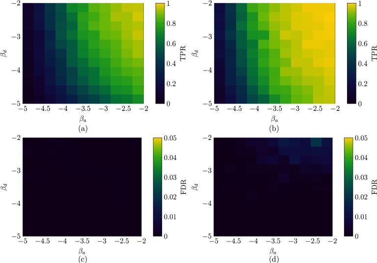
To offer insight on the performance of our algorithm over a wider class of RADNs, we systematically examine a two-dimensional grid of salient parameters. We assume that both the activity and the degree distributions follow a power-law with exponents ${\beta }_a$ and ${\beta }_d$, respectively. We vary each parameter from $-5$ to $-2$, which are representative of real-world scenarios [62]. Parameters are varied in 11 steps with cutoffs at 0.1 and 1 for the activity, and at 1 and $n-1$ for the degree.

We observe that smaller values of the exponent of a power-law yield distributions with a larger dispersion, in which most of the nodes have small activity (degree) and few have an extremely high activity (degree). Two different realizations are examined, one with $T=10000$ and $T=30000$, respectively. The weight $\gamma$ is reduced to 0.5 to guarantee the spread of the epidemic diseases for all the choices of parameters investigated and the network size is increased to $n=300$ to ensure the presence of high-degree (activity) nodes in the power-law distributions. The epidemic parameters are set as $\lambda =0.9$ and $\mu =0.1$, similar to the simulations in Sec. IV.

From Fig. 6, we recognize a marked effect of the parameters on the performance of our algorithm. For lower values of both parameters, ${\beta }_a$ and ${\beta }_d$, our algorithm fails to identify the backbone, under-predicting the number of strong ties. This is in agreement with Figs. 4 and 5, which indicate that longer observation windows are required to infer the backbone when the RADN is dominated by high-degree and high-activity nodes. The best performance is attained for higher values of the two parameters. In this case, the algorithm correctly detects all the strong ties, with a very small quantity of false positives.

FIG. 6.

TPR (a, b) and FDR (c, d) of our algorithm implemented on a network of $n=300$ nodes with heterogeneity in both activity distribution and backbone degree, for an observation window of $T=10000$ time steps (a, c) or $T=30000$ time steps (a, c). Both activities and backbone degrees follow power-law distributions with exponents ${\beta }_a$ and ${\beta }_d$, respectively. Other parameters are set to $\lambda =0.9, \mu =0.1$, and $\gamma =0.5$. Each point is an average of ten independent simulations.

Comparing the results for $T=10000$ and $T=30000$, interestingly, ${\beta }_a$ seems to have a stronger effect on performance than ${\beta }_d$, whereby at $T=30000$, the algorithm is able to detect most of the strong ties for small values of ${\beta }_d$ but its performance is strained when examining small values of ${\beta }_a$. This confirms our preliminary observation from Fig. 4 that heterogeneity in the activity distribution hampers the detection of strong ties.

V. APPLICATION TO TARGETED IMMUNIZATION

In epidemiology, knowledge about the backbone network might offer valuable information about how diseases spread and which is the role played by individuals [63]. In this vein, we conclude this paper by presenting an application of our algorithm to design a targeted immunization protocol. Our control strategy observes the disease spreading for a finite time-window to identify the backbone network, and then utilizes such an inference to prioritize immunization of nodes in the network according to a centrality criterion. Specifically, we immunize nodes according to decreasing values of their PageRank centrality [64]. By means of Monte Carlo numerical simulations, we evaluate the performance of the approach against a randomized immunization, where no information regarding the backbone is utilized.

Similar to the analysis in Sec. IV D, we examine a benchmark network with $n=300$ nodes. The backbone is generated using a configuration model with power-law degree distribution of power ${\beta }_d=-3$ and cutoffs at 1 and $n-1$. Activities are also drawn from a power-law distribution with exponent ${\beta }_a=-3$ and lower cutoff at 0.1. We consider an SIS epidemic with $\lambda =0.9$ and $\mu =0.1$. We run the model over a window of $50000$ time steps implementing our algorithm to identify the backbone. At this time, we execute two control strategies (targeted and randomized), with a number of interventions limited to $5\%$ of the total number of nodes. We perform Monte Carlo simulations by averaging over 100 independent runs of the two control strategies.

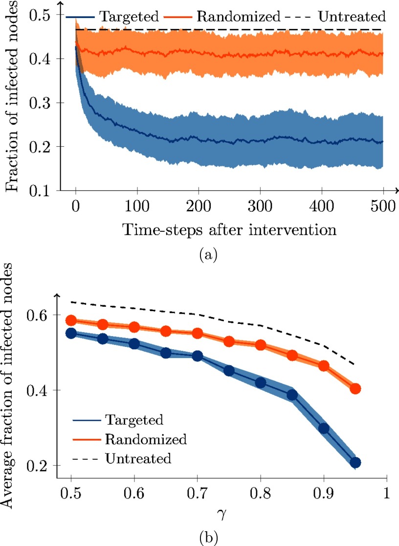
The results of these simulations are summarized in Fig. 7. In Fig. 7(a), we compare the performance of the two immunization strategies for $\gamma =0.95$, as in the numerical analysis in Sec. IV. While randomized immunization decreases the portion of infected nodes by $13\%$, targeted intervention decreases it by $55\%$, on average. The difference between these two strategies is statistically significant ($p\text{value}\ll 0.0001$, according to a two-sample $z$ test) comparing the average fraction of infected individuals after the implementation of the immunization strategy, for 100 independent runs. In Fig. 7(b), instead, the comparison between the two techniques is conducted for different values of the parameter $\gamma$, spanning from 0.5 to 0.95 in steps of 0.05. Therein, we report the average fraction of infected nodes in the 500 time steps that follow the application of the control strategy. Predictably, the larger the parameter $\gamma$, the stronger the improvement of the targeted immunization with respect to the randomized one. In fact, for small values of $\gamma$, the backbone has a marginal role on the link formation process, reducing the effect of targeted immunization exploiting the centrality measures in the backbone. However, the difference between the two strategies is statistically significant in all the performed simulations.

FIG. 7.

Monte Carlo estimation over 100 runs of the effect of randomized (orange) and targeted (blue) immunization on the fraction of infected nodes. Dotted lines indicate the fraction of infected nodes in the absence of any immunization technique. In (a), we show the entire realizations for $\gamma =0.95$. The solid line is the average, while the light band is one standard deviation. In (b), we compare the average fraction of infected nodes for different values of $\gamma$. Bands identify $95\%$ confidence intervals. Other parameters are $n=300, {\beta }_d={\beta }_a=-3, \lambda =0.9$, and $\mu =0.1$.

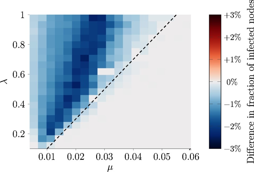
Encouraged by these promising results, we apply our targeted immunization technique to real-world face-to-face interactions measured through proximity sensors in a high school [52], available at Ref. [65]. The dataset comprises $188508$ temporal links, generated over $T=7375$ time steps among $n=327$ nodes. We run an SIS epidemic model for half of the available dataset, starting from a fraction of one third of infected nodes, selected uniformly at random. Then, $5\%$ of the nodes is immunized following either the randomized or the targeted strategy. By performing an extensive Monte Carlo simulation with $1000$ runs, we compare the two strategies for different values of the epidemic parameters $\lambda$ and $\mu$. Figure 8 demonstrates that our immunization technique should always be preferred to randomized immunization, whereby, for most parameter choices, it outperforms randomized immunization.

FIG. 8.

Difference in the fraction of infected nodes after the immunization phase, between the randomized and the targeted strategy (color coded) in the high-school case study [65]. The dashed line represents the epidemic threshold [56], below which none of the nodes is infected at the onset of the immunization strategy. Darker blue areas identify parameter regions where targeted immunization has superior outcome. Each point is an average of $1000$ independent simulations.

VI. CONCLUSIONS

In this work, we have proposed an algorithm to unveil the backbone of strong ties in a temporal network from empirical data of a spreading process unfolding on the network nodes. Building on analytical insight regarding the role of strong ties on the process, we have put forward a statistically-principled approach to discover strong ties from empirical data. Extensive simulations have been performed to assess the effectiveness of the proposed technique, which has proved to be reliable in a variety of scenarios. Finally, we have examined the integration of the proposed algorithm in the solution of an important challenge in epidemiology, namely, targeted immunization during an outbreak. The main contributions of this work are: (i) the analytical computation of the effect of strong ties on the infection probability for a susceptible–infected–susceptible epidemic model on routed activity driven networks; (ii) the design of a backbone detection algorithm and its numerical validation; and (iii) the implementation of a targeted immunization technique.

The promising preliminary results of our numerical analysis pave the way for several avenues of future research. We aim to rigorously assess the performance of our algorithm, as a function of the network size and the duration of the window of observation. Future efforts should focus on the development of accurate methods to deal with limited data, without increasing the number of erroneous identifications. In the analytical derivation of our bounds, we specialize the computations to the SIS epidemic model. However, the generality of our proving argument suggests that similar bounds could be established for other models, as well, provided that they do not admit permanently attractive states. These achievements would be key to provide a theoretical basis for the generalization of our algorithm to deal with other dynamics, including richer epidemic processes or opinion diffusion. Such an extension will be part of our future research. In most real-world scenarios, it is not tenable to have access to the entire node set, thereby calling for methods to discover missing nodes, beyond links.

The ability to reconstruct the structure of the backbone of a complex system from the observation of an unfolding spreading process finds application in disparate fields of investigation. Besides implementations to unveil the structure of social networks, one should mention the field of connectomics [66]. The goal of this area of research is to reconstruct connection patterns in animal and human brains, toward an improved understanding of the relationship between network structure and cognitive functionalities. We believe that our algorithm may be of help to connectomics by offering a pathway for the identification of recurrent interactions among the hubs of the brain network. Finally, our study on targeted immunization has demonstrated how information about the backbone can be leveraged to design effective control techniques that could steer the behavior of dynamical systems. Extending the framework to other disease models and mathematically proving performance bounds is the objective of future research.

APPENDIX: COMPUTATION OF THE CONDITIONAL PROBABILITIES

We compute the infection probability for node $i$ at time instant $t$, for either the case in which we include or exclude knowledge about node $j$. Let $x_1,\cdots ,x_n$ be the state of the system at time $t$, then the RADN model indicates that

$$\mathbb{P}\left(X_{t+1}^i=1|X_t^i=0\right)=1-\prod _{k\in V\setminus \left\{i\right\}}\left(1-\lambda a_i{P}_{ik}{x}_k\right)\left(1-\lambda a_k{P}_{ki}{x}_k\right).$$ (A1)

Upon conditioning on $X_t^j=1$, we factor the term associated with $j$ out of the multiplication to obtain

$${\displaystyle \mathbb{P}\left(X_{t+1}^i=1|X_t^i=0,X_t^j=1\right)=1-(1-\lambda a_i{P}_{ij})(1-\lambda a_j{P}_{ji})\prod _{k\in V\setminus \{i,j\}}(1-\lambda a_i{P}_{ik}{x}_k)(1-\lambda a_k{P}_{ki}{x}_k).}$$ (A2)

First, we consider the case in which nodes $i$ and $j$ do not share a strong tie, that is $G_{ij}=G_{ji}=0$. In this case, from Eq. (1) we derive $P_{ij}=P_{ji}=(1-\gamma )/(n-1)$. We substitute $P_{ij}$ and $P_{ji}$ in Eqs. (A1) and (A2), and we compute the limit for $n\to \infty$ of their difference as

$$\begin{array}{cc}& \underset{n\to \infty }{lim}\mathbb{P}\left(X_{t+1}^i=1|X_t^i=0,X_t^j=1\right)-\mathbb{P}\left(X_{t+1}^i=1|X_t^i=0\right)\hfill \\ & {\displaystyle =\underset{n\to \infty }{lim}\left[\left(1-\frac{\lambda (1-\gamma )a_i{x}_j}{n-1}\right)\left(1-\frac{\lambda (1-\gamma )a_j{x}_j}{n-1}\right)-\left(1-\frac{\lambda (1-\gamma )a_i}{n-1}\right)\left(1-\frac{\lambda (1-\gamma )a_j}{n-1}\right)\right]}\hfill \\ & {\displaystyle \times \prod _{k\in V\setminus \{i,j\}}(1-\lambda a_i{P}_{ik}{x}_k)(1-\lambda a_k{P}_{ki}{x}_k)}\hfill \\ & {\displaystyle =\underset{n\to \infty }{lim}\left[\frac{\lambda (1-\gamma )(a_i+a_j)(1-x_j)}{n-1}-\frac{{\lambda }^2{(1-\gamma )}^2{a}_i{a}_j(1-x_j)}{{(n-1)}^2}\right]\prod _{k\in V\setminus \{i,j\}}(1-\lambda a_i{P}_{ik}{x}_k)(1-\lambda a_k{P}_{ki}{x}_k)}\hfill \\ & {\displaystyle \le \underset{n\to \infty }{lim}\frac{\lambda (1-\gamma )(a_i+a_j)}{n-1}=0.}\hfill \end{array}$$ (A3)

We note that Eq. (A3) is the generic summand of ${\mathcal{P}}_{j\to i}$ in Eq. (3), from which the claim in Eq. (4b) follows. We further observe that each of the summands of ${\mathcal{P}}_{j\to i}$ is a nonnegative random variable, which is bounded from above by the estimation in Eq. (A3). Even though these random variables are not independent and not identically distributed (since they depend on the time-series of the nodes' health state that are self-correlated) they are bounded and their correlation tends to 0 in the long-time. Hence, a central limit theorem applies to ${\mathcal{P}}_{j\to i}$, according to Ref. [67]. Such an observation guarantees that ${\mathcal{P}}_{j\to i}$ converges to a Gaussian distribution, as supported by the numerics in Fig. 2. However, an explicit statement of the central limit theorem cannot be readily formulated, since it requires the computation of the variance.

We now consider the case in which nodes $i$ and $j$ share a strong tie, that is, $G_{ij}=G_{ji}=1$. Similar to the previous analysis, from Eq. (1) we derive $P_{ij}=(1-\gamma )/(n-1)+\gamma /d_i$ and $P_{ji}=(1-\gamma )/(n-1)+\gamma /d_j$. Defining the neighborhood of node $i$ in the backbone $N_G^i:=\{j\in V:G_{ij}=1\}$, we proceed specializing to the present case the difference between Eqs. (A1) and (A2) at time $t$. Considering that ${(1-k/x)}^{x-1}\ge 1/e^k$, for any $x\ge 1$ and $k>0$, and that $d_i\le n-1$, for any $i\in V$, we compute

$$\begin{array}{cc}& \mathbb{P}\left(X_{t+1}^i=1|X_t^i=0,X_t^j=1\right)-\mathbb{P}\left(X_{t+1}^i=1|X_t^i=0\right)\hfill \\ & {\displaystyle =\left\{\left[1-\lambda a_i{x}_j\left(\frac{\gamma }{d_i}+\frac{1-\gamma }{n-1}\right)\right]\left[1-\lambda a_j{x}_j\left(\frac{\gamma }{d_j}+\frac{1-\gamma }{n-1}\right)\right]-\left[1-\lambda a_i\left(\frac{\gamma }{d_i}+\frac{1-\gamma }{n-1}\right)\right]\left[1-\lambda a_j\left(\frac{\gamma }{d_j}+\frac{1-\gamma }{n-1}\right)\right]\right\}}\hfill \\ & {\displaystyle \times \prod _{k\in V\setminus \{i,j\}}(1-\lambda a_i{P}_{ik}{x}_k)(1-\lambda a_k{P}_{ki}{x}_k)}\hfill \\ & {\displaystyle \ge \lambda \gamma (1-x_j)\left(\frac{a_i}{d_i}+\frac{a_j}{d_j}-\lambda \gamma \frac{a_i{a}_j}{d_i{d}_j}\right)\prod _{k\in N_G^i\setminus \left\{j\right\}}(1-\lambda a_i{P}_{ik}{x}_k)(1-\lambda a_k{P}_{ki}{x}_k)\prod _{h\notin N_G^i\cup \left\{i\right\}}(1-\lambda a_i{P}_{ih}{x}_h)(1-\lambda a_h{P}_{hi}{x}_h)}\hfill \\ & {\displaystyle \ge \lambda \gamma (1-x_j)\left(\frac{a_i}{d_i}+\frac{a_j}{d_j}-\lambda \gamma \frac{a_i{a}_j}{d_i{d}_j}\right)\prod _{k\in N_G^i\setminus \left\{j\right\}}\left(1-\frac{\lambda a_i}{d_i}\right)\left(1-\frac{\lambda a_k}{d_k}\right)\prod _{h\notin N_G^i\cup \left\{i\right\}}\left(1-\frac{\lambda (1-\gamma )a_i}{n-1}\right)\left(1-\frac{\lambda (1-\gamma )a_k}{n-1}\right)}\hfill \\ & {\displaystyle \ge \lambda \gamma (1-x_j)\left(\frac{a_i}{d_i}+\frac{a_j}{d_j}-\lambda \gamma \frac{a_i{a}_j}{d_i{d}_j}\right){\left[\left(1-\frac{\lambda a_i}{d_i}\right)\left(1-\frac{\lambda a_M}{d_m}\right)\right]}^{d_i-1}{\left[\left(1-\frac{\lambda (1-\gamma )a_i}{n-1}\right)\left(1-\frac{\lambda (1-\gamma )a_M}{n-1}\right)\right]}^{n-1-d_i}}\hfill \\ & {\displaystyle \ge \frac{\lambda \gamma }{exp\left\{\lambda (1-\gamma )(a_i+a_M)\right\}}{\left(1-\lambda \frac{a_i}{d_i}\right)}^{d_i-1}{\left(1-\lambda \frac{a_M}{d_m}\right)}^{d_i-1}\left(\frac{a_i}{d_i}+\frac{a_j}{d_j}-\lambda \gamma \frac{a_i{a}_j}{d_i{d}_j}\right)(1-x_j)=:F\left(x_j\right),}\hfill \end{array}$$ (A4)

where $a_M$ is the maximum node activity and $d_m$ is the minimum degree in the backbone. The bounding function $F\left(x_j\right)$ is such that $F\left(1\right)=0$, and $F\left(0\right)>0$, for any $\gamma >0$.

We now focus on the variable $X_t^j$. According to the SIS dynamics described in Sec. II B, $X_t^j$ changes from 1 to 0 with probability equal to $\mu$, while the probability of switching from 0 to 1 depends on the health state of the other nodes, according to Eq. (A1). However, it can be bounded from above as follows:

$$\begin{array}{ccc}\hfill {\displaystyle \mathbb{P}\left(X_{t+1}^i=1|X_t^i=0\right)}& =& \mathbb{P}\left(\bigcup _{k\in V\setminus \left\{i\right\}}\left\{i\text{is}\text{infected}\text{by}k\right\}\right)\le \sum _{k\in V\setminus \left\{i\right\}}\mathbb{P}\left(\left\{i\text{is}\text{infected}\text{by}k\right\}\right)\hfill \\ & =& {\displaystyle \sum _{k\in V\setminus \left\{i\right\}}\lambda a_i{P}_{ik}{x}_k+\lambda a_k{P}_{ki}{x}_k-{\lambda }^2{a}_i{a}_k{P}_{ik}{P}_{ki}{x}_k\le \lambda \sum _{k\in V\setminus \left\{i\right\}}(a_i{P}_{ik}+a_M{P}_k)}\hfill \\ & =& \lambda \left\{a_i+\left[1-\gamma \left(1-\frac{d_i}{d_m}\right)\right]\right\}{a}_M.\hfill \end{array}$$ (A5)

Hence, the frequency of $X_t^j=0$ converges almost surely to at least $\mu /(\lambda (a_i+(1-\gamma (1-d_i/d_m))a_M)+\mu )$ for $T\to \infty$. Hence, using Eq. (A4) and the definition of ${\mathcal{P}}_{j\to i}$ in Eq. (3), the latter quantity can be bounded from below as follows:

$$\begin{array}{ccc}\hfill {\displaystyle \underset{T\to \infty }{lim}{\mathcal{P}}_{j\to i}}& =& {\displaystyle \underset{T\to \infty }{lim}\frac{1}{T}\sum _{t=0}^{T-1}\left[\mathbb{P}\left(X_{t+1}^i=1|X_t^i=0,X_t^j=1\right)-\mathbb{P}\left(X_{t+1}^i=1|X_t^i=0\right)\right]\ge \underset{T\to \infty }{lim}\frac{1}{T}\sum _{t=0}^{T-1}F\left(X_t^i\right)}\hfill \\ & =& {\displaystyle \underset{T\to \infty }{lim}\frac{1}{T}\sum _{t\in \{0,\cdots ,T-1\}:X_t^i=0}F\left(0\right)\ge \frac{\mu }{\lambda \left\{a_i+\left[1-\gamma \left(1-\frac{d_i}{d_m}\right)\right]a_M\right\}+\mu }F\left(0\right)}\hfill \\ & \ge & {\displaystyle \frac{\mu \lambda \gamma }{e^{\lambda (1-\gamma )(a_i+a_M)}(\lambda \{a_i+[1-\gamma (1-d_i/d_m)]a_M\}+\mu )}{\left(1-\lambda \frac{a_i}{d_i}\right)}^{d_i-1}{\left(1-\lambda \frac{a_M}{d_m}\right)}^{d_i-1}\left(\frac{a_i}{d_i}+\frac{a_j}{d_j}-\gamma \lambda \frac{a_i{a}_j}{d_i{d}_j}\right)}>0.\hfill \end{array}$$ (A6)

As shown in Fig. 2, our bound is accurate, albeit conservative. The main bottlenecks for improving the bound are in the substitution of the random variables $X_t^j$ with 1 in Eq. (A4) and in the estimation of the time elapsed with $X_t^j=0$ in the derivation of Eq. (A6). To obtain a tighter bound, one should rigorously compute the endemic state of an SIS model over an RADN, which is a nontrivial open problem [17].

Similar to our observations following Eq. (A3), we should note that a central limit theorem could in principle be established here as well, since ${\mathcal{P}}_{j\to i}$ is a temporal average of the transition probabilities. However, the derivation of its explicit statement is not possible, since it requires the exact computation of mean and variance of the summands.

We conclude the Appendix by commenting that our derivation is performed by using specific properties of the SIS epidemic model. We believe that a similar argument could be pursued to establish rigorous bounds on the transition probabilities for other dynamics, including more complex and realistic epidemics processes, or opinion dynamics, such as the voter model. In fact, the key properties of our argument is that the state transitions (from susceptible to infected) are triggered by the interactions and that they occur multiple times, due to the spontaneous recovery process. The former leaves the footprint of strong ties on the nodal dynamics, the latter affords the use of statistical tests to ensure significance to our results.

REFERENCES

- [1].M. E. Newman, SIAM Rev. 45, 167 (2003). 10.1137/S003614450342480 [DOI] [Google Scholar]
- [2].R. Pastor-Satorras, C. Castellano, P. Van Mieghem, and A. Vespignani, Rev. Mod. Phys. 87, 925 (2015). 10.1103/RevModPhys.87.925 [DOI] [Google Scholar]
- [3].A. Montanari and A. Saberi, Proc. Natl. Acad. Sci. USA 107, 20196 (2010). 10.1073/pnas.1004098107 [DOI] [PMC free article] [PubMed] [Google Scholar]
- [4].P.-P. Li, D.-F. Zheng, and P. M. Hui, Phys. Rev. E 73, 056128 (2006). 10.1103/PhysRevE.73.056128 [DOI] [PubMed] [Google Scholar]
- [5].P. Holme and J. Saramäki, Phys. Rep. 519, 97 (2012). 10.1016/j.physrep.2012.03.001 [DOI] [Google Scholar]
- [6].P. Holme, Eur. Phys. J. B 88, 234 (2015). 10.1140/epjb/e2015-60657-4 [DOI] [Google Scholar]
- [7].M. S. Granovetter, Am. J. Sociol. 78, 1360 (1973). 10.1086/225469 [DOI] [Google Scholar]
- [8].N. E. Friedkin, Soc. Netw. 3, 273 (1982). 10.1016/0378-8733(82)90003-X [DOI] [Google Scholar]
- [9].V. Gemmetto, A. Cardillo, and D. Garlaschelli, arXiv:1706.00230.
- [10].J.-P. Onnela, J. Saramäki, J. Hyvönen, G. Szabó, D. Lazer, K. Kaski, J. Kertész, and A.-L. Barabási, Proc. Natl. Acad. Sci. USA 104, 7332 (2007). 10.1073/pnas.0610245104 [DOI] [PMC free article] [PubMed] [Google Scholar]
- [11].P. Shu, M. Tang, K. Gong, and Y. Liu, Chaos 22, 043124 (2012). 10.1063/1.4767955 [DOI] [PMC free article] [PubMed] [Google Scholar]
- [12].M. Karsai, N. Perra, and A. Vespignani, Sci. Rep. 4, 4001 (2014). 10.1038/srep04001 [DOI] [PMC free article] [PubMed] [Google Scholar]
- [13].K. Sun, A. Baronchelli, and N. Perra, Eur. Phys. J. B 88, 326 (2015). 10.1140/epjb/e2015-60568-4 [DOI] [Google Scholar]
- [14].N. Perra, B. Gonçalves, R. Pastor-Satorras, and A. Vespignani, Sci. Rep. 2, 1 (2012). 10.1038/srep00469 [DOI] [PMC free article] [PubMed] [Google Scholar]
- [15].S. Liu, N. Perra, M. Karsai, and A. Vespignani, Phys. Rev. Lett. 112, 040601 (2014). 10.1103/PhysRevLett.112.040601 [DOI] [PubMed] [Google Scholar]
- [16].A. Rizzo, M. Frasca, and M. Porfiri, Phys. Rev. E 90, 042801 (2014). 10.1103/PhysRevE.90.042801 [DOI] [PubMed] [Google Scholar]
- [17].L. Zino, A. Rizzo, and M. Porfiri, Phys. Rev. Lett. 117, 228302 (2016). 10.1103/PhysRevLett.117.228302 [DOI] [PubMed] [Google Scholar]
- [18].G. Petri and A. Barrat, Phys. Rev. Lett. 121, 228301 (2018). 10.1103/PhysRevLett.121.228301 [DOI] [PubMed] [Google Scholar]
- [19].L. Zino, A. Rizzo, and M. Porfiri, SIAM J. Appl. Dyn. Syst. 17, 2830 (2018). 10.1137/18M1171485 [DOI] [Google Scholar]
- [20].A. Rizzo and M. Porfiri, Eur. Phys. J. B 89, 20 (2016). 10.1140/epjb/e2015-60933-3 [DOI] [Google Scholar]
- [21].D. Li, D. Han, J. Ma, M. Sun, L. Tian, T. Khouw, and H. E. Stanley, Europhys. Lett. 120, 28002 (2017). 10.1209/0295-5075/120/28002 [DOI] [Google Scholar]
- [22].M. Starnini and R. Pastor-Satorras, Phys. Rev. E 89, 032807 (2014). 10.1103/PhysRevE.89.032807 [DOI] [PubMed] [Google Scholar]
- [23].C. Bongiorno, L. Zino, and A. Rizzo, in Proceedings of the 57th IEEE Conference on Decision and Control (IEEE, Miami Beach, Florida USA, 2018), pp. 6210–6215. [Google Scholar]
- [24].C. Bongiorno, L. Zino, and A. Rizzo, Appl. Net. Sci. 4, 1 (2019). 10.1007/s41109-018-0108-x [DOI] [Google Scholar]
- [25].Y. Lei, X. Jiang, Q. Guo, Y. Ma, M. Li, and Z. Zheng, Phys. Rev. E 93, 032308 (2016). 10.1103/PhysRevE.93.032308 [DOI] [PubMed] [Google Scholar]
- [26].M. Nadini, A. Rizzo, and M. Porfiri, IEEE Trans. Network Sci. Engineering (2019), doi: 10.1109/TNSE.2018.2885483. [DOI] [Google Scholar]
- [27].H. Kim, M. Ha, and H. Jeong, Eur. Phys. J. B 88, 315 (2015). 10.1140/epjb/e2015-60662-7 [DOI] [Google Scholar]
- [28].H. Kim, M. Ha, and H. Jeong, Phys. Rev. E 97, 062148 (2018). 10.1103/PhysRevE.97.062148 [DOI] [PubMed] [Google Scholar]
- [29].A. Rizzo, B. Pedalino, and M. Porfiri, J. Theor. Biol. 394, 212 (2016). 10.1016/j.jtbi.2016.01.015 [DOI] [PubMed] [Google Scholar]
- [30].M. Nadini, C. Bongiorno, A. Rizzo, and M. Porfiri, Nonlinear Dyn. (2019), doi: 10.1007/s11071-019-05134-y. [DOI] [Google Scholar]
- [31].M. J. Keeling and P. Rohani, Ecol. Lett. 5, 20 (2002). 10.1046/j.1461-0248.2002.00268.x [DOI] [Google Scholar]
- [32].L. Lü, C.-H. Jin, and T. Zhou, Phys. Rev. E 80, 046122 (2009). 10.1103/PhysRevE.80.046122 [DOI] [Google Scholar]
- [33].L. Lü and T. Zhou, Physica A 390, 1150 (2011). 10.1016/j.physa.2010.11.027 [DOI] [Google Scholar]
- [34].S. G. Shandilya and M. Timme, New J. Phys. 13, 13004 (2011). 10.1088/1367-2630/13/1/013004 [DOI] [Google Scholar]
- [35].M. T. Angulo, J. A. Moreno, G. Lippner, A.-L. Barabási, and Y.-Y. Liu, J. Roy. Soc. Interface 14, 20160966 (2017). 10.1098/rsif.2016.0966 [DOI] [PMC free article] [PubMed] [Google Scholar]
- [36].H. Liao and A. Zeng, Sci. Rep. 5, 11404 (2015). 10.1038/srep11404 [DOI] [PMC free article] [PubMed] [Google Scholar]
- [37].M. Porfiri and M. R. Marin, IEEE Trans. Net. Sci. Eng. 5, 42 (2018). 10.1109/TNSE.2017.2731212 [DOI] [Google Scholar]
- [38].A. Braunstein, A. Ingrosso, and A. P. Muntoni, J. Roy. Soc. Interface 16, 20180844 (2019). 10.1098/rsif.2018.0844 [DOI] [PMC free article] [PubMed] [Google Scholar]
- [39].C. Ma, H.-S. Chen, Y.-C. Lai, and H.-F. Zhang, Phys. Rev. E 97, 022301 (2018). 10.1103/PhysRevE.97.022301 [DOI] [Google Scholar]
- [40].C. Ma, H.-F. Zhang, and Y.-C. Lai, Phys. Rev. E 96, 022320 (2017). 10.1103/PhysRevE.96.022320 [DOI] [Google Scholar]
- [41].X. Han, Z. Shen, W.-X. Wang, and Z. Di, Phys. Rev. Lett. 114, 028701 (2015). 10.1103/PhysRevLett.114.028701 [DOI] [PubMed] [Google Scholar]
- [42].Y.-Z. Chen and Y.-C. Lai, Phys. Rev. E 97, 032317 (2018). 10.1103/PhysRevE.97.032317 [DOI] [PubMed] [Google Scholar]
- [43].B. Prasse and P. Van Mieghem, IEEE Trans. Network Sci. Engineering (2019), doi: 10.1109/TNSE.2018.2872511. [DOI] [Google Scholar]
- [44].T. P. Peixoto, Phys. Rev. Lett. 123, 128301 (2001). 10.1103/PhysRevLett.123.128301 [DOI] [PMC free article] [PubMed] [Google Scholar]
- [45].W.-X. Wang, Y.-C. Lai, and C. Grebogi, Phys. Rep. 644, 1 (2016). 10.1016/j.physrep.2016.06.004 [DOI] [Google Scholar]
- [46].J. Li, Z. Shen, W.-X. Wang, C. Grebogi, and Y.-C. Lai, Phys. Rev. E 95, 032303 (2017). 10.1103/PhysRevE.95.032303 [DOI] [PubMed] [Google Scholar]
- [47].M. Tumminello, S. Micciche, F. Lillo, J. Piilo, and R. N. Mantegna, PLoS One 6, e17994 (2011). 10.1371/journal.pone.0017994 [DOI] [PMC free article] [PubMed] [Google Scholar]
- [48].C. Bongiorno, A. London, S. Miccichè, and R. N. Mantegna, Phys. Rev. E 96, 022321 (2017). 10.1103/PhysRevE.96.022321 [DOI] [PubMed] [Google Scholar]
- [49].J. Meier, X. Zhou, A. Hillebrand, P. Tewarie, C. Stam, and P. V. Mieghem, NeuroImage 152, 639 (2017). 10.1016/j.neuroimage.2017.02.007 [DOI] [PubMed] [Google Scholar]
- [50].W. H. Thompson, P. Brantefors, and P. Fransson, Netw. Neurosci. 1, 69 (2017). 10.1162/NETN_a_00011 [DOI] [PMC free article] [PubMed] [Google Scholar]
- [51].O. Sporns, Dialogues Clin. Neurosci. 20, 111 (2018). [DOI] [PMC free article] [PubMed] [Google Scholar]
- [52].J. Fournet and A. Barrat, PLoS One 9, e107878 (2014). 10.1371/journal.pone.0107878 [DOI] [PMC free article] [PubMed] [Google Scholar]
- [53].B. Gonçalves, N. Perra, and A. Vespignani, PLoS One 6, e22656 (2011). 10.1371/journal.pone.0022656 [DOI] [PMC free article] [PubMed] [Google Scholar]
- [54].Similar to Ref. [24], the assumption , for all , can be removed with a slight modification of Eq. (1).
- [55].A matrix is said to be row-stochastic if it nonnegative (entrywise) and each row sums to 1.
- [56].N. T. J. Bailey, The Mathematical Theory of Infectious Diseases and its Applications, 2nd ed. (Griffin, London, UK, 1975). [Google Scholar]
- [57].L. Zino, A. Rizzo, and M. Porfiri, J. Complex Netw. 5, 924 (2017). 10.1093/comnet/cnx056 [DOI] [Google Scholar]
- [58].In principle, for an arbitrary network model, this quantity might also attain negative values.
- [59].Y. Benjamini and Y. Hochberg, J. Roy. Stat. Soc. Series B 57, 289 (1995). [Google Scholar]
- [60].M. E. J. Newman, Phys. Rev. E 67, 026126 (2003). 10.1103/PhysRevE.67.026126 [DOI] [Google Scholar]
- [61].R. Pastor-Satorras, A. Vázquez, and A. Vespignani, Phys. Rev. Lett. 87, 258701 (2001). 10.1103/PhysRevLett.87.258701 [DOI] [PubMed] [Google Scholar]
- [62].W. Aiello, F. Chung, and L. Lu, Exp. Math. 10, 53 (2001). 10.1080/10586458.2001.10504428 [DOI] [Google Scholar]
- [63].A. Ganesh, L. Massoulie, and D. Towsley, in Proceedings of the 24th IEEE Annual Joint Conference Computer and Communication Society, Vol. 2 (Miami, Florida USA, 2005), pp. 1455–1466. [Google Scholar]
- [64].L. Page, S. Brin, R. Motwani, and T. Winograd, The PageRank Citation Ranking: Bringing Order to the Web, technical report (Stanford InfoLab, Stanford, CA, 1998). [Google Scholar]
- [65].SocioPatterns, SocioPatterns Primary School Temporal Network Data, retrieved from http://www.sociopatterns.org/datasets/primary-school-temporal-network-data/.
- [66].F. V. Farahani, W. Karwowski, and N. R. Lighthall, Front. Neurosci. 13, 585 (2019). 10.3389/fnins.2019.00585 [DOI] [PMC free article] [PubMed] [Google Scholar]
- [67].V. V. Kozlov, Russ. Math. Surv. 60, 1121 (2005). 10.1070/RM2005v060n06ABEH004284 [DOI] [Google Scholar]