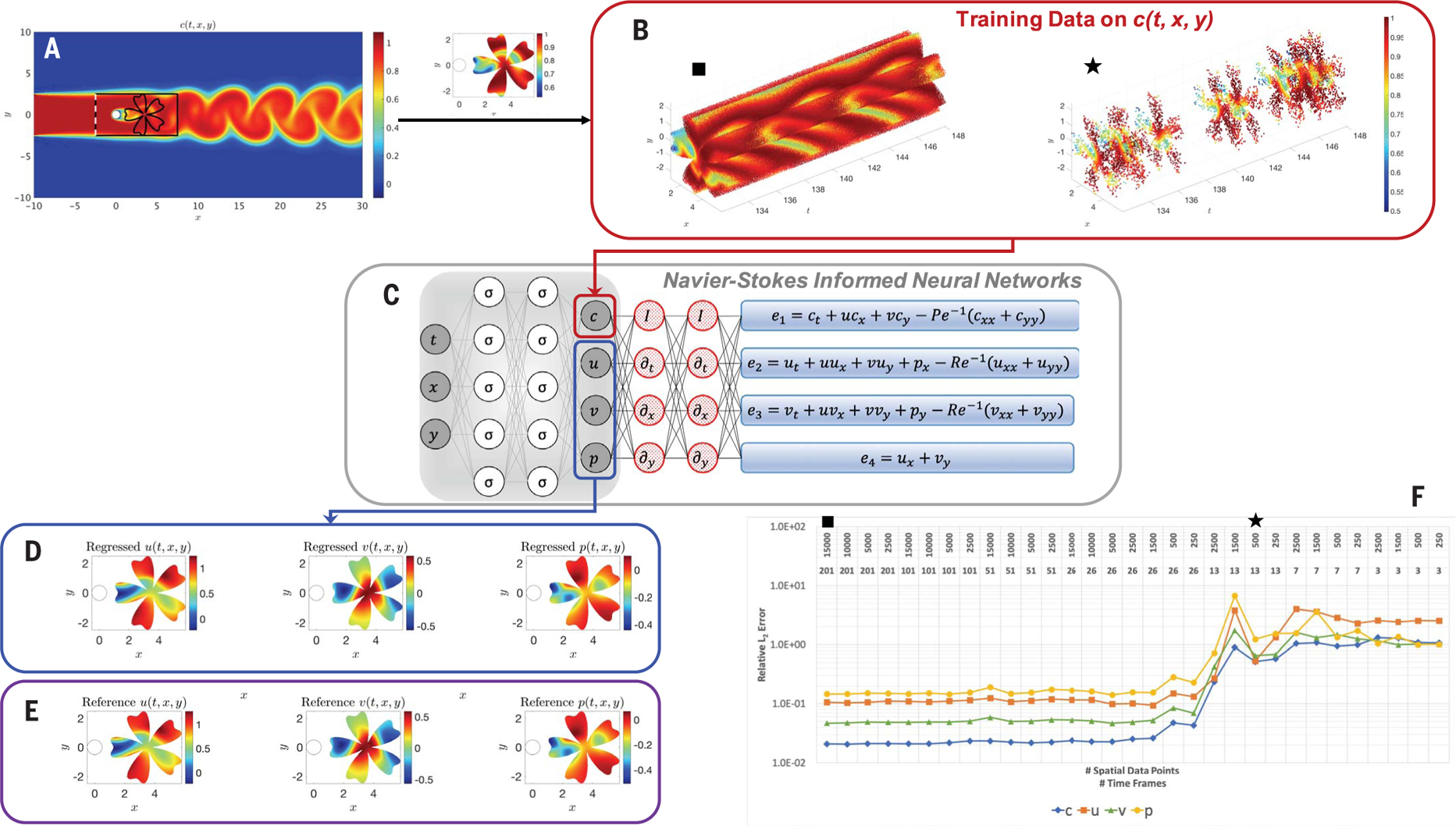
Fig. 2. Arbitrary training domain in the wake of a cylinder.

(A) Domain where the training data for concentration and reference data for the velocity and pressure are generated by using direct numerical simulation. (B) Training data on concentration c(t, x, y) in an arbitrary domain in the shape of a flower located in the wake of the cylinder. The solid black square corresponds to a very refined point cloud of data, whereas the solid black star corresponds to a low-resolution point cloud. (C) A physics-uninformed neural network (left) takes the input variables t, x, and y and outputs c, u, v, and p. By applying automatic differentiation on the output variables, we encode the transport and NS equations in the physics-informed neural networks e_i, i = 1, …, 4 (right). (D) Velocity and pressure fields regressed by means of HFM. (E) Reference velocity and pressure fields obtained by cutting out the arbitrary domain in (A), used for testing the performance of HFM. (F) Relative L₂ errors estimated for various spatiotemporal resolutions of observations for c. On the top line, we list the spatial resolution for each case, and on the line below, we list the corresponding temporal resolution over 2.5 vortex shedding cycles.